Tabling and Answer Subsumption for Reasoning on Logic Programs with Annotated Disjunctions

TABLING AND ANSWER SUBSUMPTION FOR REASONING ON LOGIC PROGRAMS WITH ANNOTATED DISJUNCTIONS

FABRIZIO RIGUZZI1 AND TERRANCE SWIFT2

1 _{ENDIF – Universit`a di Ferrara, Via Saragat 1, Ferrara, Italy}

E-mail address: [email protected] 2

CENTRIA – Universidade Nova de Lisboa, Quinta da Torre 2829-516, Caparica, Portugal E-mail address: [email protected]

Abstract. The paper presents the algorithm “Probabilistic Inference with Tabling and

Answer subsumption” (PITA) for computing the probability of queries from Logic Pro-grams with Annotated Disjunctions. PITA is based on a program transformation tech-niques that adds an extra argument to every atom. PITA uses tabling for saving intermedi-ate results and answer subsumption for combining different answers for the same subgoal. PITA has been implemented in XSB and compared with the ProbLog,cplintand CVE systems. The results show that in almost all cases, PITA is able to solve larger problems and is faster than competing algorithms.

Introduction

Languages that are able to represent probabilistic information have a long tradition in Logic Programming, dating back to [Sha83, van86]. With these languages, it is pos-sible to model domains which contain uncertainty, situation often appearing in the real world. Recently, efficient systems have started to appear for performing reasoning with these languages [DR07, Kim08]

Logic Programs with Annotated Disjunction (LPADs) [Ven04] are a particularly inter-esting formalism because of the simplicity of their syntax and semantics, along with their ability to model causation [Ven09]. LPADs share with many other languages a distribu-tion semantics [Sat95]: a theory defines a probability distribudistribu-tion over logic programs and the probability of a query is given by the sum of the probabilities of the programs where the query is true. In LPADs the distribution over logic programs is defined by means of disjunctive clauses in which the atoms in the head are annotated with a probability.

Various approaches have appeared for performing inference on LPADs. [Rig07] proposed

cplint that first finds all the possible explanations for a query and then makes them mutually exclusive by using Binary Decision Diagrams (BDDs), similarly to what has been proposed for the ProbLog language [DR07]. [Rig08] presented SLGAD resolution that extends SLG resolution by repeatedly branching on disjunctive clauses. [Mee09] discusses the CVE algorithm that first transforms an LPAD into an equivalent Bayesian network and then performs inference on the network using the variable elimination algorithm.

Key words and phrases: Probabilistic Logic Programming, Tabling, Answer Subsumption, Logic Pro-grams with Annotated Disjunction, Program Transformation.

c

F. Riguzzi and T. Swift

CC

Creative Commons Non-Commercial No Derivatives License

Technical Communications of the 26th International Conference on Logic Programming, Edinburgh, July, 2010 Editors: Manuel Hermenegildo, Torsten Schaub

LIPIcs - Leibniz International Proceedings in Informatics. Schloss Dagstuhl - Leibniz-Zentrum für Informatik, Germany Digital Object Identifier: 10.4230/LIPIcs.ICLP.2010.162

In this paper, we present the algorithm “Probabilistic Inference with Tabling and An-swer subsumption” (PITA) for computing the probability of queries from LPADs. PITA builds explanations for every subgoal encountered during a derivation of the query. The explanations are compactly represented using BDDs that also allow an efficient computa-tion of the probability. Since all the explanacomputa-tions for a subgoal must be found, it is very useful to store such information so that it can be reused when the subgoal is encountered again. We thus propose to use tabling, which has recently been shown useful for probabilis-tic logic programming in [Kam00, Rig08, Kim09, Man09]. This is achieved by transforming the input LPAD into a normal logic program in which the subgoals have an extra argument storing a BDD that represents the explanations for its answers. Moreover, we also exploit answer subsumption to combine different explanations for the same answer. PITA is tested on a number of datasets and compared with cplint, CVE and ProbLog [Kim08]. The algorithm was able to successfully solve more complex queries than the other algorithms in most cases, and it was also almost always faster.

The paper is organized as follows. Section 1 briefly recalls tabling and answer subsump-tion. Section 2 illustrates syntax, semantics and inference for LPADs. Section 3 presents PITA, Section 4 describes the experiments and Section 5 concludes the paper.

1. Tabling and Answer Subsumption

The idea behind tabling is to maintain in a table both subgoals encountered in a query evaluation and answers to these subgoals. If a subgoal is encountered more than once, the evaluation reuses information from the table rather than re-performing resolution against program clauses. Although the idea is simple, it has important consequences. First, tabling ensures termination of programs with thebounded term size property. A program P has the bounded term size property if there is a finite functionf :N →N such that if a query term Q to P has size size(Q), then no term used in the derivation of Q has size greater than f(size(Q)). This makes it easier to reason about termination than in basic Prolog. Second, tabling can be used to evaluate programs with negation according to the Well-Founded Semantics (WFS) [van91]. Third, for queries to wide classes of programs, such as datalog programs with negation, tabling can achieve the optimal complexity for query evaluation. And finally, tabling integrates closely with Prolog, so that Prolog’s familiar programming environment can be used, and no other language is required to build complete systems. As a result, a number of Prologs now support tabling, including XSB, YAP, B-Prolog, ALS, and Ciao. In these systems, a predicate p/n is evaluated using SLDNF by default: the predicate is made to use tabling by a declaration such as table p/n that is added by the user or compiler.

This paper makes use of a tabling feature calledanswer subsumption. Most formulations of tabling add an answer A to a table for a subgoal S only if A is a not a variant (as a term) of any other answer for S. However, in many applications it may be useful to order answers according to a partial order or (upper semi-)lattice. In the case of a lattice, answer subsumption may be specified by means of a declaration such as table p( ,or/3 - zero/1)).

where a lattice is defined on the second argument by providing a bottom element (returned by zero/1) and a join operation (or/3). With the previous declaration, if a table contains an answerp(a, E1) and a new answer p(a, E2) were derived, the answer p(a, E1) is replaced

upper semi-lattices is implemented in XSB for stratified programs [Swi99]; in addition, the mode-directed tabling of B-Prolog can also be seen as a form of answer subsumption.

2. Logic Programs with Annotated Disjunctions

A Logic Program with Annotated Disjunctions [Ven04] consists of a finite set of anno-tated disjunctive clauses of the form h1 :α1 ; . . . ; hn:αn← b1, . . . , bm. In such a clause

h1, . . . hn are logical atoms andb1, . . . , bm are logical literals,{α1, . . . , αn}are real numbers

in the interval [0,1] such that Pn

j=1αj ≤ 1. h1 : α1 ; . . . ; hn : αn is called the head and b1, . . . , bm is called the body. Note that if n = 1 and α1 = 1 a clause corresponds to

a normal program clause, sometimes called a non-disjunctive clause. If Pn

j=1αj < 1, the

head of the annotated disjunctive clause implicitly contains an extra atom null that does not appear in the body of any clause and whose annotation is 1−Pn

j=1αj. For a clause C of the form above, we define head(C) as {(hi : αi)|1 ≤ i ≤ n} if Pn

i=1αi = 1 and as

{(hi :αi)|1≤ i≤ n} ∪ {(null : 1−

Pn

i=1αi)} otherwise. Moreover, we define body(C) as

{bi|1≤i≤m},hi(C) ashi and αi(C) as αi.

If LPAD T is ground, a clause represents a probabilistic choice between the non-disjunctive clauses obtained by selecting only one atom in the head. If T is not ground, it can be assigned a meaning by computing its grounding, ground(T). The semantics of LPADs, given in [Ven04], requires the ground program to be finite, so the program must not contain function symbols if it contains variables.

By choosing a head atom for each ground clause of an LPAD we get a normal logic pro-gram called apossible world of the LPAD (instance in [Ven04]). A probability distribution is defined over the space of possible worlds by assuming independence between the choices made for each clause.

More specifically, anatomic choice is a triple (C, θ, i) whereC ∈T,θis a substitution that grounds C and i∈ {1, . . . ,|head(C)|}. (C, θ, i) means that, for ground clauseCθ, the head hi(C) was chosen. A set of atomic choices κ is consistent if (C, θ, i) ∈ κ,(C, θ, j) ∈

κ ⇒ i = j, i.e., only one head is selected for a ground clause. A composite choice κ is a consistent set of atomic choices. TheprobabilityP(κ)of a composite choice κis the product of the probabilities of the individual atomic choices, i.e. P(κ) =Q

(C,θ,i)∈καi(C).

A selection σ is a composite choice that, for each clauseCθinground(T), contains an atomic choice (C, θ, i) in σ. We denote the set of all selections σ of a program T by ST. A selection σ identifies a normal logic program wσ defined as follows: wσ = {(hi(C) ← body(C))θ|(C, θ, i) ∈ σ}. wσ is called a possible world (or simply world) of T. Since selections are composite choices, we can assign a probability to possible worlds: P(wσ) = P(σ) =Q

(C,θ,i)∈σαi(C).

We consider only soundLPADs in which every possible world has a total well-founded model. In this way, the uncertainty is modeled only by means of the disjunctions in the head and not by the features of the semantics. In the following we write wσ |=φto mean that the closed formula φis true in the well-founded model of the program wσ.

The probability of a closed formula φaccording to an LPAD T is given by the sum of the probabilities of the possible worlds where the formula is true according to the WFS: P(φ) =P

σ∈ST,wσ|=φP(σ). It is easy to see that P satisfies the axioms of probability. Example 2.1. The following LPAD encodes the dependency of a person’s sneezing on his having the flu or hay fever:

ciao 3 2 1 a0a ciao ₁ 3 2 a1a XC1∅ XC2∅ (a) MDD. ciao 0 1 a0a ciao ₁ 0 a1a XC1∅1 XC2∅1 (b) BDD.

Figure 1: Decision diagrams for Example 2.1.

C1 = strong sneezing(X) : 0.3 ; moderate sneezing(X) : 0.5 ← f lu(X).

C2 = strong sneezing(X) : 0.2 ; moderate sneezing(X) : 0.6 ← hay f ever(X).

C3 = f lu(david).

C4 = hay f ever(david).

If the LPAD contains function symbols, its semantics can be given by following the approach proposed in [Poo00] for assigning a semantics to ICL programs with function symbols. A similar result can be obtained using the approach of [Sat95]. In a forthcoming extended version of this paper we discuss how this can be done.

In order to compute the probability of a query, we can first find acovering set of explana-tions and then compute the probability from them. A composite choiceκidentifies a set of possible worldsωκ that contains all the worlds relative to a selection that is a superset ofκ, i.e., ωκ={wσ|σ∈ ST, σ⊇κ}. Similarly we can define the set of possible worlds associated to a set of composite choicesK: ωK =

S

κ∈Kωκ. Given a closed formula φ, we define the notion of explanation and of covering set of composite choices. A finite composite choiceκis anexplanation forφifφis true in every world ofωκ. In Example 2.1, the composite choice

{(C1,{X/david},1)} is an explanation for strong sneezing(david). A set of choices K is

covering with respect toφif every worldwσ in whichφis true is such thatwσ ∈ωK. In Ex-ample 2.1, the set of composite choices L1 ={{(C1,{X/david},1)},{(C2,{X/david},1)}}

is covering forstrong sneezing(david). Moreover, both elements ofL1 are explanations, so

L1 is a covering set of explanations for the querystrong sneezing(david).

We associate to each ground clause Cθ appearing in a covering set of explanations a multivalued variable XCθ with values {1, . . . , head(C)}. Each atomic choice (C, θ, i) can then be represented by the propositional equation XCθ = i. If we conjoin equations for a single explanation and disjoin expressions for the different explanations we obtain a Boolean function that assumes value 1 if the values assumed by the multivalued variables correspond to an explanation for the goal. Thus, if K is a covering set of explanations for a query φ, the probability of the Boolean formula f(X) =W

κ∈K

V

(C,θ,i)∈κXCθ =i taking value 1 is

the probability of the query, where Xis the set of all ground clause variables.

For example, the covering set of explanations L1 translates into the function f(X) =

(XC1∅ = 1)∨(XC2∅ = 1). Computing the probability of f(X) taking value 1 is equivalent to computing the probability of a DNF formula which is an NP-hard problem. In order to solve it as efficiently as possible we use Decision Diagrams, as proposed by [DR07].

A Multivalued Decision Diagram (MDD) [Tha78] represents a function f(X) taking Boolean values on a set of multivalued variablesXby means of a rooted graph that has one level for each variable. Each node has one child for each possible value of the multivalued variable associated to the level of the node. The leaves store either 0 or 1. For example, the MDD corresponding to the function forL1 is shown in Figure 1(a). MDDs represent a

can be computed by means of a dynamic programming algorithm that traverses the MDD and sums up probabilities.

Decision diagrams can be built with various software packages that provide highly efficient implementation of Boolean operations. However, most packages are restricted to work on Binary Decision Diagram (BDD), i.e., decision diagrams where all the variables are Boolean [Bry86]. To work on MDD with a BDD package, we must represent multivalued variables by means of binary variables. Various options are possible, we found that the following, proposed in [DR08], gives the best performance. For a variable X having n values, we usen−1 Boolean variables X1, . . . , Xn−1 and we represent the equation X =i

fori= 1, . . . n−1 by means of the conjunctionX1∧X2∧. . .∧Xi−1∧Xi, and the equation

X = n by means of the conjunction X1∧X2 ∧. . .∧Xn−1. The BDD representation of

the function forL1 is given in Figure 1(b). The Boolean variables are associated with the

following parameters: P(X1) =P(X = 1), . . . , P(Xi) = Qi−P1(X=i) j=1(1−P(Xj))

.

3. Program Transformation

The first step of the PITA algorithm is to apply a program transformation to an LPAD to create a normal program that contains calls for manipulating BDDs. In our implemen-tation, these calls provide a Prolog interface to the CUDD1_{C library and use the following}

predicates2

• init, end: for the allocation and deallocation of a BDD manager, a data structure used to keep track of the memory for storing BDD nodes;

• zero(-BDD), one(-BDD), and(+BDD1, +BDD2, -BDDO), or(+BDD1, +BDD2,

-BDDO), not(+BDDI, -BDDO): Boolean operations between BDDs;

• add var(+N Val, +Probs, -Var): addition of a new multi-valued variable withN Val

values and parameters Probs;

• equality(+Var, +Value, -BDD):BDD representsVar=Value, i.e. that the variable

Var is assignedValue in the BDD;

• ret prob(+BDD, -P): returns the probability of the formula encoded by BDD.

add var(+N Val,+Probs,-Var) adds a new random variable associated to a new instantia-tion of a rule with N Val head atoms and parameters list Probs. The auxiliary predicate

get var n/4 is used to wrap add var/3 and avoid adding a new variable when one already exists for an instantiation. As shown below, a new factvar(R,S,Var) is asserted each time a new random variable is created, whereR is an identifier for the LPAD clause,S is a list of constants, one for each variable of the clause, and Var is an integer that identifies the random variable associated with clause R under groundingS. The auxiliary predicates has the following definition

get var n(R, S, P robs, V ar)←

(var(R, S, V ar)→true;

length(P robs, L), add var(L, P robs, V ar), assert(var(R, S, V ar))).

whereR,S and Probs are input arguments while Var is an output argument. The PITA transformation applies to clauses, literals and atoms.

• Ifh is an atom,P IT Ah(h) ishwith the variableBDD added as the last argument.

• If bj is an atom,P IT Ab(bj) isbj with the variable Bj added as the last argument.

1

http://vlsi.colorado.edu/~fabio/

In either case for an atoma,BDD(PITA(a)) is the value of the last argument ofP IT A(a),

• If bj is negative literal¬aj,P IT Ab(bj) is the conditional

(P IT A0_b(aj) → not(BNj, Bj);one(Bj)), where P IT A0_b(aj) is aj with the variable BNj added as the last argument.

In other words, the BDD BNj for a is negated if it exists (i.e. P IT A0_b(aj) succeeds); otherwise the BDD for the constant function 1 is returned.

A non-disjunctive factCr=h is transformed into the clause P IT A(Cr) =P IT Ah(h)←one(BDD).

A disjunctive fact Cr = h1 : α1 ; . . . ; hn : αn. where the parameters sum to 1, is

transformed into the set of clauses P IT A(Cr)

P IT A(Cr,1) =P IT Ah(h1)← get var n(r,[],[α1, . . . , αn], V ar), equality(V ar,1, BDD).

. . .

P IT A(Cr, n) =P IT Ah(hn)← get var n(r,[],[α1, . . . , αn], V ar),

equality(V ar, n, BDD).

In the case where the parameters do not sum to one, the clause is first transformed into h1 :α1 ; . . . ; hn :αn ; null : 1−

Pn

1αi. and then into the clauses above, where the list of parameters is [α1, . . . , αn,1−Pn1αi] but the (n+ 1)-th clause (the one for null) is not generated.

The definite clauseCr=h←b1, b2, . . . , bm. is transformed into the clause P IT A(Cr) =P IT Ah(h)← P IT Ab(b1), P IT Ab(b2), and(B1, B2, BB2), . . . ,

P IT Ab(bm), and(BBm−1, Bm, BDD). The disjunctive clause

Cr=h1:α1 ; . . . ; hn:αn←b1, b2, . . . , bm.

where the parameters sum to 1, is transformed into the set of clausesP IT A(Cr) P IT A(Cr,1) =P IT Ah(h1)← P IT Ab(b1), P IT Ab(b2), and(B1, B2, BB2), . . . ,

P IT Ab(bm), and(BBm−1, Bm, BBm), get var n(r, V C,[α1, . . . , αn], V ar),

equality(V ar,1, B), and(BBm, B, BDD). . . .

P IT A(Cr, n) =P IT Ah(hn)← P IT Ab(b1), P IT Ab(b2), and(B1, B2, BB2), . . . ,

P IT Ab(bm), and(BBm−1, Bm, BBm), get var n(r, V C,[α1, . . . , αn], V ar),

equality(V ar, n, B), and(BBm, B, BDD).

whereV C is a list containing each variable appearing inCr. If the parameters do not sum to 1, the same technique used for disjunctive facts can be applied.

Example 3.1. Clause C1 from the LPAD of Example 2.1 is translated into

strong sneezing(X, BDD) ←flu(X, B1), get var n(1,[X],[0.3,0.5,0.2], V ar),

equality(V ar,1, B), and(B1, B, BDD).

moderate sneezing(X, BDD) ←flu(X, B1), get var n(1,[X],[0.3,0.5,0.2], V ar),

equality(V ar,2, B), and(B1, B, BDD).

while clauseC3 is translated into

f lu(david, BDD) ←one(BDD).

solve(Goal, P) ←init, retractall(var( , , )),

add bdd arg(Goal, BDD, GoalBDD),

(call(GoalBDD)→ret prob(BDD, P) ; P = 0.0), end.

Moreover, various predicates of the LPAD should be declared as tabled. For a predicatep/n, the declaration istable p( 1,..., n,or/3-zero/1), which indicates that answer subsumption is used to form the disjunct of multiple explanations: At a minimum, the predicate of the goal should be tabled; as in normal programs, tabling may also be used for to ensure termination of recursive predicates, or to reduce the complexity of evaluations.

PITA is correct for range restricted, bounded term-size and fixed-order dynamically stratified LPADs. A formal presentation with all proofs and supporting definitions will be reported in a forthcoming extended version of this paper.

4. Experiments

PITA was tested on programs encoding biological networks from [DR07], a game of dice from [Ven04] and the four testbeds of [Mee09]. PITA was compared with the exact version of ProbLog [DR07] available in the git version of Yap as of 19/12/2009, with the version of cplint [Rig07] available in Yap 6.0 and with the version of CVE [Mee09] available in ACE-ilProlog 1.2.20. All experiments were performed on Linux machines with an Intel Core 2 Duo E6550 processor (2333 MHz) and 4 GB of RAM.

The biological network problems compute the probability of a path in a large graph in which the nodes encode biological entities and the links represents conceptual relations among them. Each programs in this dataset contains a deterministic definition of path plus a number of links represented by probabilistic facts. The programs have been sampled from a very large graph and contain 200, 400, . . ., 5000 edges. Sampling has been repeated ten times, so overall we have 10 series of programs of increasing size. In each test we queried the probability that the two genes HGNC 620 and HGNC 983 are related.

We used the definition of path of [Kim08] that performs loop checking explicitly by keeping the list of visited nodes:

path(X, Y) ← path(X, Y,[X], Z).

path(X, Y, V,[Y|V]) ← edge(X, Y).

path(X, Y, V0, V1) ← edge(X, Z), append(V0, S, V1),

¬member(Z, V0), path(Z, Y,[Z|V0], V1).

This definition gave better results than the one without explicit loop checking. We are currently investigating the reasons for this unexpected behavior.

We ran PITA, ProbLog andcplinton the graphs in sequence starting from the smallest

program and in each case we stopped after one day or at the first graph for which the program ended for lack of memory3_{. In PITA, we used the group sift method for automatic}

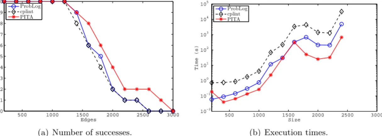
reordering of BDDs variables4. Figure 2(a) shows the number of subgraphs for which each algorithm was able to answer the query as a function of the size of the subgraphs, while Figure 2(b) shows the execution time averaged over all and only the subgraphs for which all the algorithms succeeded. PITA was able to solve more subgraphs and in a shorter time

3_{CVE was not applied to this dataset because the current version can not handle graph cycles.}

4_{For each experiment, we used either group sift automatic reordering or no reordering of BDDs variables} depending on which gave the best results.

500 1000 1500 2000 2500 3000 0 1 2 3 4 5 6 7 8 9 10 Edges Graphs ProbLog cplint PITA

(a) Number of successes.

500 1000 1500 2000 2500 3000 10−2 10−1 100 101 102 103 104 105 Size Time (s) ProbLog cplint PITA (b) Execution times.

Figure 2: Biological graph experiments.

0 20 40 60 80 100 0 0.2 0.4 0.6 0.8 1 N Time (s) cplint CVE PITA

Figure 3: Three sided die.

thancplintand ProbLog. For PITA the vast majority of time for larger graphs was spent on BDD maintenance.

The second problem models a game in which a die with three faces is repeatedly thrown until a 3 is obtained. This problem is encoded by the program

on(0,1) : 1/3 ; on(0,2) : 1/3 ; on(0,3) : 1/3. on(N,1) : 1/3 ; on(N,2) : 1/3 ; on(N,3) : 1/3←

N1 isN−1, N1≥0, on(N1, F),¬on(N1,3).

Form the above program, we query the probability of on(N,1) for increasing values of N. Note that this problem can also be seen as computing the probability that a Hidden Markov Model (HMM) is in state 1 at time N, where the HMM has three states of which 3 is an end state.

In PITA, we disabled automatic variable reordering. The execution times of PITA, CVE and cplint are shown in Figure 3. In this problem, tabling provides an impressive speedup, since computations can be reused often.

The four datasets of [Mee09], containing programs of increasing size. served as a final suite of benchmarks. bloodtype encodes genetic inheritance of blood type, growingbody

andgrowingheadcontains programs with growing bodies and heads respectively, anduwcse

20 40 60 80 10−3 10−2 10−1 100 101 102

Number of persons in family

Time (s) cplint CVE PITA (a)bloodtype. 5 10 15 20 25 30 35 40 10−3 10−2 10−1 100 N Time (s) cplint CVE PITA (b) growingbody.

Figure 4: Datasets from [Mee09].

5 10 15 20 10−4 10−2 100 102 104 106 N Time (s) cplint CVE PITA (a)growinghead. 0 5 10 15 10−4 10−2 100 102 104 Number of PhD students Time (s) cplint CVE PITA (b) uwcse.

Figure 5: Datasets from [Mee09].

for all datasets except foruwcse where we used group sift. The execution times of cplint, CVE and PITA are shown respectively in Figures 4(a), 4(b), 5(a) and 5(b)5_{. PITA was}

faster thancplintin all domains and faster than CVE in all domains exceptgrowingbody.

5. Conclusion and Future Works

This paper presents the algorithm PITA for computing the probability of queries from an LPAD. PITA is based on a program transformation approach in which LPAD disjunctive clauses are translated into normal program clauses.

The experiments substantiate the PITA approach which uses BDDs together with tabling with answer subsumption. PITA outperformed cplint, CVE and ProbLog in scal-ability or speed in almost all domains considered.

5_{For the missing points at the beginning of the lines a time smaller than 10}−6 _{was recorded. For the}

References

[Bry86] R. E. Bryant. Graph-based algorithms for boolean function manipulation.IEEE Trans. on Comput., 35(8):677–691, 1986.

[DR07] L. De Raedt, A. Kimmig, and H. Toivonen. ProbLog: A probabilistic Prolog and its application in link discovery. InInternational Joint Conference on Artificial Intelligence, pp. 2462–2467. 2007. [DR08] L. De Raedt, B. Demoen, D. Fierens, B. Gutmann, G. Janssens, A. Kimmig, N. Landwehr, T.

Man-tadelis, W. Meert, R. Rocha, V. Santos Costa, I. Thon, and J. Vennekens. Towards digesting the alphabet-soup of statistical relational learning. InNIPS*2008 Workshop on Probabilistic Program-ming. 2008.

[Kam00] Y. Kameya and T. Sato. Efficient EM learning with tabulation for parameterized logic programs. InComputational Logic,LNCS, vol. 1861, pp. 269–284. Springer, 2000.

[Kim08] A. Kimmig, V. Santos Costa, R. Rocha, B. Demoen, and L. De Raedt. On the efficient execution of ProbLog programs. In International Conference on Logic Programming, LNCS, vol. 5366, pp. 175–189. Springer, 2008.

[Kim09] A. Kimmig, B. Gutmann, and V. Santos Costa. Trading memory for answers: Towards tabling ProbLog. InInternational Workshop on Statistical Relational Learning. KU Leuven, Leuven, Bel-gium, 2009.

[Man09] T. Mantadelis and G. Janssens. Tabling relevant parts of SLD proofs for ground goals in a prob-abilistic setting. InColloquium on Implementation of Constraint and Logic Programming Systems. 2009.

[Mee09] W. Meert, J. Struyf, and H. Blockeel. CP-Logic theory inference with contextual variable elimination and comparison to BDD based inference methods. InInternational Conference on Inductive Logic Programming. KU LEuven, Leuven, Belgium, 2009.

[Poo00] D. Poole. Abducing through negation as failure: stable models within the independent choice logic. J. Log. Program., 44(1-3):5–35, 2000.

[Rig07] F. Riguzzi. A top down interpreter for LPAD and CP-logic. InCongress of the Italian Association for Artificial Intelligence,LNAI, vol. 4733, pp. 109–120. Springer, 2007.

[Rig08] F. Riguzzi. Inference with logic programs with annotated disjunctions under the well founded seman-tics. InInternational Conference on Logic Programming,LNCS, vol. 5366, pp. 667–771. Springer, 2008.

[Sat95] T. Sato. A statistical learning method for logic programs with distribution semantics. In Interna-tional Conference on Logic Programming, pp. 715–729. 1995.

[Sha83] E. Y. Shapiro. Logic programs with uncertainties: a tool for implementing rule-based systems. In International Joint conference on Artificial intelligence, pp. 529–532. Morgan Kaufmann Publishers Inc., 1983.

[Swi99] T. Swift. Tabling for non-monotonic programming.Ann. Math. Artif. Intell., 25(3-4):201–240, 1999. [Tha78] A. Thayse, M. Davio, and J. P. Deschamps. Optimization of multivalued decision algorithms. In

International Symposium on Multiple-Valued Logic, pp. 171–178. IEEE Computer Society Press, Los Alamitos, CA, USA, 1978.

[van86] M H van Emden. Quantitative deduction and its fixpoint theory. J. Log. Program., 30(1):37–53, 1986.

[van91] A. van Gelder, K.A. Ross, and J.S. Schlipf. Unfounded sets and well-founded semantics for general logic programs.J. ACM, 38(3):620–650, 1991.

[Ven04] J. Vennekens, S. Verbaeten, and M. Bruynooghe. Logic programs with annotated disjunctions. In International Conference on Logic Programming,LNCS, vol. 3131, pp. 195–209. Springer, 2004. [Ven09] J. Vennekens, M. Denecker, and M. Bruynooghe. CP-logic: A language of causal probabilistic events

and its relation to logic programming.Theory Pract. Log. Program., 9(3):245–308, 2009.

This work is licensed under the Creative Commons Attribution Non-Commercial No Deriva-tives License. To view a copy of this license, visithttp://creativecommons.org/licenses/ by-nc-nd/3.0/.