Experimental realization of an interferometric quantum circuit to increase the computational depth

(1)

DIPLOMARBEIT

Titel der Diplomarbeit

Experimental realization of an interferometric quantum

circuit to increase the computational depth

Verfasser

Yannick Ole Lipp

angestrebter akademischer Grad

Magister der Naturwissenschaften (Mag. rer.nat.)

Wien, 2011

Studienkennzahl lt. Studienblatt: A 411

Studienrichtung lt. Studienblatt: Diplomstudium Physik

(2)

(3)

Quantum computation

1.1 Introduction

When Richard Feynman first introduced the concept of a quantum computer [1] his motivation was a different one than what should lead to its popularization. He suggested that the difficult task of simulating generic quantum systems might be better suited to a machine operating on the quantum level itself, than it is to a classical computer. But with the beginning coherent control of quantum systems the focus had drifted to a different direction. A series of proof of principle imple-mentations of quantum algorithms that had been developed in the meantime was initiated [2, 3,4]. Their potential speedup over classical programs, albeit arguably of any practical value here, is most visible in Deutsch’s algorithm [5]. Public interest, however, is incited by the opportunities offered through Shor’s factoring algorithm [6], the Grover search algorithm [7] and more recently Lloyd’s algorithm for systems of linear equations [8].

Sensation has dulled a little as it became clear that practical implementations require resources beyond what quantum systems can offer presently. It is still unclear which system will provide the basis for future applications. Photons, for instance, struggle with the lack of strong nonlinearities that imposes the use of linear optics, but at the same time offer desirable features found in none of the competing quan-tum systems. Photonic qubits can be manipulated at room temperature, together with their speed and low decoherence, this makes them the obvious candidate for combining aspects of computation and communication. It should be considered that classical computers have found a variety of new applications with the advent of net-works, most prominently the Internet. Blind quantum computation [9], for instance, is a procedure that allows to securely, i.e. without revealing the content, perform a (quantum) computation on a remote server.

All quantum system are confronted with the urge of being scalable. KLM [10] have addressed this question with a proposal that shows a path to near-deterministic quantum circuits. Though several refinements [11,12,13] the resource requirements remain demanding. Most implementations of photonic circuits therefore rely on a

(6)

2 Chapter 1 : Quantum computation

clever use of interference and a measurement-induced nonlinearity. That is, to sift the observed detection events by some indication of success, e.g. a coincidence detection. Fast, efficient and photon-number resolving detectors are required to distinguish the individual outcomes. For miniaturization and to improve the interferometric stabil-ity, free-space optics experiments are replaced by chips with integrated waveguides [14,15,16].

Currently, the most pressing problem concerns the deterministic creation of single photons. The standard spontaneous parametric down-conversion source [17] impedes the transition from a handful to hundreds and more qubits due to their probabilistic nature and insufficient efficiency.

A new perspective is offered by the one-way computational scheme [18]. Until then quantum computation followed the methodology of the circuit model [19,20]. The quantum circuit model mimics a proven concept of classical computing. Any quantum algorithm– some unitary operation –is decomposed into a universal set of logic gates. In the one-way computational scheme an entangled state, typically a cluster state [21], serves as an initial resource. Being separated from the actual computation it may be created by probabilistic means without interrupting the pro-cess [22]. An algorithm is executed by performing a certain sequence of single-qubit measurements on the cluster qubits. The concept was readily adopted with photons [23]. The required error-correction, a consequence inseparably tied to the nonunitary evolution through measurements, was also demonstrated [24].

Recently, the view has shifted again [25] to Feynman’s original intent of using quantum computers to simulate physical systems. In [26] this idea has been con-cretized by showing how to approximately simulate the unitary evolution of a time-independent Hamiltonian with a quantum circuit. In particular the field of quantum chemistry has attended to this concept [27,28]. Later the repertoire was extended by a quantum version of the ubiquitous Metropolis algorithm that allows to simulate the equilibrium and static properties of quantum systems [29].

This work is intended to increase the computational depth of photonic quantum systems for both quantum computation and simulation by laying the basis for a universal two-qubit quantum computer.

1.2 Photonic qubits

The quantum analogue to a classical bit is a qubit [30], a two-level system that can live in any superposition of these discrete states. Single photons can serve as a physical body to a qubit. Both its internal (polarization, orbital angular momentum, etc.) and external (spacial path, arrival time, etc.) degrees of freedom can be utilized. It is also possible to use a combination of these which helps to increase the number of available qubits [31,32]. Most common are polarization encoding in which a hori-zontally polarized photon represents the logical value of 0 and a vertically polarized photon is a logical 1; and path encoding, where the presence of a single photon in one of two paths is mapped to a logical 0 and 1, respectively.

(7)

1.2. Photonic qubits 3

A single-qubit state has a graphical representation as a vector on the Bloch sphere (see Figure1.1).

Figure 1.1: Bloch sphere. Any pure single-qubit state can be written as a superposition of the computational basis states: |φi=η|Hi+ν|Vi, where the amplitudes, η and ν, are complex numbers restricted by the normalization constraint|η|2₊_|_ν_|2_{= 1}_{. A general density}

matrixρ=1₂(1+~b~σ)can be described by a Bloch vector~b, where~σis the vector of the Pauli matrices x,y and z. Pure states lie on the surface, while mixed states are situated in the body of the sphere.

(8)

(9)

Chapter 2

The quantum optics toolbox

This chapter briefly introduces the tools available to linear optics quantum compu-tation (LOQC) [33].

2.1 Single-photon source

The interaction of an electromagnetic field induces dipole moments in a dielectric medium. The macroscopic sum thereof is the polarizationP~. Expansion with respect to the fieldE~ yields [34]

P_i =χ(1)_ij E_j+χ(2)_ijkE_jE_k+χ(3)_ijklE_jE_kE_l+... , (2.1)

where the coupling to the field is described by χ(n) the n-th order susceptibility tensor andi, j, k, l={1,2,3}. In most materials the nonlinear χ(n>1) are small and the presence of a strong incident pump light field is necessary to observe higher-order effects. That way a medium with a nonvanishing χ(2)-term can show spontaneous parametric down-conversion (SPDC) [35]. A pump photon with energy, ¯hωp, and momentum,¯h~kp, spontaneously converts into two photons1 with energies, ¯hωs and

¯

hωi, and momenta, ¯h~ks and ¯h~ki. To see a significant contribution a phase matching condition

~_k_p₌~_k_s₊~_k_i _(2.2)

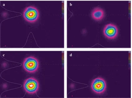
and energy conservationωp =ωs+ωi have to be satisfied simultaneously. This can be achieved by setting a specific angle between the pump beam and the orientation of the optical axis in the birefringent crystal [36]. With type-II phase matching [37] signal and idler photon are orthogonally polarized as defined by the orientation of the optical axis. Figure2.1 explains how to align a crystal such that ordinary and extraordinary axis correspond toH/V polarization, respectively. The correlation in the polarization degree of freedom can be used to generate entangled states [17]. For

1

They are historically referred to as signal and idler, as they always appear in pairs. The detection of the signal photon implies the presence of its partner, the idler.

(10)

6 Chapter 2 : The quantum optics toolbox

the purpose of quantum computation this feature is often unnecessary, but here the fact that pairs of photons are created in distinct time intervals is appreciated.

Figure 2.1: Aligning a nonlinear crystal to be used for SPDC. The crystal is mounted such that it can be rotated in the plain perpendicular to the incident, horizontally polarized light. (a) By convention H is supposed to travel along the ordinary axis. (b) Ordinary and extraordinary axis can be distinguished by rotating the mount. The intensity wanders between two spots. One remains at the same position (ordinary), while the other prescribes a circle around it (extraordinary). (c) Change to D-polarized light to place both spots above each other. (d) Send inV-polarized light to verify that it is aligned to the extraordinary axis.

The conversion process can occur at random along the length of the medium causing a horizontal walk-off effect. Likewise, the crystal’s birefringence is responsible for a transversal walk-off in the extraordinary beam. Both effects can be compensated by another nonlinear crystal with half the thickness [36,38].

To increase the probability for a coherent multi-pair emission the high energy density of pulsed lasers can be used. Coherence between the pairs is preserved when the pulse length that limits the temporal uncertainty associated with the creation time of the photon pairs is smaller than their coherence time. A shorter pulse duration, however, leads to a broader spectral bandwidth of the pump beam. As a consequence the overlap between energy conservation and the phase matching condition (2.2) increases and a larger range of frequencies is found in the down-converted beams. On the other hand, the coherence time can be extended by spectral filtering. Both the pulse length and the bandwidth of the filter should be adjusted to optimize the count rates. Due to an asymmetry in the phase matching function one of the down-converted spectra grows more quickly than the other [39]. Accordingly, filtering is asymmetric as the spectral bandwidth of ordinarily and extraordinarily polarized photons differ. Therefore an imbalance between H and V is observed.

(11)

2.2. Wave plates 7

For the experiments described in this work a femto-second pulsed laser at 789nm was frequency-doubled to pump a 2mm beta-barium borate (BBO) crystal in a non-colinear type-II configuration. In addition filters of 3nm bandwidth were used.

2.2 Wave plates

The polarization state of photons can be manipulated with wave plates. Commonly made of uniaxial birefringent crystals, they induce a relative phase shift between the (linear) polarization component aligned with the ordinary and the extraordinary axis [40]

∆ϕ= 2π

λ d(|no−ne|), (2.3)

where the thicknessdcan be set. Note that there is a dependence on the wavelength limiting the intended effect to a certain spectral range. Mostly, two kinds of wave plates are used: half-wave plates (_hwp) and quarter-wave plates (_qwp); introducing a phase shift of∆ϕ=π and ∆ϕ= π₂, respectively.

Rotating the wave plate in the plain perpendicular to the incident light corre-sponds to a change in basis and affects how the polarization amplitudes are split. The effect of _hwpand _qwpcan be written as unitary operators [41]

U_hwp(θ) =eiπ2 cos2θ sin2θ sin2θ −cos2θ , (2.4) U_qwp(θ) = √1 2 1 +i cos2θ i sin2θ i sin2θ 1−i cos2θ , (2.5)

where the angleθdenotes the orientation of the optical axis with respect to horizontal polarization. For some common angles the effect of _hwp and_qwpon the standard bases states is listed in TablesA.1andA.2 in the appendix.

Their property to alter the polarization state of a photon makes them suitable for implementing single-qubit unitaries. An arbitrary single-qubit unitary operation

U– a rotation on the Bloch sphere2 –can be decomposed into a combination of three wave plates [41]

U =U_qwp(γ)U_hwp(β)U_qwp(α). (2.6) To transform any polarization state to H or V, two wave plates, a _qwp and a hwp, are enough

U→H/V =Uhwp(β)Uqwp(α). (2.7)

The _qwp brings a potentially elliptical state to the x-z plane, where states with linear polarization are situated. For these states applying a _hwp corresponds to a

2

U =eiδR~b(ω), whereR~b(ω)is a rotation ofωabout the axis defined by the unit Bloch vector

~b. The global phaseeiδis usually ignored. The remaining three free parameters are set by the wave plate anglesα, βandγ.

(12)

rotation about the y axis and can thus map any such state to H/V. Table 2.1lists the required angles for some common polarizations.

Input → _qwp _hwp → Output

H/V 0◦ 0◦ H/V

D/A 45◦ 22.5◦ H/V

R/L 45◦ 45◦ H/V

Table 2.1: How to transform standard bases to the H/V basis using a _qwp and a _hwp. Note that _qwp and _hwp do not commute, so the angles are specific to the given order.

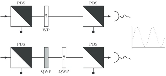
Before a wave plate can be used the position of the optical axis needs to be determined (Figure 2.2).

Figure 2.2: Aligning a wave plate. Place an unknown wave plate between two polarizing beam splitters and monitor the intensity, while rotating it in the plain perpendicular to the in-cident light. For some angle the intensity reaches a minimum: (_hwp) when the polarization is flipped fromH toV; (_qwp) the linear polarization is transformed to circular polarization. Refer to TablesA.1andA.2to determine the axis position from this information. Attention must be given that all _qwps are aligned to the same axis, ordinary or extraordinary. Use a reference _qwp: two _qwps aligned to the same axis will act as an effective _hwp, while compensating each other when not.

2.3 Beamsplitters

A beam splitter (BS) is a probabilistic device mediating between two spacial input and output modes. It is characterized by its transmission (reflection) probability T

(R). The most common configuration is a 50/50 beam splitter with T_R = 1.

Beam splitters can be designed to have different properties with respect to the polarization of the incident light, then called polarizing beam splitters (PBS). The

(13)

2.4. Mirrors, fibres and free space 9

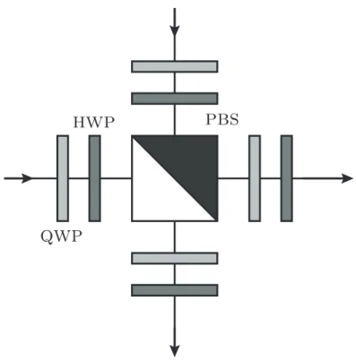
usual setting is that a PBS transmits H- and reflects V-polarized light. By sand-wiching a PBS between a set of wave plates it can be changed to operate in a basis other than the defaultH/V (Figure2.3a). Moreover, it can be used to translate from a polarization encoded qubit to a path encoded qubit and vice versa (Figure2.3b).

A subclass of polarizing beam splitters are polarization-dependent beam splitters (PDBS) that behave asymmetrically forH andV. PDBSs form a crucial component of the two-qubit gate presented in Chapter4. The variant to be used there, transmits allH-polarized light, while aV-polarized photon passes through in one third and is reflected in the remaining two thirds of the cases.

Occasionally, both input modes of a beam splitter are used to produce a Hong-Ou-Mandel two-photon interferometer type effect [42]. For a pair of photons, originating from a SPDC source, one is fed into the BS from either side. When the paths are shifted towards equal lengths, a decrease in the coincidence count rates is observed. The counts drop to a minimum when the difference is within the coherence length of the photons.

It is tempting to conclusively picture this as the result of interference between two individual photons indistinguishable at the BS. It was however clarified [43] that not the indistinguishability of the single photons at the BS, but of the two-photon amplitudes describing the various alternatives leading to a coincident count at the detectors is decisive. In the BS scenario four such alternatives exist: two cases where the photons exit at the same port, one transmitted one reflected (t-r & r-t), and two cases where they split up (r-r & t-t). When the paths are of exactly the same length, the cases t-t and r-r are indistinguishable and happen to interfere destructively in correspondence with the observed coincidence count rates.

A slightly modified experiment can rule out the single-photon interpretation (Fig-ure 2.4). A relative delay is introduced such that the photons no longer arrive at the same time at the beam splitter. This clearly eliminates the first interpreta-tion. But when the delay is compensated afterwards, producing the same relative time difference at the detectors for both alternatives, t-t and r-r, which makes them indistinguishable again, the dip in coincidence count rates returns.

2.4 Mirrors, fibres and free space

It is a common situation that two distinct parts of a setup need to be connected. Usually, the experimenter wants the state of the quantum system to remain the same before and after the passage. In contrast to other quantum systems photons are mostly unaffected by the environment. However, there are certain pitfalls to be avoided.

Frequently, light travels in free space. Dust particles floating in the air can cause deformations in the (Gaussian) beam profile of high-intensity laser beams. To recover a clean Gaussian shape the following procedure can be employed:

(14)

(a) Polarizing beam splitters are usually manufactured to operate on

H/V polarization. Using wave plates an arbitrary basis PBS can be emulated. Before the photons enter the PBS they pass through a hwp and qwpwith angles set such that they transform from the desired op-eration basis to theH/V basis. The procedure is reversed at the output ports of the PBS.

(b) Converting between polarization encoding and path encoding of a photonic qubit. A PBS separates H and V components into distinct paths faithful to their respective amplitudes. To make them indistin-guishable by the polarization degree of freedom ahwpat45◦transforms |Vi ↔ |Hi. Backtransformation is feasible by reversing the order of the components.

(15)

2.4. Mirrors, fibres and free space 11

Figure 2.4: Postponed compensation experiment [43]. One of two photons is delayed (in-dicated by the dashed line), so they no longer meet at the beam splitter. An additional delay for the t-t case assures that detectorD2 fires first in both situations. As the relative time

difference stays constant r-r and t-t become indistinguishable. Accordingly, the dip in the coincidence count rates is observed, despite the single-photon interference interpretation no longer applicable.

the beam and calculate the beam waist at the focal point.

2. The image at the focal point is the Fourier transform of the image at the object-side focal point [40]. Finer details, like deformations, require higher spatial frequencies to be resolved. The higher the frequency, the further off the corresponding amplitude lies from the centre of the Fourier image [44]. With a suitable iris the outer parts containing the frequency information of the deformations can be cut away.

3. Use another identical lens to undo the Fourier transform and collimate the beam again.

When the beam shape has become elliptical, e.g. after the up-conversion process in a LBO crystal [45], the sequence of two cylindrical lenses can be used to correct it back to a circular form. See [46] for instructions on how to select the ratio of their focal lengths.

To change the propagation direction of a laser beam mirrors are used. It is impor-tant to respect the mirror’s angle of incident (AOI) specification. One discriminates between mirrors (AOI = 0◦) and turning mirrors (AOI = 45◦). When the polar-ization of photons is an issue a mirror is no longer a neutral element, but has the effect of a half-wave plate set to0◦, hence it flips D/A → A/D and R/L → L/R.

(16)

Whenever there is an unbalanced number of mirrors3in the setup this has to be com-pensated for, e.g. with a half-wave plate. Additionally, most mirrors have different reflection coefficients for H- andV-polarized light. This means that the amplitudes are treated unequally and a drift in the polarization is observed.

When light is coupled into an optical fibre, again its polarization state needs to be controlled. In an ideal fibre each polarization mode would propagate with identical velocity. Slight asymmetries in the fibre core cross-section and external stresses applied on the fibre such as bending alter the refractive index along the fibre. Differing velocities between the polarization modes in the fibre introduce a relative phase shift between them. This leads to a change in polarization.

The stress-induced birefringence of the fibre can also be used to compensate for these effects. In most cases the intermediate polarization state of the light in the fibre is unimportant as long as there is no effective change in the output state. Fibre polarization controllers (FPC) are used to intentionally apply stress on the fibre. To perform an arbitrary single-qubit operation the usual _qwp-_hwp-_qwp combination of a free-space setting is replaced by three fibre coils inlaid in the FPC paddles. Coiling the fibre induces stress, producing birefringence inversely proportional to the square of the coils’ diameters [47]. The number of turns specifies the wave plate’s type. One turn corresponds to a_qwp, two to a_hwp. Adjusting the paddles rotates the fast axis of the fibre, which lies in the plane specified by the paddle.

To build a polarization conserving fibre path it is necessary to pinpoint both angles,θ andϕ, that define a single-qubit state with respect to the Bloch sphere. A common choice is to fix|Hi and |Di. Obviously, one cannot align them simultane-ously, so the procedure has to be carried out iteratively in general. Note that fixing the orthogonal states |Hi and |Vi is not sufficient, as this imposes no constraint on the azimuthal angleϕ.

2.5 Single-photon detection

An important part in linear optics quantum computation falls to the detection sys-tem, as most implementations rely on a measurement-induced nonlinearity through postselection. What are the properties of a good detector?

• Capability to detect single photons

• High detection efficiency

• Low dark count rates

• Fast recovery time

• Photon-number resolving

(17)

2.5. Single-photon detection 13

The experiments presented here use avalanche photodiodes (APD) that are fast and can resolve single photons, but cannot distinguish between one and many and have a rather low detection efficiency of about 40%. This is a serious downside as it further lowers the observed count rates, especially since one is usually interested in coincidence detections4. For a twofold-coincidence the detection probability degrades already to about 16% with these detectors. Many new developments in this field offer considerable improvements. An overview of current single-photon detection architectures is found in [48].

In general detectors do not distinguish between photons of different polarizations. This is, however, a common requirement in many applications, e.g. quantum state tomography (see Section4.4.1). Figure2.5describes how to experimentally measure the polarization state of a photon in an arbitrary basis using wave plates, polarizing beam splitters and single photon detectors.

Figure 2.5: Polarization analysis of light in an arbitrary basis follows a general procedure: The state of the incoming photon is considered to be decomposed with respect to the desired measurement basis. The basis vectors of this basis are then mapped to theH/V basis (vectors) by applying a_qwp and a _hwpwith specific angle settings,αandβ (cf. (2.7)). Next a PBS is used to separateH- andV-polarization. Finally, each output is fed into a single photon detector. A click at the detector for horizontally polarized photons reveals the photon to have carried the polarization determined by the chosen map. To measure in theD/A basis, for example, the map (wave plate setting) needs to transform|Di → |Hiand|Ai → |Vi. When the detector for|Hiis triggered, one can deduce that the photon carried polarization|Di.

4_{A coincidence is the simultaneous detection of single photons at different detectors. To achieve}

nonzero count rates, a time window shorter than the gap between two successive pulses from the source is defined to characterizesimultaneous events.

(18)

(19)

Chapter 3

Arbitrary single-qubit unitaries

with wave plates

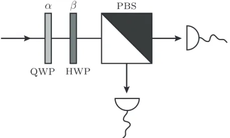
With photons single-qubit unitaries are generally considered the easy part. The main challenges come with the implementation of two-qubit gates (see Section 4). In principle this is true; applying single-qubit gates is a solved problem and can be accomplished by the use birefringent elements; typically wave plates. A few common single-qubit gates, along with the corresponding wave plate setting for their implementation, are listed in Table3.1.

Single-qubit gate Symbol Wave plate setting

Identity 1 _qwp(0)·_hwp(0)·_qwp(0) Pauli-X _x _hwp(π₄) Pauli-Y _y _hwp(π₄)·_hwp(0) Pauli-Z _z _hwp(0) Hadamard _h _hwp(π₈) X-rotation Rx(θ) qwp(π2)·hwp(− θ 4)·qwp( π 2) Y-rotation Ry(θ) qwp(π2 + θ 2)·hwp( θ 4)·qwp( π 2) Z-rotation Rz(θ) qwp(π₄)·hwp(−π₄ −θ₄)·qwp(π₄)

Table 3.1: Single-qubit gates and how to experimentally realize them using wave plates. Note that any gate may also introduce a global phase. The angleθ specifies the rotation as observed on the Bloch sphere, while the arguments of _hwpand _qwpare the corresponding physical angle settings of the wave plates.

There is, however, an easily overlooked aspect that needs to be considered. The operation of half and quarter-wave plate do not translate directly into rotations on the Bloch sphere. For general unitaries and with the interest of keeping the number of wave plates small1 this property becomes manifest. For each particular single-qubit

1

It would be possible to use the known patterns of Rx(θ), Ry(θ) and Rz(θ) to apply some

arbitrary rotation, but this would lead to an inefficient use of wave plates.

(20)

16 Chapter 3 : Arbitrary single-qubit unitaries with wave plates

gate the angle settings of the wave plates need to be determined.

3.1 Implementation with wave plates

Scenario I: One-way computational model

In the one-way computational model [18] an algorithm is defined by the shape of the entangled resource– a cluster state [21] –and a specific pattern of single-qubit measurements in directions along the x-y plane of the Bloch sphere. This includes, apart from the standard D/A and R/L, all states in between: |±ϕi = √1

2(|Hi ± eiϕ|Vi). In view of the polarization analysis setup described in Figure 2.5 a _hwp and a_qwpare needed

hwp(β)qwp(α) |±ϕi −→ |Hi/|Vi. (3.1) To successfully perform this transformation we need the angles αandβ. This is not as simple a task as it might seem at first sight. The wave plates perform nontrivial operations on the Bloch sphere. They introduce a global phase, which might have no effect in the experiment, but complicates the computational task of finding the correct angles. Additionally, the elements of the unitary matrices corresponding to the wave plates (cf. (2.4) and (2.5)) are trigonometric functions and thus α and

β are given only implicitly. Nonetheless, it appears there is a simple relation for determining the angles in this case

α= π 4 , (3.2) β = π 8 + ϕ 4 . (3.3)

Scenario II: Arbitrary measurement basis

Measuring in the x-y plane is only a subproblem of the more general problem to perform measurements in an arbitrary basis. Again, we have to determine the angles for the wave plates. Rewriting the problem in matrix form

hwp(β)qwp(α) s0₁ s0₂ ≡ s1 s2 =|si −→ 1 0 =|Hi or 0 1 =|Vi (3.4) provides a helpful insight. One component of the column vector representation of both |Hi and |Vi is zero. If we manage to find a transformation such that one component of |si is zero or at least smaller than a given threshold, we have found a solution regardless of the global phase factor. A simple numerical implementation of this strategy delivers correct results [49].

After a series of manipulations we also arrive at an analytical formula

α= arctan tanθ cosϕ 2 , (3.5) β = 1 2

arctan cosθ sin 2α cos 2α+ sinθ(cosϕ(sin 2α)2+ sinϕcos 2α

(21)

3.1. Implementation with wave plates 17

with Bloch sphere anglesθ andϕdefined by

~

s0(θ, ϕ) = cosθ

2 |Hi+e

iϕ_sinθ

2 |Vi . (3.7)

Scenario III: Arbitrary to arbitrary single-qubit transformation

Apparently, the numerical procedure of Scenario II works only on the special cases–

|Hi or |Vi –where the target state vector |ti has one zero component. What about transformations from some arbitrary to another arbitrary single-qubit state? From (2.6) we know that three wave plates should suffice

qwp(γ)hwp(β)qwp(α) s0₁ s0₂ ≡ s1 s2 =|si −→ t1 t2 =|ti . (3.8) Let us try to adopt the previous numerical approach to this problem. When the corresponding components, s1 =t1 and s2 =t2, are the equal,|si and |ti represent

the same state. Minimizing the sum of the absolute values of the differences

min

α,β,γ |s1−t1|+|s2−t2| (3.9) would give a valid solution. But the potential global phase factor complicates the situation. Suppose that |ti = |Di = √1

2 1 1

; a set of angles {α, β, γ}, producing

|si= √1

2 i i

is a correct solution. However, the minimization (3.9) returns

i √ 2 − 1 √ 2 + i √ 2− 1 √ 2 = 2. (3.10)

This solution is likely to be missed as many wrong angles lead to smaller values. To ensure a trustworthy result one would require (3.9) to be less than some threshold, certainly smaller than 2.

The problem is obviously due to a different global phase in|si and |ti. To cope with it we must bring them into a standardized form. One component of |si can always be made a real number by multiplying it with κ = e−arg(s1)_{. This has the}

effect of setting a default phase factor of +1. Without loss of generality we can assume|ti also to have this form, as it is chosen by the experimenter. The adapted method

min

α,β,γ |κs1−t1|+|κs2−t2| (3.11) returns valid solutions for all but a single case. When|ti=|Vi, the described phase problem persists2. Fortunately, this issue is easy to resolve, as we can fall back to the solution of scenario II whenever this happens.

2

Fors1= 0the introduced global phase is hidden andκis unable to bring|s0ito the standard

(22)

18 Chapter 3 : Arbitrary single-qubit unitaries with wave plates

The closed-form solution we found for measuring in an arbitrary basis suggests that one can also find a solution for this problem. From (3.6) we know how to use a qwpto transform a general state to a linear-polarization state. When we apply this technique from both ends,|s0iand|ti, we receive two states located in the x-z plane of the Bloch sphere. The intermediate_hwpcan map two such states onto each other. Appendix Bcontains aMathematica3 implementation of the outlined strategy.

3.2 A demonstration

We have acquired the means to perform any single-qubit transformation with just three wave plates. For each case, the initially unknown angles, α, β and γ, can be determined.

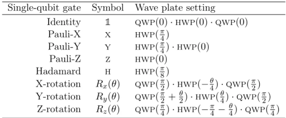
This calls for a demonstration. Consider two randomly chosen states

|s0i= 0.979 −0.142−0.148i α,β,γ −→ |ti= 0.892 0.404−0.202i ,

scattered around the Bloch sphere; see Figure 3.1aand 3.1d. We find

α= 90.8036, β = 18.2966 and γ = 18.8240.

It is instructive to visualize each step of the transformation individually. Figure 3.1

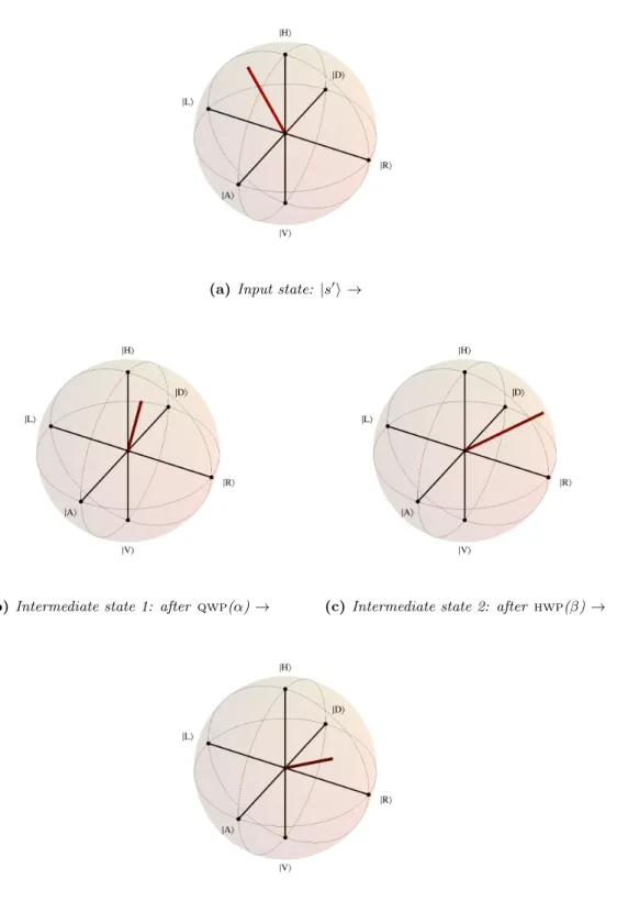
shows the intermediate Bloch vector after the application of each wave plate. To confirm the correctness of the angles, the experimentally obtained density matrices of the input state, |s0i, and the final state are compared in Figure 3.2

and3.3. Note the nonvanishing imaginary parts also in the theoretical values (cones). The state fidelities FS between experimental and theoretical data4

|s0i:FS = 99.3%,[98.8; 99.7] and |ti:FS = 99.6%,[98.0; 99.9] express a high level of agreement.

3

http://www.wolfram.com/mathematica/

4_{The fidelity is restricted to the interval} _{[0; 1]}_. _{Close to the boundaries its distribution is}

insufficiently described by a Gaussian fit. Instead, a bounded Johnson distribution [50] was used. A confidence interval containing approximately68%of the values is given in brackets.

(23)

3.2. A demonstration 19

(a) Input state: |s0i →

(b)Intermediate state 1: after qwp(α)→ (c) Intermediate state 2: after hwp(β)→

(d)Final state

Figure 3.1: The transformation process visualized on the Bloch sphere. For each step the resulting Bloch vector is shown.

(24)

20 Chapter 3 : Arbitrary single-qubit unitaries with wave plates ÈH\XHÈ ÈH\XVÈ ÈV\XHÈ ÈV\XVÈ 0.0 0.5

(a)Input state density matrix - Real

ÈH\XHÈ ÈH\XVÈ ÈV\XHÈ ÈV\XVÈ -0.1 0.0 0.1

(b) Input state density matrix - Imaginary

(25)

3.2. A demonstration 21 ÈH\XHÈ ÈH\XVÈ ÈV\XHÈ ÈV\XVÈ 0.0 0.2 0.4 0.6 0.8

(a)Final state density matrix - Real

ÈH\XHÈ ÈH\XVÈ ÈV\XHÈ ÈV\XVÈ -0.1 0.0 0.1 0.2

(b) Final state density matrix - Imaginary

Figure 3.3: Theoretical (cones) and experimental (bars) density matrices of the state after applyingUqhq =qwp(γ)hwp(β)qwp(α)to|s0i. The anglesα,β andγwere determined by

(26)

(27)

Chapter 4

Experimental realization of a

Controlled-

_not

gate

Inspired by its classical counterpart a circuit model for quantum computation was developed [19,20]. In this scheme an algorithm is implemented via unitary transfor-mation of a quantum state representing the input register. In analogy to a classical computer– e.g. _nand –a set of operations (gates) is sufficient to construct a uni-versal quantum computer capable of implementing generic quantum algorithms. As explained in more detail in [51] the set of all single-qubit unitaries together with a two-qubit gate1– e.g. _cnot –is universal for quantum computation. In brief; a quantum process on an input register of N qubits may be decomposed into smaller entities, because the corresponding multi-qubit unitary can be written as a product of operators that each act non-trivially only on a two-dimensional subspace. Single-qubit and _cnot gates, on the other hand, suffice to implement any such two-level unitary operation.

4.1 Properties of the

_cnot

gate

A controlled two-qubit operation assigns different roles to either qubit. One qubit (usually the first) is referred to as control qubit. Its state– a superposition of

|Hi : |0i : _false and |Vi : |1i : _true–controls the operation applied to the other

qubit, the target qubit. Apart from the already mentioned cnot, we look at an-other controlled gate called2 _csign. Their operation can be written as4×4unitary matrices

1

Single qubit unitaries alone are not enough because some sort of interaction is needed to create entanglement between qubits. Interestingly the mere presence of entanglement is not enough to gain the exponential speedup of some quantum algorithms either. As can be inferred from the Gottesman-Knill theorem [52] it is necessary to include gates outside the Clifford group for an algorithm not to be efficiently simulable on a classical computer, i.e. in the stabilizer formalism [53].

2_sometimes

cphase

(28)

24 Chapter 4 : Experimental realization of a Controlled-_not gate csign=     1 0 0 0 0 1 0 0 0 0 1 0 0 0 0 −1     (4.1) cnot=     1 0 0 0 0 1 0 0 0 0 0 1 0 0 1 0     (4.2)

or visualized in BraKet notation:

The _csign gate inflicts a sign flip on the amplitude cV V and acts as an identity

operation on the other components.

A different naming convention refers to _csign and _cnot by _cz and _cx, re-spectively, as they apply controlled Pauli _z and _x operations on the target qubit. This almost immediately lets us understand the identity relation established by local Hadamard gates3

where the symbol on the left hand side corresponds to a _cnot in the circuit repre-sentation.

With photons any experimental implementation of one of them, is equally suitable to obtain the other. Transformation is a simple matter of adding a pair of wave plates.

4.1.1 Implementation scheme

A compact scheme for a _csign gate has been formulated in [54, 55, 56]. Sec-tion 5.2compares several existing architectures and explains the advantages of this choice. The working principle of the gate unfolds by looking at the properties of a

3_{The Hadamard gate}

h=√1

(29)

4.1. Properties of the_cnotgate 25

Figure 4.1: Basic idea for the implementation of a _csign gate. Two photons entering a PDBS can exhibit four possible exit configurations. Postselecting for coincidence detections from both arms hides the spurious r-t and t-r cases. Below each scenario the possible coin-cidences are listed. As reflected photons pick up a phase factor, theV V term from r-r and t-t have opposite signs.

polarization-dependent beam splitter (Figure 4.1). When a pair of photons, one at each input port, is subjected to a PDBS four possible scenarios occur:

r-t : The first photon is reflected and the second is transmitted.

t-r : The first photon is transmitted and the second is reflected.

r-r : Both photons are reflected.

t-t : Both photons are transmitted.

A few important observations can be made. Firstly, the cases r-t and t-r lead to a different detection pattern than r-r and t-t. Assuming that both output ports are fed into separate detectors, the former cases will never trigger a simultaneous detection as both photons exit through the same output port. For the latter, the situation is reversed, it will always lead to a coincident detection.

Secondly, due to the asymmetric behaviour of a PDBS–H-polarized photons are transmitted, whileV-polarized photons have a certain chance of being reflected –the r-r case can only occur when both photons have a nonzeroV-polarization amplitude. Additionally, the reflected photons pick up a phase shift. This selectively applies a minus sign to the|V Viterm of the corresponding two-photon state, as it is expected from a_csigngate.

A V V coincidence without the phase change can, however, also happen in the course of a t-t event. When both cases– r-r and t-t –interfere the effective amplitude can be tuned by setting the V-polarization transmission probability of the (main) PDBS. The r-t and t-r events do not contribute to coincidence detections.

Another aspect that we will have to consider is that due to the interference the amplitudes of|HHi,|HVi,|V Hiand|V Viare different. To faithfully implement a

(30)

26 Chapter 4 : Experimental realization of a Controlled-_not gate

that can selectively attenuate the amplitudes. This can be done by another two (attenuation) PDBS placed in each arm of the setup.

4.1.2 Optimal components

and 2, a first PDBS (main) has the following effect

|H1i −→ τH|H1i + i κH|H2i |H2i −→ τH|H2i + i κH|H1i |V1i −→ τV |V1i + i κV |V2i |V2i −→ τV |V2i + i κV |V1i τX ≡ p TX, κX ≡ p RX with X={H, V}

whereTX/RXis the corresponding transmission/reflection probability forX-polarized light. Characteristic to a measurement-induced nonlinearity is that we choose to only look at coincidence detections, i.e. when there is a simultaneous click at both the control and the target arm4. With any term containing two identical indices already sifted out, the calculation yields5

|ψ0i= (cHHτHτH−cHHκHκH) |H1H2i

+(cHV τHτV −cV HκHκV) |H1V2i

+(cV HτHτV −cHV κHκV) |V1H2i

+(cV V τVτV −cV V κVκV) |V1V2i (4.5) This is of course only possible as soon as no further element in the setup can transfer a photon from one arm to the other.

Each arm is then subjected to another PDBS (attenuator), of which the reflected port is committed to a beam dump. Whenever one photon on either side suffers this fate no coincidence can occur and the corresponding terms can be left out. In general the transmission/reflection amplitudes of these PDBS can be different from the first, hence we prime them

|ψ00i= (cHHτHτHτH0 τ 0 H −cHHκHκHτH0 τ 0 H) |H1H2i +(cHV τHτVτH0 τ 0 V −cV HκHκVτH0 τ 0 V) |H1V2i +(cV HτHτVτH0 τV0 −cHV κHκVτH0 τV0 ) |V1H2i +(cV V τVτVτV0 τV0 −cV V κVκVτV0 τV0 ) |V1V2i. (4.6) 4_{When a polarization-aware detector setting (cf. Figure}_2.5_{) is used, this corresponds to the}

situation when one and only one detector of each arm is firing.

(31)

4.1. Properties of the_cnotgate 27

As can be seen from (4.3) a_csignscales (the modulus of) all amplitudes equally for anycHH, cHV, cV H andcV V. The only nontrivial solutions require eitherκV = 0or κH = 0. Choosing the latter the transmission/reflection amplitudes must fulfil the following condition τHτHτH0 τH0 ! =τHτVτH0 τV0 ! =−(τVτVτV0 τV0 −κVκVτV0 τV0 ) (4.7) apart from the restrictions due to the transmission/reflection probabilities: 0 < TX, RX ≤ 1 and TX +RX ≤ 1. Note the additional minus sign in front of the last term forming the _csign operation. κH = 0 already implies τH = 1, leaving

0< τ_H0 ≤ √1 3,τV = 1 √ 3 and τ 0 V = √ 3τ_H0 .

What value should we choose for τ_H0 ? To answer this question we must first determine what an optimal value should do. Scaling the amplitudes in (4.3) by a constant factorf means that only a fraction of the photons is observed at the control and target outputs. This reduces the probability of a successful gate operation by the square of that factor

ρ csign−→ (f×_csign)ρ(f ×_csign)†=f2×(csignρcsign†), (4.8) where ρ is the density matrix of some two-qubit state. The optimal value would therefore bef = 1. From (4.7) we see thatf(τ_H0 ) =τ_H02, thereforeτ_H0 = √1

3 ⇒f = 1 3

is our best option. Accordingly, the setup is expected to apply a successful _csgin operation in one ninth of the cases (= 11.¯1%).

This is another consequence of the measurement-induced nonlinearity scheme. In most cases the desired operation can only be realized with a certain chance; the gate becomes probabilistic. Fortunately, there is a clear distinction between correct and incorrect runs. A successful gate operation is unambiguously indicated by a coincidence detection.

In Table4.1the transmission and reflection probabilities corresponding tof = 1₃ are given, |ψ00i_f₌1 3 = 1 3 |H1H2i+ 1 3 |H1V2i+ 1 3 |V1H2i − 1 3 |V1V2i. (4.9) 4.1.3 Modelling imperfect components

Now that we know what properties ideal components should have, it is advisable to study the impact of deviations from these values on the gate. Let us therefore review the gate’s performance under the influence of imperfect components.

Considering the transmission probabilityTV of the main PDBS as a free param-eter affects the operation of_csignon an arbitrary input stateρin the following way (cf. (4.6))

(32)

28 Chapter 4 : Experimental realization of a Controlled-_not gate Main PDBS: TH = 100% TV = 33.˙3% RH = 0% RV = 66.˙6% Attenuation PDBS: T_H0 = 33.˙3% T_V0 = 100% R0_H = 66.˙6% R_V0 = 0%

Table 4.1: Optimal values of transmission and reflection probabilities for the PDBS to be used in the _csignsetup.

ρ −→ W ρ W†, where W(TV) =       1 3 0 0 0 0 q TV 3 0 0 0 0 q TV 3 0 0 0 0 2TV −1       . (4.10)

This model is equally valid for a_cnotgate implemented by(1⊗H)·_csign·(1⊗H), where the single-qubit Hadamard is assumed to be perfect.

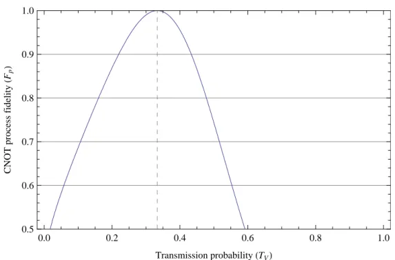
The process fidelity Fp is a suitable benchmark parameter6 to quantify the per-formance of a gate. In Figure 4.2 its dependence on the transmission probability of the main PDBS is shown. The simulation verifies the ideal value of TV = 1₃ we derived earlier. Apart from that it prognoses a moderate degradation when the ratio deviates from that value.

Similar considerations can be given to the influence of the attenuating PDBS. Here the roles ofH- andV-polarized light are interchanged. The effect of a variable

(33)

4.1. Properties of the_cnotgate 29 0.0 0.2 0.4 0.6 0.8 1.0 0.5 0.6 0.7 0.8 0.9 1.0 Transmission probabilityHTVL CNOT process fidelity H Fp L

Figure 4.2: Simulating the _cnotprocess fidelity for a varying transmission probabilityTV

of the main PDBS.

transmission probabilityT_H0 is modelled by

ρ −→ W0ρ W0†, where W0(T_H0 ) =       T_H0 0 0 0 0 q T0 H 3 0 0 0 0 q T_H0 3 0 0 0 0 −1₃       . (4.11)

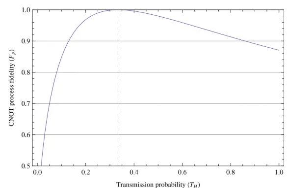
The required precision of these components are less demanding (see Figure4.3). In particular a transmission probability greater than 1₃ only gradually lowers the gate’s performance.

In Figure4.4imperfect transmission probabilities for either PDBS are considered (axes). A lighter shading corresponds to a higher_cnotprocess fidelity. The contour lines represent a lower bound forFp inside the enclosed region.

4.1.4 Modelling imperfect interference

Until now we tacitly assumed that interference is perfect. In an experimental sit-uation partial mode overlap and distinguishability between the possibilities t-t and r-r is expected to cause undesired behaviour. Let us swap the viewpoint and take this aspect into account. Both cases– t-t and r-r –can be described individually

(34)

30 Chapter 4 : Experimental realization of a Controlled-_not gate 0.0 0.2 0.4 0.6 0.8 1.0 0.5 0.6 0.7 0.8 0.9 1.0 Transmission probabilityHTHL CNOT process fidelity H Fp L

Figure 4.3: Simulating the _cnotprocess fidelity for a varying transmission probabilityTH

of the attenuation PDBS. by [55,37,57] Mtt =     1 3 0 0 0 0 1₃ 0 0 0 0 1₃ 0 0 0 0 1₃     (4.12) Mrr=     0 0 0 0 0 0 0 0 0 0 0 0 0 0 0 −2₃     (4.13)

In the domain of interference both matrices add up, i.e. interaction happens on amplitude level and the correct _csign operation is performed. Distinguishability leads to an incoherent mixture of Mtt and Mrr

ρ −→ M ρ M†= Q(Mtt+Mrr)ρ(Mtt+Mrr)†

+ (1−Q) (Mttρ Mtt† +Mrrρ Mrr†). (4.14) The probability of each event is determined byQ, a factor that quantifies the amount of distinguishability introduced in Section 4.2.2. We immediately make two obser-vations: (i) the terms |HHi,|HVi and |V Hi are not affected by Q. The gate will continue to operate as an identity gate. Here the photons are always transmitted

(35)

4.1. Properties of the_cnotgate 31 0.1 0.2 0.3 0.4 0.5 0.6 0.7 0.8 0.9 0.95 0.99 0.0 0.2 0.4 0.6 0.8 1.0 0.0 0.2 0.4 0.6 0.8 1.0

Transmission probabilityHT_VL, main PDBS

Transmission probability H TH L , attenuation PDBS

Figure 4.4: A simulation of the effect of imperfect PDBS on the cnot process fidelity. The transmission probability, TV, of the main PDBS and, TH, of the attenuation PDBS

are varied simultaneously. The labels denote the process fidelity in the enclosed region for a givenTV and TH. A lighter shading corresponds to a better process fidelity. For either

(36)

and interference plays no role. (ii) For |V Vi the situation is quite different: When

Q= 0there is a chance of|1 3|

2₊_{| −}2 3|

2 ₌ 5

9 for aV V-coincidence, while forQ= 1it

is reduced to|1 3−

2 3|

2 ₌ 1

9. Hence, in contrast to the idealcsign, in this model pure

states will in general be mapped to mixed states. Regarding the previous section, Figure4.5 simulates the effect ofQ on the process fidelityFP.

0.0 0.2 0.4 0.6 0.8 1.0 0.0 0.2 0.4 0.6 0.8 1.0

HOM-dip quality factor, Q=

Vexp Vth CNOT process fidelity H FP L

Figure 4.5: A simulation of the _cnotprocess fidelity based on the model (4.14) for partial interference.

4.2 Experimental realization

A comprehensive description of how to build this type of gate is found in [57]. Some additional comments specific to our implementation are given in the following section.

4.2.1 Construction notes

Coupler stability

Approximately place two input couplers and four output couplers for polarization analysis on a breadboard as depicted in Figure 4.6. During the initial steps of alignment a diode laser with the correct wavelength can be used. At this moment it is a good idea to shine the laser through each of the six couplers and focus the beam at a wall a few metres away. By that the beam is equally collimated among

(37)

4.2. Experimental realization 33

Figure 4.6: A detailed sketch of the PDBS-based _cnot gate. One of the input couplers is attached to a motorized translation stage for adjusting the path length. Half-wave plates at22.5◦ apply a Hadamard gate on the target qubit. This changes the gate operation from

csigntocnot. Both input beams are superimposed at the main PDBS. The reflected modes

of a second pair of PDBS (attenuation) are committed to beam dumps. Four detectors are used for efficient polarization measurements.

(38)

the couplers, which considerably eases coupling and later on will lead to good mode overlap.

One of the input couplers is mounted on a motorized stage providing the freedom to translate along the beam direction. The intensity should stay as constant as possible, while moving the motorized stage from one end to the other (Figure 4.7). Once this is achieved the motorized input coupler should not be moved anymore.

0 1 2 3 4 5 6 7 -4 -2 0 2 4 Position@mmD Relative deviation of intensity @ % D

Figure 4.7: Moving the motorized coupler from on end to the other. The intensity should not change considerably over this period. The vertical grid lines mark bins of 0.4mm. This is approximately the spacial extension of the HOM-dip as can be seen in Figure 4.9.

Placing the main PDBS

Now it is time to insert the main polarization-dependent beam splitter (see Ta-ble 4.1). Both input beams will be superimposed at its position. We can use it to align the remaining couplers. First send the laser beam through the motorized coupler and optimize each output coupler. Then use the second input coupler. It is important to remember that the output coupler cannot be moved, as this would destroy the coupling with the first coupler. Therefore only adjust the second input coupler to increase coupling. If necessary repeat both steps iteratively. Hereafter the transmitted part of one and the reflected part of the other input beam should be overlapping.

To assure the correct reflection/transmission probability ratio of the PDBS (RV TV =

2) make sure the laser beam is vertically polarized and check the output intensities of each side. If the PDBS does not show the optimal ratio by default it can be tuned by slightly rotating it about the z axis [57]. Keep in mind that this destroys the

(39)

4.2. Experimental realization 35

orthogonal placement of couplers. Switch to the second input coupler; the PDBS must have the correct splitting ratio for both input couplers simultaneously.

Placing the attenuation PDBS

Two more PDBS, one in each arm, are used to equalize the amplitudes of H- and

V-polarized light. Therefore the roles ofH and V must be interchanged, either by prepending a _hwp set to 45◦ or, alternatively, rotating the whole PDBS by 90◦. Obviously, the ratio of the attenuation PDBS cannot be set directly. To align them send inD-polarized light and adjust their position such that the combination of main and attenuation PDBS leavesD-polarized light unchanged [57].

Single-photon source

The laser diode must now be exchanged with a single photon source as described in Section 2.1. Usually, it is necessary to overhaul the coupling at this point. If not already done so, any additional elements that will be required in the final setup should be added now. In particular you would not want to put in any components that cause a phase shift afterwards.

Finding the Hong-Ou-Mandel dip

The functioning of the gate is based on a second-order interference between the cases of t-t, both photons transmitted, and r-r, both photons reflected. The indistin-guishability of these two alternatives can be set by monitoring the V V-coincidence count rate. While there is no interference the chance of getting a V V-coincidence is 5₉. Translating the motorized input coupler changes the relative phase difference between both inputs. Once the r-r and t-t case start interfering a decrease in theV V

counting rate is observed (see Figure4.9), reaching a minimum for perfect indistin-guishability. At the optimal position V V-coincidences occur only with a 1₉ chance; the HOM-dip visibility

V_hom = 1− min max = 1− 1 9 5 9 = 4 5 = 80% (4.15)

reaches its maximum of 80%. If the dip position lies not within the range of the motorized translation stage there are two options: (i) translate the position of the other input coupler or (ii) deliberately induce a phase shift by placing additional components in one arm. It is also possible to utilize differences in the introduced phase shifts between symmetric components already present in the setup, e.g. swap two wave plates.

To optimize interference send in D-polarized light to both arms. Then try to slightly deadjust the output couplers such that they see only the part of the beam that overlaps. When done correctly the number ofHH andV V coincidences, corre-sponding to the t-t and r-r case, respectively, will equalize. Note that while this has

(40)

a positive effect on the HOM-dip visibility, it might cause a decrease in the overall count rates.

This concludes the alignment process. A picture of the fully assembled setup is shown in Figure 4.8.

Figure 4.8: A picture of the completed setup.

4.2.2 Components

It is useful for later analysis to assess the quality of the individual components.

Polarization-dependent beam splitters

In Section 4.1.2 the optimal reflection/transmission probability ratio of the PDBS RV

TV = 2↔TV = 1

3, RV = 2

3 was determined. In general such components are

avail-able for purchase. Depending on the specified wavelength it might be necessary to rotate the PDBS about the z axis to achieve the desired ratio. While the transmission probability is quite unaffected by the angle of incident, a small change is observed for the reflection probability. During alignment with a diode laser the ratio can be

(41)

4.3. Testing the gate: Indicative measures 37 determined RV TV = 1.99±0.03 ⇒ TV = 0.334±0.05.

Unfortunately, later on, when using a single-photon source, searching for the HOM-dip may require changing the angle of the input couplers. With all components at their places, several error sources– detectors, wave plates, attenuation PDBS, etc. – make it difficult to reliably readjust the ratio.

Hong-Ou-Mandel dip

A motorized translation stage can be utilized to move one of the input couplers along the direction of the beam path. By changing the position the relative phase difference between the input modes is varied. Figure4.9 shows the expected behaviour of the

V V-coincidence counting raten. The dip-function is described by [57]

n(x) =const.× 1− V_home− _x₋_x 0 L 2 , (4.16)

whereV_hom is the HOM-dip visibility (cf. (4.15)), x the coupler position and L the FWHM of the dip. We further define the HOM-dip quality factor

Q≡ Vhom

0.8 , (4.17)

taking into account the maximal visibilityV_hom= 80%.

Note that the number of spurious multi-pair emissions greatly influences the HOM-dip visibility. Figure4.10 plots V_hom against the pump laser power that sets the probability of such events: increasing power increases the chance.

For the characterization of the gate the pulsed pump laser was set to an average power ofI = 0.15W, resulting in

V_hom = 75.1±0.5%

⇒ Q= 93.9±0.7%.

4.3 Testing the gate: Indicative measures

During alignment it is necessary to repeatedly check the current status of the gate to evaluate the progress. A full quantum process tomography, as described in Sec-tion 4.5.1, involves an increasingly large number of measurements. Though it is the only comprehensive analysis of a gate’s properties, some insight can already be gained by looking at simpler measures.

(42)

38 Chapter 4 : Experimental realization of a Controlled-_not gate -0.8 -0.7 -0.6 -0.5 -0.4 -0.3 0 2000 4000 6000 8000 10 000 Position@mmD Coincidences

Figure 4.9: Experimentally determined HOM-dip in V V coincidence counting rate.

0.0 0.5 1.0 1.5 0.80 0.85 0.90 0.95 1.00

Pump laser power@WD

HOM -dip quality factor , Q

Figure 4.10: Influence of the SPDC pump laser power on the HOM-dip quality factor. Increasing power increases the number of spurious higher-order emissions that wash out the visibility of the dip.

(43)

4.3. Testing the gate: Indicative measures 39

4.3.1 Truth table

A good starting point for any gate is to evaluate its truth table. A truth table lists the output of a given operation for each basis state. Table4.2and4.3show the truth tables of _csign and _cnot, respectively. Experimentally the best approximation to a truth table is to make a statistic and calculate output state probabilities for each input. Obviously this makes some truth tables less suitable than others. For instance the sign flip in the_csign truth table is lost, whereas the_cnot remains conclusive.

csign Output |HHi |HVi |V Hi |V Vi Input |HHi 1 0 0 0 |HVi 0 1 0 0 |V Hi 0 0 1 0 |V Vi 0 0 0 -1 Table 4.2: _csigntruth table

cnot Output |HHi |HVi |V Hi |V Vi Input |HHi 1 0 0 0 |HVi 0 1 0 0 |V Hi 0 0 0 1 |V Vi 0 0 1 0 Table 4.3: _cnot truth table

For the_cnot gate the experimental results are shown in Figure4.11with num-bers given in Table4.4. A first observation yields that there is a certain chance that the_cnotis replaced by an identity operation, visible in the terms where the control qubit is set to|Vi. The inquisition I [58] I = Tr[TexpT T id] Tr[T_idTT id] (4.18) is a measure of the overlap between the ideal T_id and the experimental Texp truth table–_cnot:I= 92.5±0.3%.

A truth table is by no means a complete description of a gate operation. A general two-qubit input can live in an arbitrary superposition of the basis states or a mixture of these. An interesting feature is that for certain (product state) inputs a_cnot outputs a maximally entangled state, e.g.

|Ai ⊗ |Vi cnot_−→ ₌_|_ψ−_i₌ _√1

(44)

40 Chapter 4 : Experimental realization of a Controlled-_not gate cnot Output |HHi |HVi |V Hi |V Vi Input |HHi 0.980 0.005 0.012 0.003 |HVi 0.000 0.982 0.000 0.018 |V Hi 0.001 0.001 0.111 0.887 |V Vi 0.001 0.008 0.853 0.138

Table 4.4: Experimental _cnot truth table. Errors are less than 0.003.

ÈVV\ ÈVH\ ÈHV\ ÈHH\ (a)Input: |HHi ÈHH\ ÈVH\ ÈVV\ ÈHV\ (b) Input: |HVi ÈHH\ ÈHV\ ÈVH\ ÈVV\ (c) Input: |V Hi ÈHH\ ÈHV\ ÈVV\ ÈVH\ (d) Input: |V Vi

Figure 4.11: Experimentally determined_cnottruth table. In each graph (a)-(d) a different computational basis state is used as input. The observed fractions after the _cnotoperation are shown in the pie chart. The white slice always corresponds to the theoretically expected output, whereas the gray parts belong to spurious outcomes as labelled below each subfigure. Numbers are given in Table 4.4.

(45)

4.4. Testing the gate: State measures 41

This procedure can also be reversed, hence a_cnotgate is a fully capable Bell state analyser [59,54].

4.3.2 Bell state visibility

Entanglement production is with no doubt one of the hardest tasks a quantum gate must perform and can thus be prolonged as a good indication of the gate’s general performance. Entangled states express nonclassical correlations; ideally a |ψ−i will only triggerHV and V H coincidence detections. A quick way of checking is to look at the Bell state visibility

VB =

(−1)ψ ₍_C

HH −CHV −CV H+CV V) CHH+CHV +CV H+CV V

, (4.20)

where ψ = 0(1) if the input Bell state is |φ±i(|ψ±i) and CXY is the number of clicks belonging to aXY coincidence,X, Y ={H, V}. Unity visibility characterizes an ideal _cnot gate. A commendable test is also to compute V_B for other bases. Table A.3 in the appendix lists the correlations of the four Bell states in the D/A

andR/L basis. In Table 4.5, below, the average visibilities of all Bell state outputs from the_cnot are given.

H/V D/A R/L

VB 85±6% 83±2% 78±9% Table 4.5: Bell state visibility in the standard bases.

4.4 Testing the gate: State measures

A more quantitative picture of the output states’ properties can be made, once we have assembled a full description of these states.

4.4.1 Quantum state tomography

The purpose of quantum state tomography (QST) is to reconstruct the density matrix

ρ of an unknown quantum state. That is to gain a complete representation of the state and its properties. The theoretical foundation of this procedure is described in [51, 41] and can be adopted to many quantum systems, including photonic qubits. In Figure4.12 the idea of QST is depicted schematically.

From the no-cloning theorem [60] it is apparent that this technique requires more than a single copy of a state to function. In general the tomographic set for aN-qubit state consists of4N measurements and, consequently, at least that many copies of a state are needed. For example the polarization degree of freedom of a photon can be reconstructed by 4 measurements, e.g. inH, V, Dand Rdirection [61]. However,

(46)

Figure 4.12: A schematic drawing of quantum state tomography. For an unknown input state, the density matrix can be reconstructed by performing a tomographic set of measure-ments.

in the lab, when applied to experimental data, this method typically fails to deliver a physical7 density matrix. The observed finite counting statistic does not always belong to a valid state. To avoid this problem one can employ a maximum likelihood strategy8. The approach differs in that rather to algebraically computeρ, it attempts to answer the question: What is the physical density matrix most likely to yield a set of measurements outcomes? Physicality is enforced by parametrizing ρ(~t) such that it automatically fulfils its requirements [61]. The search is limited to only this set of density matrices.

How can the above question be translated into a mathematical form? If one can assume that the underlying set of data{nb}, e.g. the number of clicks at the detector for each measurement basisMb, was collected independently and forms a sufficiently large statistic9, the probability of obtaining a certain measurement result is approx-imately Gaussian distributed. The standard deviation,σnb'

√

nb, can be estimated by the Poisson error. The joint probability of the whole set of measurements is then the product of the probabilities of all independent submeasurements

P~t(nb) = Y b exp[−(nb−¯nb) 2 2σ2 nb ]. (4.21)

The parameters~tare included vian¯b =N ×Tr[Mbρ(~t)]and N is the total number of counts in a measurement setting. The set~tthat maximizes the likelihood function (4.21) specifies the density matrix ρ(~t) closest to the observed measurement data. From the viewpoint of implementation it is favourable to minimize the negative logarithm of the likelihood function instead, which has no effect on the optimal parameters~t.

7

A density matrixρis physical, i.e. a normalized, Hermitian, positive-semidefinit operator, if it fulfils the conditions: T r ρ= 1, ρ=ρ†,Eigenvalues: 0≤λ≤1andΣλ= 1.

8

It is not without difficulties either: while the experimental data leads to an unphysical density matrix of questionable value, the valid one, returned by this method, can only be a fit to the original data.

9

According to the central limit theorem the Poisson distribution f(x;n) = nx_xe−_!n becomes approximately normal for large values ofn, the mean value.

(47)

4.4. Testing the gate: State measures 43

As a final remark to this section TableA.4andA.5in the appendix list an efficient setting for overcomplete10 two-qubit QST that requires to change only the angle of a single wave plate between measurements. For details see the tables’ captions.

4.4.2 State measures

Quantum state tomography provides us with a density matrixρ reconstructed from experimental data. We can use this representation to further analyse the properties of the states created by the_cnot process.

An ideal _cnot operation maps pure states onto pure states. It is instructive to test this attribute for the experimental gate. A suitable measure is linear entropy

SL(ρ) = N N−1Tr[ρ

2_]_. _(4.22)

For a two-qubit state the dimension N = 4. Linear entropy is a simplified version of the von Neumann entropy and as such a measure of the degree of mixedness in a quantum state. A totally mixed state has SL = 1, while a pure state computes to SL= 0.

The other important aspect we want to review again is the creation of entangle-ment. There are several measures that quantify entanglement and a comprehensive summary of their differences can be found in [62]. Representative to them, we con-sider entanglement of formation EF which has a closed form in the two-qubit case [63] and is suitable to pure and mixed states likewise.

As an intuitive reference, Figure4.13 shows a simulation of both linear entropy and entanglement of formation for the Werner states

ρW(k) = (1−k) ρ₁

4 +k ρψ−, k∈[0,1]. (4.23) The Werner states, parametrized by k, gradually transform from k = 0, a totally mixed state ρ₁, staying separable until k = 1₃, to a pure, maximally entangled Bell state ρψ− when k = 1. As is required from any general entanglement measure, entanglement of formation is zero for separable states and nonzero when there is en-tanglement present. Furthermore, it reaches its maximum for the maximal entangled Bell states.

Finally, as a simple measure of the overlap between the expected and the mea-sured output states, we look at the state fidelity expressed in its general form for two density operators [64]

FS(ρ, σ) =Tr _q √ ρ σ√ρ 2 . (4.24) 10

The quality of the fit benefits from using 6N instead of the minimal 4N measurement set-tings [41].