A resilient and distributed near real-time traffic forecasting application for Fog computing environments

(1)

Contents lists available atScienceDirect

Future Generation Computer Systems

journal homepage:www.elsevier.com/locate/fgcs

A resilient and distributed near real-time traffic forecasting

application for Fog computing environments

Juan Luis Pérez

*

,

Alberto Gutierrez-Torre,

Josep Ll. Berral,

David Carrera

Universitat Politècnica de Catalunya (UPC) - BarcelonaTech, Barcelona Supercomputing Center, Spain

h i g h l i g h t s

• A data Distribution algorithm for FCD collection in city-wide Fog deployments.

• A distributed traffic learning and forecasting model, particularly designed for Fog deployments in the city.

• Validation of the two previous elements through the simulation of different network stability conditions, using as a source real FCD data collected in Barcelona for one week period in 2014.

a r t i c l e i n f o

Article history:

Received 17 November 2017

Received in revised form 21 March 2018 Accepted 9 May 2018

Available online 18 May 2018

Keywords: Fog computing Resource management Internet of Things IoT Big data Analytics Cloud computing a b s t r a c t

In this paper we propose an architecture for a city-wide traffic modeling and prediction service based on the Fog Computing paradigm. The work assumes an scenario in which a number of distributed antennas receive data generated by vehicles across the city. In the Fog nodes data is collected, processed in local and intermediate nodes, and finally forwarded to a central Cloud location for further analysis. We propose a combination of a data distribution algorithm, resilient to back-haul connectivity issues, and a traffic modeling approach based on deep learning techniques to provide distributed traffic forecasting capabilities. In our experiments, we leverage real traffic logs from one week of Floating Car Data (FCD) generated in the city of Barcelona by a road-assistance service fleet comprising thousands of vehicles. FCD was processed across several simulated conditions, ranging from scenarios in which no connectivity failures occurred in the Fog nodes, to situations with long and frequent connectivity outage periods. For each scenario, the resilience and accuracy of both the data distribution algorithm, and the learning methods were analyzed. Results show that the data distribution process running in the Fog nodes is resilient to back-haul connectivity issues and is able to deliver data to the Cloud location even in presence of severe connectivity problems. Additionally, the proposed traffic modeling and forecasting method exhibits better behavior when run distributed in the Fog instead of centralized in the Cloud, especially when connectivity issues occur that force data to be delivered out of order to the Cloud.

1. Introduction

Several technologies relevant to the expansion of the Internet of Things (IoT) have emerged in the last years, including network functions virtualization (NFV), fifth generation (5G) wireless sys-tems, and Fog computing. The combination of these technologies opens a new range of potential applications in the context of Smart Cities. There is a fast growth in the number of projects planning to deliver new services to citizens, based on the deployment of a large number of Fog nodes near the edge, in the streets of modern

*

Corresponding author.

E-mail addresses:[email protected](J.L. Pérez),[email protected] (A. Gutierrez-Torre),[email protected](J.L. Berral),[email protected] (D. Carrera).

cities, bridging the gap between devices and Cloud-based services. Fog nodes can host lightweight services on near real-time, like for instance the collection and processing of streams of data. This technology is a foundational enabler for the future development of advanced services such as for instance traffic monitoring and plan-ning through the combination of street sensors data (e.g. vehicle tracking, air quality measurements) and meteorological informa-tion. Although Fog nodes offer a constrained computing capacity compared to their Cloud counterparts, they still have capabilities to process data in near real-time to provide localized service to users, minimizing the communication requirements with the Cloud, or ensuring application resilience against back-haul connectivity out-ages between the Fog and Cloud layers.

Modern cities demand new approaches to deliver localized services to their citizens, and at the same time, network operators https://doi.org/10.1016/j.future.2018.05.013

(2)

look for new advanced services that can take advantage of the new hyper-connected society that is expected for the coming 5G era. The incredibly high bandwidth that 5G networks will offer to their users will restrict the possibility to define new services that run only in centralized Cloud-based locations. Therefore, the development of decentralized architectures that leverage the Fog computing paradigm (computing between the edge and the Cloud) is a mandatory requirement for an efficient deployment of 5G technologies over the next couple of years. In this context of highly connected cities with distributed Fog-based computational capabilities, applications will require a superior ability to adapt to the continuous changes that occur within the dynamics of a modern city: the only way to provide the required flexibility will be through the use of advanced Artificial Intelligence techniques that help systemslearnand model the behavior of crowds in near real-time. It is only under these conditions, with the combination of 5G networks, the Fog computing paradigm and the exploitation of AI techniques, that it will be possible to develop the complex services that cities demand.

In this paper, we present a distributed architecture for a traffic modeling and prediction service, designed for a city-wide scenario based on the Fog computing paradigm. In this context, we assume that a set of advanced antennas (e.g. 5G stations [1] enabled with Fog computing capabilities, acting as a Fog node) are distributed across the city, and they are used to receive telemetry and location data as generated by vehicles. Each vehicle sends data to the near-est antenna and its associated Fog node. Therefore, data is collected and locally processed in Fog nodes (either located at the Edge or in-between the Edge and the Cloud as intermediate nodes), and then forwarded to a central Cloud location for further analysis as well as data warehousing purposes. The proposed architecture combines a real-time data distribution algorithm with enhanced resilience against back-haul connectivity issues, and a traffic modeling tech-nique based on the use of Conditional Restricted Boltzmann Ma-chines (CRBM) to learn traffic patterns. In combination, these two techniques provide resilient and completely decentralized city-wide traffic forecasting capabilities.

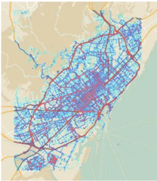
The proposed architecture is validated using real traffic logs from one week of Floating Car Data (FCD) in the city of Barcelona, provided by one of the largest road-assistance companies in Spain, comprising thousands of vehicles from their fleet only in the city of Barcelona. The dataset (further described in Section5.2) comprises data collected over one week between 10/27/2014 and 11/01/2014 across the Barcelona metropolitan area.Fig. 1shows a heat-map of the vehicle tracking data, comprising over 890,000 data samples and a fleet of more than 100 cars moving simultaneously around the city at some times.

Using this FCD dataset, we simulated using the provided FCD across several conditions, from scenarios in which no connectivity failures occurred between the Fog nodes and the Cloud, to scenar-ios with long and frequent connectivity outage periods. For each one of those scenarios, we have analyzed the resilience and accu-racy of the data distribution algorithm and the learning methods.

While current frameworks dealing with FCD analytics focus on how to distribute load towards anomaly detection, modeling and trend prediction on Cloud infrastructures and leveraging Map-Reduce mechanisms to handle traffic data, in this work we focus on (1) the scenario where analytics can be partial or completely performed on the Edge instead of on the Cloud; and (2) the proper transmission of data between Fog nodes on the Edge and the Cloud towards delivering data to be aggregated or learned models to be used. The current case of use targets city-wide traffic data, but Edge-Cloud architectures can be used for enhancing Smart City applications, like power monitoring and control of elements in public spaces, connectivity on demand from smart phones towards public services, or sensor data recopilation from smart phones towards retrieving environmental data [2].

Fig. 1.Barcelona metropolitan area map, combined with a heat-map overlay of the FCD dataset used for the simulations presented in this paper. The dataset contains more than 890,000 data samples of road-assistance cars moving around the city.

Experiments show that the here presented architecture for data distribution running in the Fog nodes is resilient to back-haul con-nectivity issues, and it is able to deliver data to the Cloud location even in presence of severe connectivity problems. Additionally, the proposed traffic modeling and forecasting method based on CBRMs, not only is able to predict telemetry features at short terms but also exhibits better behavior when modeling local data at Fog nodes instead of a centralized model in the Cloud, useful when connectivity issues force data to be delivered out of order to the Cloud, providing an extra degree of autonomy to Fog nodes.

In summary, the three major contributions of this paper are:

•

Data Distribution algorithm for FCD collection in city-wide Fog deployments. The algorithm is designed to be resilient to back-haul connectivity issues, to avoid data to be lost under connectivity outage periods, and to favor distributed data modeling in the Fog. The paper also provides an analysis of the behavior of the algorithm under different scenarios of lost connectivity.

•

A distributed traffic learning and forecasting model, partic-ularly designed for Fog deployments in the city, in which data collected by the data distribution algorithm is fed into a distributed set of Conditional Restricted Boltzmann Ma-chines (CRBM). The neural networks learn traffic patterns across the city and can be leveraged to forecast future traffic conditions. The distributed approach is superior to a Cloud-centralized schema in terms of resilience against network connectivity outages.

•

Validation of the two previous elements through the sim-ulation of different network stability conditions, using as a source real FCD data collected in Barcelona for one week period in 2014.

The paper is structured as follows: Section2 introduces the background on distributed architectures and IoT management. Section3presents the proposed solution towards the current prob-lem. Section4describes in detail the components of the presented approach. Section5shows the different evaluation experiments

(3)

Fig. 2.Fog computing and different levels between Edge and Cloud.

for the current proposal. Section6provides relevant related work. Finally, Section7provides the conclusions and future work. 2. Edge analytics and forecasting with CRBMs

2.1. Analytics on the edge versus cloud analytics

An aspect to consider when computing analytics on the Fog is whether the analytics are performed in the Edge, in the Cloud, or in an intermediate level. Such analytics can be focused on aggregating data (e.g. counting and data-stream analytics), or in characterizing data (e.g. modeling and machine learning analytics for prediction). Computing on the Edge often implies Fog nodes to keep a critical mass of data or partial data aggregations, depending on the complexity of the analytics to be performed, plus enough com-puting power to process data. Otherwise, modeling on the Cloud requires moving data and local aggregations up, then returning the models and analytics if to be used in the Edge, depending on communications but enabling more complex analytics. In those scenarios that data cannot be directly processed on the Edge, but connectivity to the Cloud needs to be economized, intermediate Fog nodes can be enabled in between Edge and Cloud, to collect data and produce aggregated analytics and models. The Fog com-puting paradigm allows the design of a hierarchy of nodes from Edge to Cloud, placing those analytics and modeling processes in the most suitable level according to connectivity and computing power.Fig. 2shows the Fog computing paradigm on aggregation and data processing levels between the Edge and the Cloud.

Furthermore, in scenarios with low amount of data per node, machine learning methods may become under-trained if a critical amount of useful examples is not met, or reaching this amount may take too much time. Then, collecting data in upper levels and the Cloud, could provide much faster a higher amount and more diverse data, with all nodes cooperating to provide a valid training dataset. This would be the case for a model trained from all collected data, or when examples from one node can complement examples from another to avoid model over-fitting situations. On the other hand, scenarios with enough data per node can venture to create machine learning models locally, becoming independent from other nodes or the connection with the Cloud.

Finally, another aspect to consider when computing analytics in the Edge or in the Cloud, is the frequency of updates. While on off-line machine learning methodologies, a training dataset is compiled once to produce a model that is distributed once, on-line machine learning methods require to define update policies indicating the periodicity of model updates and replacements. The advantages of off-line learning is that once the model is created (and distributed if applies), no further operation is required, but

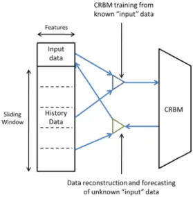
Fig. 3.Schema of CRBM training and prediction.

if data changes over time such models become outdated. The advantages of on-line learning is that models can be created from few or no data, the updated as data keeps coming, but the training process must be periodically repeated.

2.2. Conditional Restricted Boltzmann Machines

In this work we are using Conditional Restricted Boltzmann Machines (CRBM) for modeling and forecasting, a Machine Learn-ing technique proposed by G. Taylor et al. [3]. CRBMs are an extension of a Restricted Boltzmann Machine, specially (but not only) designed to handle sequential data. We chose CRBM among other time series methods because they provide (1) a representa-tive non-simplistic aggregated analytics involving data processing, not as simple as e.g. data-stream sketches and not as complex as e.g. convolutional neural networks or other machine learning ensembles; (2) a method to produce on-line exportable and updat-able models, as the set of matrices composing a CRBM model can be easily transported and re-trained; and (3) the capability for long term forecasting, that might be useful in scenarios where the Cloud requires to estimate the status on the edge but communications are interrupted.

The CRBM modeling presented here uses a Gaussian Bernoulli RBM (GB-RBM) to model the static frames of the input time series. While standard RBMs model only binary data, GB-RBMs are used to handle real and integral valued components. The GB-RBM is an Energy-Based Model with Gaussian visible variables (inputs) and hidden Bernoulli variables (featurized representation). Variables in this type of models are also called ‘‘units’’ or ‘‘neurons’’. We used the GB-RBM configuration as in Taylor’s [3] and Salakhutdinov’s [4] approaches.

Our CRBM models are essentially a GB-RBM with extra inputs to model temporal dependencies. To be specific, to train a CRBM fore-casting model, we keep a history window then feed the model with each current input plusnprevious steps. The training process is done through a Contrastive Gradient Descend [5] iterative process, where each sample (with itsnprevious samples) is seen by the CRBM. Through this, the CRBM learns the relation between input and history, allowing input prediction atkfuture steps, through a Gibbs sampling. The advantage of CRBMs over other methods is that it directly handles multi-dimensional input vectors, also allowing constant updates and retraining.Fig. 3shows the basic CRBM schema.

(4)

CRBMs are used in other fields for characterizing and predicting time series, like in Taylor’s work [6] for human motion modeling or in Cai’s work [7] for financial data modeling, providing enough ex-perimental support to consider CRBMs a proved stochastic method for time series forecasting, with dimensionality reduction capabil-ities and able to be updated on-line.

3. System architecture

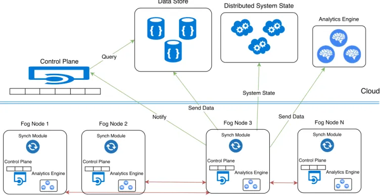
The solution proposed in this paper is based on the Fog com-puting paradigm, combining a data distribution algorithm oriented towards data collection resilient to back-haul connectivity issues, and a traffic modeling approach providing distributed traffic fore-casting capabilities, based on the aforementioned Conditional Re-stricted Boltzmann Machines (CRBM).Fig. 4shows the schematics of the proposed architecture. In this architecture, the Fog nodes (in-cluding nodes in the Edge) implement the control plane, providing the implementation for data collection algorithms and analytics engines (including machine learning modules, here the CRBMs), also the mechanism for pushing data and models towards upper levels and the Cloud. The Cloud level, containing the end-points for the Fog node hierarchy, provides the Data Store with scalability and distribution capabilities, also fault-tolerance mechanisms; the System State monitoring mechanisms, continuously providing sta-tus information for all the architecture components; and analytics requiring global data and high performance computing resources. 3.1. Traffic modeling in the Edge vs. Cloud: tradeoffs

Given the proposed scenario, we consider two approaches when modeling traffic: performing the analytics on the Edge or in the Cloud. Computing models on the Cloud requires collecting all data from Fog nodes, being constrained by possible transmission failures, while computing models on the Edge requires some com-puting power to perform the analytics. As shown inFig. 5, mod-eling requires data susceptible of transmission disruption, or low-powered devices powerful enough, depending on where modeling is taking place.

Location of models also depends on the network capacity and intended use for analytics. One of the purposes of computing on the Edge is to save data transmission by pushing only aggregated (modeled) information to the Cloud. Infrastructure architects must consider the Fog nodes capacity to produce such aggregations, in front of network bandwidth and availability, so more aggregated data towards low transmission volume requires higher computing power, and vice-versa. Further, scenarios requiring analytic models on the Edge, and analytics being aggregated on the Cloud (individ-ualized or generalist models requiring HPC resources), may require models to be pushed back from Cloud to the Fog nodes. Then, those architectures depending on data/model transmissions along time must be aware of back-haul disruption problems.

3.2. Modeling architecture

A model is created by collecting data (from all nodes in the gen-eral model, or from a single node on individual models), training or updating a CRBM able to forecastt

+

1 telemetry data from t

. . .

t

−

dhistory, wheret= time,d= history memory. As the Cloud collects data from all nodes, a general model can be created from all collected data (here location features for each data value are useful), or individual models can be created for each node to spe-cialize them. In Fog nodes, local data is used to create a spespe-cialized model for that node. The CRBM learns and forecasts the following features# cars(volume of traffic during that time interval), and average speed, from previous traffic volume and average speed, also includes information about the location of the Fog node (latitude

and longitude). Further, information about the position of the FCD source is also available, towards discriminating data from specific traffic areas or streets when performing aggregations; while at this time we considered a specific distribution of antennas to dis-criminate traffic areas (heavy traffic streets, residential areas, etc.), when antennas are arbitrarily distributed, data source position is required to perform proper discrimination towards aggregations. Fog node location becomes useful when creating a global model, being able to forecast information from any location.

The CRBM policy on data arrivals require that data is sorted by time-stamp, as usually models learning from time series require. This makes critical for intermediate Fog nodes and the Cloud to receive data in order towards proper aggregation and learning. For empty time-stamp gaps (when no data arrives for a certain time), data is complemented with zeros: entries with the corresponding time-stamp, the last observed latitude and longitude (considering that Fog nodes are fixed in place), and 0 at each other feature. Empty gaps can respond to ‘‘no data emitted’’ or ‘‘data didn’t reach the cloud’’. At this time, from the CRBM at the Cloud point of view, both situations are indistinguishable not knowing if silence is due to a connection failure or no data to be received. So the standard policy is to fill ‘‘not available data’’ with the default values, as we cannot assume any other values. This treated new batch of examples is then split into mini-batches to be fed to the CRBM.

Additionally, CRBMs can be easily updated and re-trained, by iterating over the new provided information. Here we apply an on-line training approach, where new produced data is used to update the models. Either in the general model scenario or the localized models scenario, data is buffered and fed into the CRBM for training periodically. While localized models just keep their models up-dated, the Cloud scenario requires transmitting its models to the edge.Fig. 6shows the updating schema between edge-cloud-edge on the Cloud scenario.

3.3. Data distribution algorithms

One of the principal contributions of this architecture, is the inclusion of a real-time data distribution algorithm with enhanced resilience against back-haul connectivity issues, to avoid data to be lost under connectivity outage periods, and to favor distributed data modeling in the Edge and intermediate Fog nodes.

The algorithm is based on the Fog computing paradigm and node hierarchy between the Edge and the Cloud, to allow data collection and modeling on Fog nodes when suffering connectivity issues, then push data and models towards the Cloud for further analysis and storage when connectivity allows it.

Data distribution among layers is driven by two key algorithms presented as Algorithm1and 2, in charge of the operations for inserting data and pushing data, present on each Fog node. The System State monitor, placed in the Cloud level, is responsible to keep the information of all Fog nodes, including network addresses and connection state, also the overall timestamp of the system. The Cloud and intermediate Fog nodes maintain timestamp tracking in order to flag those batches of data arriving late, this is, belonging to a push request previous to the one in course.

Each Fog node contains its own buffer where data is collected. Nodes collecting data from different nature can possess different buffers, to be processed each one independently from the other ones. For simplicity, here we are showing nodes with one buffer of data, but this process can be replicated for as many data streams as necessarily. Then, each buffer is processed when reaching its capacity.

TheInsert Data Algorithms(Alg.1) is in charge of processing the data incoming into the Fog node. For each stream of data arriving to a Fog node, the algorithm if there is an already existing buffer dedicated to it, otherwise it creates one, and stores data until the

(5)

Fig. 4.Schema of the proposed architecture at Fog level and Cloud level.

Fig. 5.General model in the Cloud vs localized models on the Edge.

Fig. 6.Updating models in the Cloud-training scenario.

buffer is full. Once the buffer capacity is reached, the content is sent to the Data Synchronization Module, where it is prepared to be pushed towards the upper levels. At this point, the overall system timestamp is updated, and all the sibling Fog nodes are requested to process their buffers into their Data Synchronization Modules. At this step, if a node is unreachable, its state changes to ‘‘disconnected’’. After all the registered buffers are processed, the algorithm notifies the Control Plane on the Cloud level or upper Fog node (in the algorithm referred as ‘‘Dispenser’’) that a processing window has been performed.

ThePush Data Algorithm(Alg.2) is in charge of pushing the data when a buffer reaches its capacity, or a Fog node is requested to do that as a result of a sibling node’s buffer reaching its capacity. This algorithm is called from theInsert Data Algorithmwhen the aforementioned conditions are met. On the Cloud level (or inter-mediate Fog nodes), data received from each child node marked as ‘‘connected’’ is processed and flagged as ‘‘ordered’’, while for nodes marked as ‘‘disconnected’’ at some point, the arrival timestamp of the data is checked by comparing its arrival time versus the overall timestamp, then marked as ‘‘disordered’’ if corresponding. For batches of data marked as ‘‘disordered’’, it is responsibility of the analytics engines to decide whether refuse or process them. For the current scenario, CRBMs can decide whether to reorder data to have available as much data as possible, or refuse it avoiding to increase the load on the Cloud or intermediate nodes. Here we decided to maintain the last batches of ordered data as input for the CRBMs.

4. System components

In this section we describe in detail the components that are part of the system architecture described in Section3.

4.1. Fog node control plane

This component runs in each Fog node, in a completely decen-tralized mode. It manages the system state through the use of the distributed system state component described later in this section.

(6)

Algorithm 1Fog node receive data

1: functioninsertData(stream

,

body)

2: Input:Data Stream namestream, Json databody 3: Output:Http Response Status

4: data_array

←

getStreamDataArray(stream)

5: ifdata_array

=

nullthen

6: data_array

←

addStreamDataArray(stream)

7: setStreamState(stream

,

Config

.

ip)

8: end if

9: data_array

.

putDocument(body

,

timestamp)

10: ifdata_array

.

full()then

11: pushBuffer(data_array

,

state

,

stream)

12: updateTmstp(stream

,

timestamp)

13: for allnodeinstate

.

nodesdo

14: node

.

pushBuffer(node

.

stream

.

data_array

,

node

.

stream

.

state

,

stream)

15: iferrorthen

16: setStreamState(stream

,

node

,

false)

17: end if

18: end for

19: Dispenser

.

postCollect(stream

,

tmstp)

20: end if

21: returnHttp

.

Status(201)

22: end function

Algorithm 2Fog node push buffer data function

1: functionpushBuffer(data_array

,

state

,

stream)

2: Input:Node data arraydata_array, node statestate, Data Stream namestream

3: ifstate

.

connectedthen

4: storeArrayOfData(data_array

,

stream)

5: else

6: for alldataindata_arraydo

7: created_at

←

data

.

get(created_at)

8: ifcreated_at

>

state

.

tmstpthen

9: storeData(data

,

stream

,

true)

10: else

11: storeData(data

,

stream

,

false)

12: end if

13: end for

14: end if

15: end function

It is implemented as a web component that can be interfaced using REST APIs, and it implements the core algorithms described in Section3.3. The REST APIs are composed of a Servlets Container and a REST Engine. As a HTTP Web Server and Java Servlet container we use Jetty [8], which is a pure Java-based HTTP server and Java Servlet container. Jetty is often used for machine-to-machine communications, usually within larger software frameworks. As a REST Engine (JSON processor) we use Jackson [9], which is a high-performance suite of data-processing tools for Java, including the flagship JSON parsing and generation library, as well as additional modules. The Jackson Project also has handlers to add data format support for JAX-RS implementations like Jersey.

4.2. Data store and data synchronization module

A distributed data store is used to keep track of all the Fog nodes produced data. For that purpose, CouchBase [10] has been chosen because it provides the benefits of NoSQL data stores (highly distributed, high-availability properties, scalable), and it is document oriented (which fits well for many different data sources and formats). Queries on the data are available using a query DSL.

The mechanism to send queries to the platform has been integrated in the API that resides in the central Cloud location.

The data synchronization between Fog nodes and Couchbase is done by the Data Synchronization Module that is deployed with CouchBase Mobile [11]. Couchbase Mobile is composed of Couch-base Lite [12], an embedded database that manages and stores data locally on the Fog nodes, and the Sync Gateway [13] that provides synchronization between Couchbase Lite and Couchbase Server.

Couchbase has native support for JSON documents. Each JSON document can have a different structure, and multiple documents with different structures can be stored in the same CouchBase bucket. Document structure can be changed at any time, without changing other documents in the database. A Bucket is defined as the owner of a subset of the key space of a Couchbase cluster. These Buckets are used to distribute information effectively across a cluster. A Bucket is equivalent to a database. A common practice is to store documents of different nature on different buckets. The architecture has the ability to store different data nature in different buckets via the Control Plane in the Fog nodes. For the work presented in this paper we have defined one bucket since all the data have the same nature.

4.3. Managing the distributed system state

System State is the module that provides the information on the status of all the components of the architecture at all times and is implemented using etcd [14]. Etcd is a distributed reliable key– value store that is automatically replicated with automated master election and consensus establishment using the Raft algorithm, all changes in stored data are reflected across the entire cluster, while the achieved redundancy prevents failures of single cluster members from causing data loss. Etcd also provides service dis-covery by allowing deployed applications to announce themselves and the services they offer. Communication with etcd is performed through an exposed REST-based API, which internally uses JSON on top of HTTP.

4.3.1. Analytics engine: local in fog nodes or global in cloud

Both Fog nodes and Cloud have a module for performing the proposed analytics. Such module is in charge to buffer the data for training and updating CRBM models, store the current CRBM model in each situation, forecast data using the models, also to transmit models from Cloud to Fog nodes using the aforementioned REST API. Both Fog and Cloud nodes have available the same implemen-tation, ready to receive data for training/updating or forecasting, and to produce or receive a trained model. The analytics framework is hooked to the data stream, buffering data for periodic model updates. Once a model in the Cloud is trained or updated, it is transmitted to the corresponding Fog nodes. If the model is trained or updated in the Fog nodes, models are kept locally, as explained previously in Section3.2.

The analytics and machine learning framework for training CRBMs is created using R from the Comprehensive R Archive Net-work [15]. The implementation of the CRBM methods is obtained from our implementation in R,1 based on the G. Taylor’s original approach. Communication between the REST API and the analytics is built using the package R-Plumber [16]. While R-Plumber man-ages the connections between API calls and handler functions, the well-known R packages JSONlite [17] and HTTR [18] are used to serialize CRBM models (a set of matrices) and transmit them.

(7)

5. Evaluation

In this section we present 5 different experiments that illustrate the behavior of the data distribution algorithms and the traffic modeling component. Across the different experiments, we show how the Cloud-centric learning strategy can lead to incomplete datasets passed along to the analytics engine. This, in turn, results in biased and inaccurate models due to potential back-haul con-nectivity issues. Therefore, the experiments show the advantages of a decentralized Fog-based learning strategy to improve the accuracy of the models and protect the system against connectivity outages.

5.1. Methodology

The data distribution layer was tested under two different con-ditions: internal memory buffers of 100 elements (small buffer, continuous synchronizations between the Fog node layer and the Cloud components), and 10,000 elements (large buffer, reduced communication patterns between the Edge and Cloud).

Deployed antennas cover different traffic areas where traffic can be aggregated by coverage zone (using all received data), or by traffic zones (discriminating received data by data source loca-tion) if specific streets or delimited traffic areas are to be studied separately. Here we emulated six different antennas (and their corresponding Fog nodes), distributed across the metropolitan area of Barcelona, covering each a different traffic area. Some of the coverage areas are slightly overlapped to guarantee that all the territory got covered by at least one antenna. In all experiments, the FCD data was traversed over time, re-creating the original sequence of events. At each step, data sample was sent to its corresponding nearest antenna. The distribution of data across each Fog node for a configuration corresponding to a node local buffer size of 100 data samples can be seen inFig. 7.

Different patterns of network connectivity issues between the Fog nodes and Cloud components were emulated. Network failures were modeled using a mean time between failures that follows a random LogNormal distribution. Different configurations were used, with mean values of 20, 30 and 40 min between failures.Fig. 8

shows the actual time between failure distribution used in the experiments. We also modeled the duration of each connectivity failure: in this case, we considered another LogNormal distribution with mean value of 10 min.

Finally, we also modeled the number of nodes affected in every connectivity outage, In this case, an exponential distribution was used for each node, resulting affected all nodes with values above 0.5 (namely,low impact scenario). We also considered a second case in which the impact of each failure was significantly higher, representing an scenario in which extreme connectivity issues affect the city. For that scenario, the threshold to decide if a node was affected by the backhaul connectivity outage was set to 0.2 (namely,high impactscenario).

5.2. Validation dataset

With the purpose of validating the current architecture, we have chosen a traffic monitoring and prediction case of use, for a set of 118 vehicles reporting their speed to the Fog node at different moments. We are using real traffic logs from around one week of ‘‘Floating Car Data’’ (FCD) collected in the city of Barcelona, monitoring the traffic in 6 different locations, with 45094 records for 6 days. The collected features include, for each specific Fog node, the number of cars reporting their presence to each node and the average speed for those cars, also each record also includes the position for the Fog node collecting it, and the timestamp. The two most relevant features to be learned and forecasted are traffic

volume and average speed, with an average of 9 cars per record and between of 1 to 47 (when no cars are reporting, no record is included in the dataset), and average mean speeds of 19 km

/

h and values between 0 km

/

h and 124 km

/

h. Notice that records with speed limits higher than 60 km

/

h are in the 99th percentile so we can consider them outliers to prevent them to alter our analytics (also technically the maximum allowed speed in the city is 50 km

/

h); reducing those records withspeed

>

60 to just 60 keeps the average mean speed to 19 km

/

h and values between 0 km

/

h and 60 km

/

h.

5.3. Evaluation infrastructure

The experiments were run in a cluster of 8 servers, each fea-turing two Xeon E5-2630v4 (broadwell) processors, clocked at 2.20 GHz. Each node counts with 128 GB of DDR4-2400 R ECC RAM. All nodes were interconnected using a non-blocking 10GbE switching fabric. Although an external NFS folder was mounted on the systems, it was not used as a backend for the experiments. Instead, all data was stored locally using four 7.2K rpm 2TB SATA HDDs per nodes, mounted as four independent volumes.

The application was deployed using Docker [19] containers that encapsulated every system component. Docker containers provided all the necessary elements for the evaluation: network isolation, communication and network connectivity control of ev-ery component that runs as an isolated process.

5.4. Experiment 1: Percentage of generated data available in cloud In this first experiment we perform an exploratory analysis of the architecture behavior and algorithms, from the point of view of the ratio of the data available in the cloud (stored in the Data Store) versus the data processed on the Fog nodes.

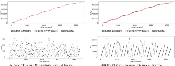
Figs. 9(a)and9(b)show the cumulative data processed along the time by the Fog nodes and stored in the central Cloud for buffers of 100 and 10k items respectively. As it can be observed, for larger buffers there is a slight sawing in the graph because until the buffer is not filled and launches the processing of all the nodes, which takes more time than for smaller buffers, the processed data will not upload to the Cloud.

From the point of view of the difference between the data generated and the data available in the Cloud,Fig. 9(d) shows this effect of buffer filling more clearly showing in a linear way the increase of the difference until it falls through the buffers processing.Fig. 9(c) validates that the difference between data generated versus data available in the cloud is small for smaller buffers, for this reason the effect of the buffer processing is blurred. Notice thatFigs. 9(a)and9(b)are not linear, for the reason that there is less data volume at night.

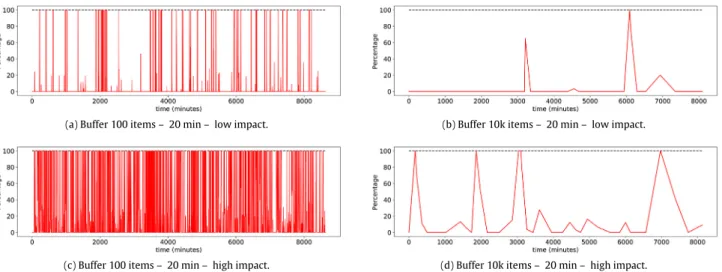
5.5. Experiment 2: Impact of connectivity issues — data affected In this second experiments we visualize the amount of data affected by connectivity issues, and therefore delayed more than desired, on the proposed scenarios, showing how in some oc-casions percentage of losses continuously reaches 100%, always depending on the buffer dimensions. This is the data that at some moment could not be delivered to the Cloud when expected either because the node was disconnected when it went to process its full buffer or because it could not be notified by another node to process it. Realize that may include data delivered in order and data not delivered in order.

Figs. 10(a)and10(b)show the percentage of data affected by connectivity issues with a frequency of next failure of 20 min for Fog nodes with buffers of 100 versus buffers of 10k items. As can be seen, with larger buffers there is less affected data, this is due to the

(8)

(a) Fog node 1. (b) Fog node 2.

(c) Fog node 3. (d) Fog node 4.

(e) Fog node 5. (f) Fog node 6.

Fig. 7.Data processed by each Fog node with 100 buffer items.

(a) Failure frequency — 20 min. (b) Failure frequency — 30 min. (c) Failure frequency — 40 min.

Fig. 8.Distribution of actual connectivity outages simulated between the Fog nodes and Cloud layers. It follows a random LogNormal distribution.

(a) Buffer 100 items – No connetivity issues – accumulate. (b) Buffer 10k items – No connetivity issues – accumulate.

(c) Buffer 100 items – No connetivity issues – difference. (d) Buffer 10k items – No connetivity issues – difference.

Fig. 9.Representation of data in Cloud over time without connectivity issues. Increasing buffer sizes in Fog nodes, the communication pattern between the Fog nodes and the Cloud is changed, with less frequent but more intense network traffic bursts when the buffers are larger, and at the same time, delays in propagation are also increased (Experiment 1).

(9)

fact that there is less volume of buffer processing and therefore less probability that the Fog nodes are disconnected at that moment. On the contrary, with smaller buffers many times more than the buffer is processed the Fog node is disconnected.

Figs. 10(c)and 10(d)show the percentage for the same fre-quency of next failure (20 min) but incrementing the number of nodes failing. As described in Section5.1, this is done modifying the random exponential function decision value. Incrementing the number of failing nodes to reach a high impact situation can be observed as for small buffers the effect is much greater that for larger buffers. The density of affectation is also greater between nodes with the same buffer size,Figs. 10(a)and10(c)more affected than forFigs. 10(b)and10(d).

5.6. Experiment 3: Impact of connectivity issues — data delivered out of order

In this third experiment, we revisit again the data loss ratios in different scenarios, considering only the data delivered out of order from the point of view of the Cloud. The evaluation carried out in this experiment accounts only for the sets of data that could not be delivered in order, this is important for cloud analytics because it can be used to define confidence intervals on existing data in the data warehouse. Notice that the amount of data disordered will be always less than the data affected by connectivity issues (Experiment 2) because is not taken into account the data in the buffers when a Fog node has to process its full buffer and it is disconnected.

Figs. 11(a)and11(b)show the percentage of data disordered with a frequency of next failure of 20 min for Fog nodes with buffers of 100 versus buffers of 10k items. As in Experiment 2, with larger buffers there is less disordered data due to the less volume of buffer processing and with smaller buffers more disordered data reach the Cloud.

In the same way, under a high impact situationFigs. 11(c)and

11(d)show the same behavior as Experiment 2, for smaller buffers the disorder is much greater that for larger buffers. The density of disorder is also greater between nodes with the same buffer size

Figs. 11(a)and11(c)more affected than forFigs. 11(b)and11(d). As previously explained if overall density between this Exper-iment and ExperExper-iment 2 is compared the density in the figures in Experiment 2 are greater.

5.7. Experiment 4: Impact of connectivity issues — data contaminated by out of order deliveries

In this experiment we evaluate all data that has been affected by out of order delivery, directly or indirectly. Here we account the amount of data that has been contaminated (incorrect mix will lead in bad training) either because it was delivered out of order or because other data that should have been mixed with it could not be pushed on time. This is important, not for real time, but to support the idea that building models in the Fog nodes are much more accurate that building models in the Cloud.

Following the evaluation of the previous experiments (Exper-iment 2 and Exper(Exper-iment 3), Figs. 12(a)and 12(b) show with a frequency of next failure of 20 min for Fog nodes with buffers of 100 versus buffers of 10k items the percentage of data affected. The data with larger buffers there is less affected than smaller buffers due (as in previous experiments) to the less volume of buffer processing.

As previous experiments, under high impact situationFigs. 12(c)

and12(d)show for smaller buffers much more affectation than

for larger buffers. Coherently with the rest of experiments . The density of affectation is also greater between nodes with the same buffer sizeFigs. 12(a)and12(c)than forFigs. 12(b)and12(d).

This experiment presents the highest density of affected data compared with Experiment 2 and Experiment 3. The amount of data contaminated by out of order deliveries, directly or indirectly is the highest.

5.8. Experiment 5: Traffic modeling and forecasting. centralized vs distributed

Here we evaluate the modeling and forecasting methodology, to validate how the proposed architecture allows modeling the input data. As previously explained, the principal case of use consists on predicting road traffic properties (i.e. volume of traffic and average speed) per Fog node. We considered two different scenarios: a centralized training process where all data is collected to create one general models, and a distributed training process where each Fog node produces its local model.

In the following experiments we consider the scenario where data is collected on the Cloud and a CRBM model is created, and the scenario where the CRBM is trained in the Fog nodes. While the first scenario considers no connection failures, becoming the best scenario, the second considers that local models are independent to the ratio of connection failures. In case of no failures, the both scenarios could be performed on the Cloud: a global model and individual models for each node from received data. In case of failures, we can rely on locally trained models, not depending on failures. Then here we show how a global model behaves versus local models.

The CRBM has been tuned after repeated experiments looking for the best hyper-parameters, here hidden units = 30, learning rate = 0.01, momentum = 0.8 and number of training epochs = 4000, also data is aggregated in vehicles and average speed per hour. The historical window kept for prediction is 3 h, and the forecasting is produced through 30 iterations of Gibbs sampling.

Warm up time for initial CRBM training, also CRBM update (re-training) periodicity is set up to 24 h, after experimenting with different periodicities, being 24 h the best update interval. Note that real data displays a daily (24 h) repetitive pattern, so training the model each 24 h ensures a fairly balanced set of observations. Additionally, the speed limit has been limited to 60 km/h (99 percent of observations) to neutralize outliers (for alls

>

60, it is set to 60), also noticing that maximum speed allowed inside the city is 50 km/h, and those values could be considered towards anomaly detection for traffic law enforcement in future works.

Table 1 shows (on the two top tables) the average Relative Absolute Error (RAE, a.k.a. Mean Absolute Percent Error) for each node using a global model, trained and updated using all nodes information, against using local models for each node, trained and updated only with local data. We distinguish the complete error and the 95th percentile error, where we focus on the error for the 95 percent of cases, as we observed that the error distribution produces a long tail, altering the perception of the expected error. As CRBM has a stochastic component, experiments have been run 10 times, and computed the average of results.Fig. 13also displays the averaged values in right column for better comprehension.

We observe that local models produce better predictions than a general model, indicating that each node has enough data for itself to train a decent predictor. Such effect would allow a single node to train or update its CRBM model in case of disconnection from the cloud. On the other side, management systems on the cloud could use the CRBM model to estimate the telemetry from the disconnected Fog node. Notice that the error varies per node, as each node registers information from a different part of the city: nodes 3 and 4 are located in the periphery, receiving less data than the others and benefiting from the general Cloud model.

Finally, to conclude the modeling evaluation, we consider how communication failures affect the centralized modeling in the

(10)

(a) Buffer 100 items – 20 min – low impact. (b) Buffer 10k items – 20 min – low impact.

(c) Buffer 100 items – 20 min – high impact. (d) Buffer 10k items – 20 min – high impact.

Fig. 10.Fraction of data sitting in the Fog node Layer is affected by back-haul connectivity issues over time. Simulated time between errors following a random LogNormal distribution with mean values 20 min. May include data delivered in order and data not delivered in order to the Cloud. In Low impact scenario, few Fog nodes are affected by the connectivity issues. In the high impact scenario, the scope of connectivity outages is larger (Experiment 2).

Fig. 11. Fraction of data sitting in the Fog node Layer that is deliveredout-of-orderto the Cloud layer because back-haul connectivity issues over time. Simulated time between errors following a random LogNormal distribution with mean values 20 min. Only includes data not delivered in order to the Cloud. In Low impact scenario, few Fog nodes are affected by the connectivity issues. In the high impact scenario, the scope of connectivity outages is larger (Experiment 3).

Cloud, by considering that the same aforementioned failure con-ditions apply, ‘‘destroying’’ part of the training/updating datasets. Here we consider that the analytics module is not bound to delayed data synchronization: CRBMs are trained/updated with real-time available data, and data dispatched late (from previous iterations) is discarded, as considering it would imply to keep extra amount of historic data because of the training pre-processing sorting and completing data.Table 1shows also (in the four bottom tables) the relative absolute error for traffic volume and average speed prediction (for all error and error 95th percentile), for scenarios where the average time to failure is

⟨

15

,

20

,

30

,

40

⟩

versus a no-failure scenario, with an average of 10 min of no-failure and expo-nential chances for a node to be affected. As failures are stochastic, experiments have been run 10 times, and computed the average of results.

As we can see, the error degrades with higher chances of failure. We must take into account that given the several rounds of up-dates, CRBMs are able to recover from unseen data up to a certain point, depending on the variability of data in each node and the frequency of failures.

5.8.1. Performance at the Edge

Devices at the Edge are characterized by low consumption and limited performance, as the Fog paradigm focuses on moving high performance computing to the Cloud while ‘‘low cost’’ operations like aggregation and filtering to the Edge. Machine learning mod-eling and prediction can require high or low amount of resources depending on the used method and the amount of data to be pro-cessed. The used CRBMs have the characteristic of being reasonably easy to train in terms of complexity, as data can be split in mini-batches to be passed by the network then computed the gradient difference, i.e. matrix multiplications and subtractions subject to the size of data and CRBM hidden units, then each piece of data is passed enough times until achieve an acceptable accuracy level. As mentioned before, the CRBMs for the current traffic data require 30 hidden units and less than 4000 iteration to achieve lowest error values.

In order to test the viability of the proposed method into a low performance environment for machine learning and aggregations, we have deployed the framework into Edge devices composed by Raspberry Pi 3B (Raspi) micro-computers, with computing power of 4xARM Cortex-A53 @1.2 GHz and 1GB RAM memory, with peak

(11)

Fig. 12.Fraction of data sitting in the Fog node Layer that is delivered inincomplete stateto the Cloud layer because backhaul connectivity issues over time. Data delivered in incomplete state is data that although it is delivered in-order to the Cloud, it contains missing parts that could not be delivered in time. This aspect is important because learning models can get biased because of lack of completeness in the data seen. Simulated time between errors following a random LogNormal distribution with mean values 20 min. Only includes data delivered in order to the Cloud, but with missing parts. In Low impact scenario, few Fog nodes are affected by the connectivity issues. In the high impact scenario, the scope of connectivity outages is larger (Experiment 4).

Fig. 13.Average RAE for values onTable 1.

power consumption 3.7 W (730 mA). Each Raspi is prepared as a Fog Node receiving data from a given coverage area.

As showsTable 2, aggregating collected data in rounds of 1 h and re-training local CRBM models in round of 6 h, require less than 25% of a CPU and

∼

21 KBytes of RAM memory to aggregating and training data, and times are below 5 s to perform the process of aggregation and training, also predicting the new batches of data using the local model. Take into account that the impact of the amount of input data affects uniquely the Aggregation process and Prediction process, as the CRBM models receive data normalized in fixed time-steps.

5.8.2. Discussion on modeling

Complex policies can be developed in the future like multi-level training if needed, where models are created on the Cloud and

also locally or intermediate nodes, and in case of failures Cloud models are selectively discarded when transmitted to Fog nodes, local models are pushed to the Cloud to update the centralized ones, or intermediate models are distributed up and downwards. Here we shown that models can be trained in the Cloud from all data, also in lower levels from local data.

In scenarios where partitions can change behavior along time and models need to generalize, being trained with low probability situations to learn about patterns not seen by it but by others, helps to create a non-over-fitted model with less precision but more accuracy. However, in practice, this is something hard to achieve. As seen in the experiments, local models tend to over-fit to their local samples, usually performing better than global ones. So in case Fog nodes are capable to perform the modeling as part of their analytics, another policy would be to train at the edge then push local models to the Cloud for centralized management purposes, and only re-train models on the Cloud for those nodes benefiting from extra data.

It is also in our road-map to plan scenarios where Fog nodes may change location or move (e.g. Fog nodes on vehicles). So contemplating a policy where local models can be updated with past data from other nodes in that location could improve them. 5.9. Summary of results

The following is a summary of the most important aspects of the results presented in this Section:

•

Experiment 1: Shows the behavior of the data distribution algorithm in terms of amount of data collected by the Fog nodes and not available at the Cloud level. This factor is conditioned by the size of the buffers in the Fog nodes, that in turn translate into delays in propagating data to the Cloud. At the same time, increasing buffer sizes, the com-munication pattern between the Fog nodes and the Cloud is changed, with less frequent but more intense network traffic bursts when the buffers are larger.

•

Experiment 2: Shows the impact of network connectivity issues between the Fog nodes and Cloud layers, resulting in limited data propagation capabilities during the con-nectivity outage periods. This aspect is evaluated in terms of percentage of data sitting in the Fog node layer that is

(12)

Table 1

Average RAE (for all data and 95th percentile) on collected-data modeling vs local modeling, per node (top tables). Average RAE for forecasting on failure scenarios (bottom tables).

Number of received inputs from each Fog node

node1 node2 node3 node4 node5 node6 Total

8614 8613 5614 5712 8575 7966 45094

Centralized modeling (One general model)

node1 node2 node3 node4 node5 node6 Average

Traffic volume 0.1830406 0.5640958 1.0406101 0.9656460 0.6329655 0.7736946 0.6933421

Average speed 0.5876019 0.4058793 1.7793430 0.4139850 0.3334604 0.3530163 0.6455477

Traffic volume (95th) 0.1706984 0.5323832 0.8967587 0.8716846 0.5885903 0.6971613 0.6262127

Average speed (95th) 0.5089208 0.3332018 1.1704180 0.3400571 0.2810072 0.2700172 0.4839370

Fog node modeling (One model per node)

Traffic volume 0.1555855 0.5851258 0.6656879 0.6936570 0.6192713 0.7624275 0.5802925

Average speed 0.5436164 0.2711187 1.8857050 0.3521620 0.2454030 0.3343151 0.6053867

Average speed (95th) 0.4206425 0.2248818 1.4680658 0.3243317 0.2126657 0.2462449 0.4828054

Centralized modeling (Avg time to failure 40 min)

Traffic volume 0.2886579 0.5971364 1.326132 1.1623673 0.7139560 0.8785106 0.8277935

Average speed 0.6542469 0.4493091 1.675766 0.4447477 0.3855491 0.3717311 0.6635583

Average speed (95th) 0.5307863 0.3588561 1.193760 0.3657113 0.3242667 0.2837089 0.5095150

Traffic volume 0.3047327 0.6216623 1.322312 1.1202736 0.6978688 0.8440265 0.8184793

Average speed 0.6367097 0.4329232 1.609276 0.4533244 0.3696029 0.3841081 0.6476574

Average speed (95th) 0.5204882 0.3461248 1.233979 0.3884334 0.3201640 0.3288929 0.5230137

Traffic volume 0.3720164 0.6402134 1.354118 1.0958144 0.7135374 0.8028318 0.8297553

Average speed 0.6804612 0.4302883 1.746649 0.4494588 0.3640312 0.3713571 0.6737076

Average speed (95th) 0.6023073 0.3551524 1.210088 0.3834238 0.3073565 0.3230715 0.5302333

Traffic volume 0.3622710 0.6315523 1.305127 1.1988274 0.7254418 0.7950532 0.8363788

Average speed 0.6991176 0.4623524 1.757799 0.4513180 0.3718768 0.3693187 0.6852970

Average speed (95th) 0.5895197 0.3799004 1.317271 0.3986128 0.3206143 0.3012697 0.5511980

Table 2

Average computing resources and time spent per Edge process, given hourly aggregation and prediction rounds, and 6 h re-training rounds, in each Fog node.

Data Processing Time (seconds) # of Inputs Resources

Aggregating Prediction Training CPU (%) MEM (KB)

Fog node 1 0.07392797 0.09089618 3.776131 1434.8 15.75 20.8906 Fog node 2 0.07263155 0.08739262 3.765014 1434.6 16.22 20.5495 Fog node 3 0.06041346 0.08531480 3.745345 867.2 16.67 20.7227 Fog node 4 0.06405849 0.08406520 3.005376 962.6 17.14 21.5156 Fog node 5 0.07629604 0.08889236 3.762398 1427.2 17.55 21.6471 Fog node 6 0.07259803 0.08957825 3.762089 1313.6 18.00 21.8542

affected by the connectivity issues. Data affected is, at least, delayed on its delivery to the Cloud layer. The importance of this aspect for the Traffic modeling components of the application is that it may delay the model training process in the case of using a Cloud-centric modeling strategy, what is expected to have limited impact in the overall system. The Fog-centric model is not affected.

•

Experiment 3: Similar to the previous experiment, in this case we explore what is the fraction of data that could not be delivered in order to the Cloud layer. A set of data is not delivered in order when other sets of data, both produced by the devices in the edge during the same time range, are not delivered to the cloud in the right order (being the out-of-order set delivered after the other sets). The importance of

(13)

this aspect for the Traffic modeling components of the appli-cation is that it may degrade the quality of the trained model in the case of using a Cloud-centric modeling strategy, what is expected to have moderate impact in the overall system. The Fog-centric model is not affected.

•

Experiment 4: Similar to the previous experiment, in this case we explore what is the fraction of data that was deliv-ered in incomplete state to the Cloud layer because of the sets that could not be delivered in time. A set of data is in in-complete state when it is exposed to the trained model with-out all the sets that were generated in a given time range. The importance of this aspect for the Traffic modeling com-ponents of the application is that it may produce a severe bias in the trained model in the case of using a Cloud-centric modeling strategy, what is expected to have severe impact in the overall system. The Fog-centric model is not affected.

•

Experiment 5: Provides insights on the actual model accu-racy across different scenarios, both for the Cloud-centric and the Fog-centric learning strategies. Results show that the Fog-centric approach is more accurate and at the same time more robust than the Cloud-centric approach, capable to be performed in low computing-power devices.

6. Related work

Several cities around the world are involved in projects towards smart-city management. Platforms designed for management of smart cities exist in cities like Nice, France, where the Connected Boulevard [20] platform has been developed to optimize all as-pects of city management, including parking, traffic, street light-ing, waste disposal, and environmental quality. Also in Santander, Spain, the project SmartSantander [21], focuses on a European facility for research and experimentation of architectures, tech-nologies and applications for smart cities, but without focusing yet on Fog computing. Further, other cities like Songdo (South Korea), Masdar City (Abu Dhabi, UAE), Paredes (Portugal), Manch-ester (UK), Boston (US), Tianjin (China) and Singapore, announced smart-city related projects [22]. Although approaches differ on each city, resilient and secure analytics between the edge and data centers are a hot topic, revolving around a coherent and affordable way of management [23]. In our previous work [2], we focused on how Fog computing architectures can improve the deployment of distributed commercial solutions on smart cities where cloud models fall short, through a Barcelona Supercomputing Center and Cisco Systems joint initiative towards a Fog computing deployment in the city of Barcelona.

The appearance of Floating Car Data (FCD) as data source is expected to provide support to many practical use cases in the near future, leveraging Intelligent Transportation Systems teleme-try. To complement the current lack of sensorization in cars and communications infrastructure, works like [24] propose the use of smartphones and Wi-Fi hotspots, also [25] proposes crowdsourc-ing architectures to collect data from smart devices on vehicles for these same purposes, or [26] studies vehicle-to-vehicle networks to handle the expected escalation of FCD data volume.

In the field of treating Floating Car Data, we find works like [27] where the framework RTIC-C presents a high level architecture to deploy traffic analytics, using Map-Reduce approaches for dis-tributing modeling and processing algorithms. The RTIC-C authors defend the use of big data analytics on traffic data due to its increasing volume and complexity, then they focus on distributing received data for processing on anomaly detection and traffic trend prediction. Our presented framework focuses on the data transmis-sion architecture towards receiving traffic data streams properly for being ingested by analytics methods, i.e. localized re-trainable

CRBM prediction mechanisms, and could complement high level frameworks like those named here on generalist model scenarios. Further, while most state of the art frameworks focus on cessing traffic data on dedicated HPC Cloud infrastructures, we pro-pose to study scenarios where analytics are partial or completely processed in the Edge. Works like [28] and [29] present different traffic modeling approaches, ensembles using bagging and Feed-Forward MLP Neural Networks the prior and Spatial–Temporal Weighted k-Nearest Neighbor the later, producing general models from the aggregated datasets and distributing computation on the Cloud. Also, works like [30] present a methodology where a Stack of AutoEncoders is applied for traffic flow prediction at different granularities with good results for t+1 forecasting. As presented in our work, localized models on the Edge can create in-situ special-ized predictors adapted to their coverage area, using re-trainable machine learning models.

Many Fog applications (e.g. event monitoring and forecasting, as is the case on the presented work), rely on data stream pro-cessing analytics. [31] presents general models and architectures for Fog data streaming, and analyze the common properties of the most common applications. An overview about device-to-device communication on the Fog can also be found in [32], focusing on the physical plane of such devices. [33] shows how connectivity issues are important in this field, specifically in wireless commu-nications, applying an algorithm to prioritize which of the available data in a given field with interconnected sensors is send to a mobile carrier and how to route it when connections between data provider and the mobile carrier are intermittent and short in time. The use of machine learning for time series on Fog computing infrastructures and smart cities is relatively new, although data mining on the Internet of Things has been previously planned and discussed, e.g. [34] proposed the different layers of data manage-ment on IoT analytics: data collection, data managemanage-ment, event processing and data mining. Also applications of ML management on cities already exists that could easily benefit from edge com-puting: from management of power grids using machine learning in big cities from grid monitored data [35], to reduction of data transmission in health-care monitoring wearables by performing pattern mining on the edge [36], to illustrate some examples. 7. Conclusions and future work

Among the new technologies emerging around the Internet of Things (IoT) to provide a new whole scenario for Smart City services, Fog nodes become potential hosts for lightweight services on near real-time close to the edge. Thanks to modern high band-width networks, those previously centralized services can become decentralized, adapting to the constant changes on modern cities without compromising fidelity towards centralized management and data warehousing systems.

Here we presented a decentralized application towards smart-cities traffic monitoring and forecasting. Our architecture com-bines a data distribution layer, connecting the Fog nodes with a centralized Cloud focusing on resilience and near real-time com-munication, and an on-line Machine Learning modeling technique to learn and predict traffic telemetry. The application is designed to be deployed in a Fog-based infrastructure, in which network antennas (e.g. 5G stations) are combined with Fog nodes to provide near real-time computing capabilities.

We have validated and tested the presented approach through five experiments, illustrating the behavior of the data distribution algorithm plus the traffic modeling analytics methodology. And more important, here we are providing evidence of the need for a decentralized Fog-based learning strategy, to improve the accuracy of the trained models and to protect the system against back-haul connectivity issues. We observed that, when a centralized cloud-based approach is followed, network connectivity outages limiting