Fault classification in power systems using EMD and SVM

ELECTRICAL ENGINEERING

Fault classification in power systems using EMD

and SVM

N. Ramesh Babu

_{, B. Jagan Mohan}

School of Electrical Engineering, VIT University, Vellore, India

Received 16 April 2015; revised 3 August 2015; accepted 17 August 2015

KEYWORDS Fault classification; Empirical Mode Decomposition (EMD); Support Vector Machines (SVMs)

Abstract In recent years, power quality has become the main concern in power system engineering. Classification of power system faults is the first stage for improving power quality and ensuring the system protection. For this purpose a robust classifier is necessary. In this paper, classification of power system faults using Empirical Mode Decomposition (EMD) and Support Vector Machines (SVMs) is proposed. EMD is used for decomposing voltages of transmission line into Intrinsic Mode Functions (IMFs). Hilbert Huang Transform (HHT) is used for extracting characteristic fea-tures from IMFs. A multiple SVM model is introduced for classifying the fault condition among ten power system faults. Algorithm is validated using MATLAB/SIMULINK environment. Results demonstrate that the combination of EMD and SVM can be an efficient classifier with acceptable levels of accuracy.

Ó2015 Faculty of Engineering, Ain Shams University. Production and hosting by Elsevier B.V. This is an open access article under the CC BY-NC-ND license (http://creativecommons.org/licenses/by-nc-nd/4.0/).

1. Introduction

One of the main problems for the industry and electrical equip-ment is power quality disturbances such as voltage sag, har-monics. Among all, voltage sag is more dangerous. One of the main causes for voltage sag is short circuit faults such as single line to ground, line to line, and three phase faults. With-out proper classification of these faults from healthy condi-tions, it may cause irrecoverable economic effects. Selecting a

proper algorithm for analyzing these system data for faulty conditions in terms of voltage sag is crucial. An algorithm is needed for pre-processing and extracting most significant fea-tures from the voltage or current data from system under study. These features can be used for detection of the faulty condition among various possibilities. A classifier is needed for this purpose.

Over the years, wavelet transforms are used for analyzing the fault data. Wavelets and artificial neural networks (ANN) are introduced in power system fault detection in the literature [1]. Online applications of wavelet transforms to power system relaying are presented in the literature [2,3]. Classification of causes for voltage sag using wavelet transform and probabilistic neural network is proposed in the literature [4]. Literature [5] introduces wavelet based combined fuzzy logic classifier for power system faults. In these papers wavelets are used for extracting features from power system data with either ANN or fuzzy logic for classification. Support vector machine is emerged as a new classifying approach besides * Corresponding author. Tel.: +91 416 2202467, mobile: +91

9443030636.

E-mail addresses: [email protected] (N. Ramesh Babu), [email protected](B. Jagan Mohan).

Peer review under responsibility of Ain Shams University.

Production and hosting by Elsevier

Ain Shams Engineering Journal (2015)xxx, xxx–xxx

Ain Shams University

Ain Shams Engineering Journal

www.elsevier.com/locate/asej www.sciencedirect.com

ANN and fuzzy logics in recent years. SVM classifier is introduced as classifier for power system faults in[6]. A com-bination of wavelet and SVM for fault classification is pro-posed in[7,8]. Instead of wavelets, EMD with HHT is being used recently for feature extraction stage. Application of HHT and neural networks in detecting power quality distur-bances is presented in [9–11]. Various theoretical parameters to be considered for using HHT and EMD for various appli-cations are presented in[12–14].

A combination of EMD and SVM algorithms for feature extraction and classification of power systems fault is discussed in[15]. In this paper, only classification is done among single line to ground, line to line, double line to ground and three phase faults. In this paper, exact classification among faulty phase and fault type among ten faults (AG, BG, CG, AB,

BC, CA, ABG, BCG,CAG, and ABCG) is calculated. Time of the fault is calculated using instantaneous frequency mea-surements. Voltage waveforms are obtained for a modal power system under healthy and faulty scenarios by taking varying fault resistance, location of fault and load angles. SimPowerSystems toolbox in SIMULINK environment is used for generating fault data. The data are used for training and testing SVM in MATLAB environment.

2. Methodology

The proposed methodology involves three major stages: fea-ture extraction, feafea-ture selection and classification. The block diagram of fault classification system is shown inFig. 1. Once the voltage waveforms for various scenarios are obtained, they are decomposed into mono component signals called Intrinsic Mode Functions (IMFs). Then Hilbert Huang Transform (HHT) is used for instantaneous amplitude, phase and fre-quency measurements. The detailed procedure for implement-ing EMD and HHT is explained in further sections. Unique significant features are extracted for each case which is used for training and testing SVM classifier. Fundamentals of EMD and SVM are provided in sections below.

2.1. Empirical Mode Decomposition

Empirical Mode Decomposition method is based on simple assumption that any data consists of different simple intrinsic mode oscillations[9]. EMD uses sifting process for converting nonlinear and non-stationary signals into mono component and symmetric components. It breaks down given signal into its component Intrinsic Mode Functions (IMFs) [11]. An IMF is defined as an oscillating wave which:

1. has only one extreme between zero crossings, and 2. has a mean value of zero.

Sifting is implemented iteratively for extracting IMFs from parent signal using following algorithm:

1. Letm1be the mean of upper and lower envelopes of given

signalX(t), which are determined from a cubic-spline inter-polation of local maxima and minima. The first component,

h1is calculated as shown in(1).

h1¼XðtÞ m1 ð1Þ

2. In next step,h1is considered as the parent signal, andm11is

the mean of h1’s upper and lower envelopes and h11 is

calculated:

h11¼h1m11 ð2Þ

3. Above procedure is repeatedntimes, untilh1nsatisfies the

conditions of an IMF. Then it is designated first IMF,

I1=h1n, It is then separated from rest of the data using(3).

R1¼XðtÞ I1 ð3Þ

4. Now R1 is considered as main signal and steps 1–3 are

repeated for obtaining second IMF.

5. The number of IMFs that can be extracted depends on the signal. The stopping condition is that the Rn becomes monotonic.

2.2. Hilbert Huang Transform

After Empirical Mode Decomposition, HHT is applied on IMF for instantaneous amplitude, instantaneous phase and instantaneous frequency as shown in(4)–(6). First three IMFs are used for feature extraction in this study since most fre-quency content is present in these IMFs and proved to be suf-ficient for fault detection [13]. The Hilbert transform of a signalX(t) isY(t), such that

YðtÞ ¼H½xðtÞ ¼ Z 1

1 xðsÞ

pðtsÞds ð4Þ

X(t) andY(t) forms analytical signalZ(t)

ZðtÞ ¼XðtÞ þYðtÞ ¼AðtÞejhðtÞ _ð5Þ While; AðtÞ ¼ ffiffiffiffiffiffiffiffiffiffiffiffiffiffiffiffiffiffiffiffiffiffiffiffiffiffiffi X2_{ðtÞ þY}2_ðtÞ q ð6Þ hðtÞ ¼tan1 YðtÞ XðtÞ ð7Þ fðtÞ ¼ 1 2p dhðtÞ dt ð8Þ

whereA(t) andh(t) are instantaneous amplitude and instanta-neous frequency respectively.

2.3. Selection of features

The range and changing rate of instantaneous amplitude and phase of voltage signals of a particular phase of the selected line varies dramatically on occurrence of the fault [9]. The energy distribution value also varies considerably once the Data acquisition Pre-Processing Feature Extraction Feature selection Classification Fault diagnosis

phase is short circuited. By considering all these parameters, the following three features are selected as most significant features.

(1) Energy distribution of instantaneous amplitude. (2) Standard deviation of amplitude.

(3) Standard deviation of phase.

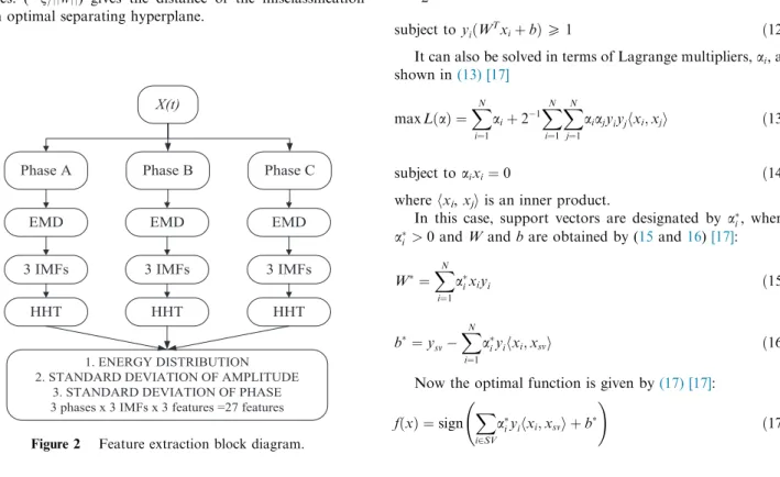
Thus three features for each IMF among three IMFs con-stitute a data set of nine features for each phase. The entire process of feature extraction stage is shown inFig. 2.

2.4. Support Vector Machines (SVMs)

The SVM evolved from theory to implementation and results, whereas neural networks follow heuristic path from applica-tions to experiments. Also, SVMs are less prone to over fitting problems and give sparse solution when compared to neural and do not depend on input space dimensionality. Many of the classification problems have been addressed by SVM.

Classification using SVM basically involves training and testing data which is composed of many instances. In training set, each instance consists of two attributes (features in this case) and a target value called class label (usually 1 or1). The aim of this classifier is to create a model which can suc-cessfully predict the class label of unknown data or test data instance which consists of only attributes. However, most of the SVM algorithms can classify between only two classes thus making it a two class problem[16–18]i.e., separating the set of training data i.e., (x1,y1), (x2,y2),. . ., (xn,yn), wherexi2Rnis feature vector andyi2{1, +1} class vector. The two classes are separated by a hyperplane as shown inFig. 3. The dashed lines indicate the margin and the points on the margin are called support vectors. Optimal separating hyperplane is at a distance of (b/||w||) from origin.nis a variable that measures the amount of misclassification in case of non-separable classes. (n/||w||) gives the distance of the misclassification from optimal separating hyperplane.

Hyperplane,g(x) which accurately separates the data into its corresponding classes as in[17]is given by(9)

WT_x

iþb¼0 ð9Þ

whereWis a vector with real values andbis a constant. Their values should be derived in such that the unknown data are classified accurately. This is possible by maximizing the separa-tion margin between the classes which is defined as shown in (10) [17].

m¼ 2

kWk ð10Þ

For maximizingm,Wshould be minimized. According to [17], for a given set of linearly separable data, this can be for-mulated as quadratic optimization problem as shown in(11). min1

2kWk

2 _ð

11Þ subject toyiðWTxiþbÞP1 ð12Þ It can also be solved in terms of Lagrange multipliers,ai, as shown in(13) [17] maxLðaÞ ¼X N i¼1 aiþ21X N i¼1 XN j¼1 aiajyiyjhxi;xji ð13Þ subject toaixi¼0 ð14Þ

wherehxi,xjiis an inner product.

In this case, support vectors are designated by a_i, where a

i >0 andWandbare obtained by (15and16)[17]:

W¼X N i¼1 a ixiyi ð15Þ b¼ysv XN i¼1 a iyihxi;xsvi ð16Þ Now the optimal function is given by(17) [17]:

fðxÞ ¼sign X i2SV a iyihxi;xsvi þb ! ð17Þ

Phase A Phase B Phase C

HHT

X(t)

1. ENERGY DISTRIBUTION 2. STANDARD DEVIATION OF AMPLITUDE

3. STANDARD DEVIATION OF PHASE 3 phases x 3 IMFs x 3 features =27 features

EMD EMD EMD

3 IMFs 3 IMFs 3 IMFs

HHT HHT

Figure 2 Feature extraction block diagram.

In case if data cannot be separated linearly then (W*_,b*₎ does not exist. Then the input data should be mapped first fromn-dimensional space (Rn) to higher dimensional feature space (Fm)[17]:

/:Rn _{! F}m_x

i ! /ðxiÞ ð18Þ

Then another functionfis used to map the data from fea-ture space to decision space (Y2)[17]:

f:Fm _{! Y}2_/ðx

iÞ ! fð/ðxiÞÞ ð19Þ An SVM classifier separating two nonlinearly separable classes is shown inFig. 4.

Usually kernel functions are used for mapping nonlinearly separable data into higher dimensional feature space. Thus Eq. (17)can be modified as follows[17]:

fðxÞ ¼sign X i2SV a iyikðxi;xsvÞ þb ! ð20Þ where kðxi;xsvÞis kernel function. Equation of k for Radial Basis Function (RBF) is given as in(21) [17]:

kðx;yÞ ¼exp jjxyjj

2

2r2

!

ð21Þ Various kernel functions are available, while Gaussian RBF kernel is proved to be reliable kernel functions for this purpose [15]. In this paper Gaussian RBF kernel is used.

3. System under study

A simple three phase power system is modeled in SIMULINK environment. It includes three lines, 500 km, 200 km and 150 km with impedance values per km (R, X, C) for zero sequence is (0.3064, 0.9654, 7.751106) and for positive

sequence is (0.01273, 0.2026, 12.74106) respectively. The power system network is shown inFig. 5. Fault is applied on 500 km line at various locations. Three parameters of the selected system are varied: (1) Load Angle (10°, 20° and 30°), (2) Fault location (varied from 10 km to 100 km in inter-vals of 20 km from source) and (3) Fault Resistance (0.1 and 100 ohms). Thus a total of 450 cases are taken into study, out of which 400 cases are used for training SVM and 50 cases are used for testing SVM.

4. Combined three SVM model

In this paper, a multiple SVM model is employed which con-stitutes three SVMs.SVM-A,SVM-BandSVM-Care trained to detect fault in A,B andCphases respectively. In testing phase each SVM classifies the fault as class 1 if the fault is detected in corresponding phase; otherwise, it is classified as class1. Fault is determined using the combination of results from all the three SVMs according to the logic sequences shown inTable 1.

Special case corresponds to a situation where the model cannot classify between double line to ground faults and three phase faults. In such case the following procedure is followed for classifying between ABG, BCG, CAG and three phase

faults.

1. Check each phase for voltage lag or voltage rise using peak values of voltages in each phase using instantaneous ampli-tude values.

2. Drop in instantaneous amplitude during a particular period (fault period) in all the three phases indicates three phase faults.

3. Drop in two phases and rise in third phase indicate double line to ground fault.

X X X X X X X X X O O O O O O O O O Φ (X ) Φ (X ) Φ (X ) Φ (X ) Φ (X ) Φ (X ) Φ (O ) Φ (O ) Φ (O ) Φ (O ) Φ (O ) Φ (O ) Φ (O ) Φ (O )

INPUT SPACE _{FEATURE SPACE}

Φ (X ) Φ (X ) Φ (X ) Φ (X ) Φ (X ) Φ (X ) Φ (O ) Φ (O ) Φ (O ) Φ (O ) Φ (O ) Φ (O ) Φ (O ) Φ (O ) FEATURE SPACE

C1

C2

R

F

F

Y

The overall Multiple SVM model can be represented as shown inFig. 6.

5. Results and discussion

All the data for training and testing phase are acquired by simulating the sample model (Fig. 5) using SimPowerSystems toolbox in SIMULINK environment (R2009b). The proposed algorithm is implemented using Matlab 7 software on a Windows 7 operating system with Intel core i3-870 system

G

π

π

π

π

G

Figure 5 Power system network.

Table 1 Multiple SVM logic for fault classification.

SVM ‘A’ SVM ‘B’ SVM ‘C’ Fault type

1 1 1 AG 1 1 1 BG 1 1 1 CG 1 1 1 AB 1 1 1 BC 1 1 1 CA 1 1 1 Special case INPUT FEATURES SVM - A SVM - A SVM - B SVM - C LOGIC SEQUENCER AG BG CG ABG BCG CAG ABCG AB BC CA Verify Instantaneous amplitude

Figure 6 Implementation of multiple SVM model.

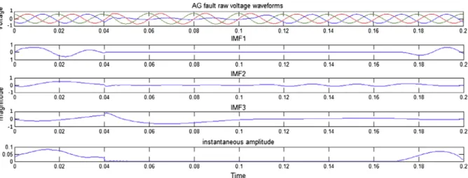
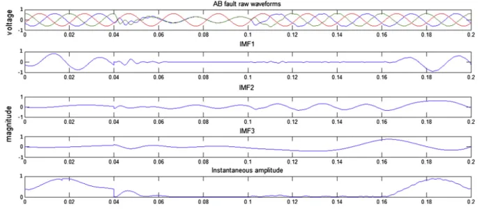
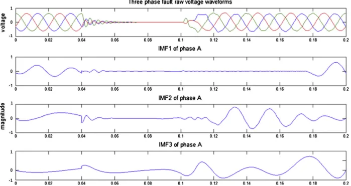
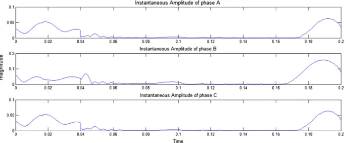
and the methodology takes the computational time of 1.92 s for classifying a typical fault. This computation time varies from case to case analysis of the chosen test system. Voltage waveforms for one single line to ground fault case (AG), one line to line fault case (AB), one double line to ground (ABG) and one three phase fault condition are shown inFigs. 7–10 along with IMF1–3 and instantaneous amplitude for phase-A. For ABG fault and ABCG fault, instantaneous ampli-tudes of IMF1 of all the three phases are shown separately inFigs. 11 and 12. For ABG fault (Fig. 11) the instantaneous

amplitude for phase-A and B is decreased throughout the fault situation, while for phase-C, instantaneous amplitude is raised once fault is occurred. For three phase faults (Fig. 12), in all the three phases instantaneous amplitude is diminished upon occurrence of fault. This property is used for classifying between double line to ground fault and three phase faults under special condition shown inTable 1. All the three SVMs are trained rigorously using the data obtained by varying parameters of the sample mode. SVM toolbox of MATLAB software is used for this purpose. A combination Figure 8 AB fault: voltage waveforms, IMF1–3 and instantaneous amplitude of phase A.

of Coupled Simulated Annealing (CSA) and a standard sim-plex method is used for optimizing the following two param-eters of SVM: (1) Regularization parameter, c which determines the trade-off between the training error, minimiza-tion and smoothness, and (2) squared bandwidth,r2_{. Initially}

CSA is used to calculate good starting values and they are

passed to the simplex method in order to fine tune the result. The optimized values of c and bandwidth are shown in Table 2. The results show that out of 50 cases chosen ran-domly among 450 for validating the proposed methodology, the classifier identifies accurately with efficiency of 95% and above.

Figure 10 ABC fault: voltage waveforms, IMF1–3 and instantaneous amplitude of phase A.

6. Conclusion

In this paper, a hybrid algorithm to classify the power system fault is proposed. The proposed technique uses multiple SVM model with features extracted using Empirical Mode Decom-position and Hilbert Huang Transform algorithms. Classifica-tion is done among ten fault cases with rigorous training and testing phases. Accuracy and feasibility of the proposed methodology are demonstrated by results obtained. The main contribution of the proposed algorithm is the possibility of its application to any transmission line, no matter the line config-uration, with no need for re-training at different load values, voltage levels and fault resistances. In this paper, a simple power system network is trained and tested for evaluating the algorithm. From the results it has identified that the algorithm is producing good results on fault classification. However, the algorithm functionality does not depend on number of buses or complexity of the network. Hence the proposed algorithm is expected to work for any number of buses if training is done accordingly. The classification efficiency does not depend upon fault resistance, location of fault or the load value.

Acknowledgment

The authors would like to thank School of Electrical Engineer-ing, VIT University for providing facilities and support to execute this project.

References

[1] Aravena JL, Chowdhury FN. A new approach to fast fault detection in power systems. Int Conf Intell Syst Appl Power Syst, Florida, USA; 1996. p. 328–32.

[2] Youssef OAS. Online applications of wavelet transforms to power system relaying. IEEE Trans Power Delivery 2003;18(4): 1158–65.

[3] Youssef OAS. ‘Online applications of wavelet transforms to power system relaying – Part II’. IEEE Power Eng Soc Gen Meet 2007:1–7.

[4] Manjula M, Sarma AVRS, Naga Lakshmi GV. Wavelet trans-form for classification of voltage sag causes using probabilistic neural network. Int J Electr Eng 2011;4(3):299–309.

[5] Youssef OAS. Combined fuzzy-logic wavelet-based fault classifi-cation technique for power system relaying. IEEE Trans Power Delivery 2004;19(2):582–9.

[6] Youssef OAS. An optimized fault classification technique based on support-vector-machines. IEEE/PES Power Syst Conf Expos 2009:1–8.

[7] Sevakula RK, Verma NK. Wavelet transforms for fault detection using svm in power systems. IEEE Int Conf Power Electron Drives Energy Syst, Bengaluru, India; December 2012. p. 1–6.

[8] Livani H, Evrenosoglu CY. A fault classification method in power systems using DWT and SVM classifier. IEEE/PES Trans Distrib Conf Expo 2012:1–5.

[9] Shukla S, Mishra S, Singh B. Empirical-mode decomposition with hilbert transform for power-quality assessment. IEEE Trans Power Delivery 2009;24:2159–65.

Figure 12 Instantaneous amplitude of IMF1 of phase A–C for three phase faults.

Table 2 SVM classifiers parameters and performance.

SVM RBF kernel parameters No. of testing cases No. of cases classified accurately Efficiency of classifier (%) Overall efficiency SVM-A c= 23 r2 = 0.4 50 48 96 SVM-B c= 26 r2_{= 0.4} 50 49 98 95.33% SVM-C _c= 23 r2_{= 0.4} 50 46 92

[10]Manjula M, Sarma AVRS, Mishra S. Empirical mode decompo-sition based probabilistic neural network for faults classification. Int Conf Power Energy Syst 2011:1–5.

[11]Manjula M, Sarma AVRS, Mishra S. Detection and classification of voltage sag causes based on empirical mode decomposition. Annual IEEE India Conf (INDICON) 2011:1–5.

[12]Huang NE, Wu MLC, Long SR, Shen SSP, Qu W, Gloersen P, Fan KL. A confidence limit for the empirical mode decomposition and Hilbert spectral 18 analysis. Proc R Soc A: Math Phys Eng Sci 2003;459:2317–45.

[13]Huang E, Shen Z, Long SR. The empirical mode decomposition and the Hilbert spectrum for nonlinear and non-stationary time series analysis. Proc R Soc Lond 1998;454:903–95.

[14] Barnhart B. The Hilbert–Huang transform: theory, applications, development. Ph.D. dissertation, University of Iowa; 2011. [15]Guo Y, Li C, Li Y, Gao S. Research on the power system fault

classification based on HHT and SVM using wide-area informa-tion. Sci Res Energy Power Eng 2013;5:138–42.

[16] Gunn SR. Support vector machines for classification and regres-sion. Ph.D. dissertation, University of Southampton, UK; 1997. [17]Cristianini N, Shawe-Taylor J. An introduction to support vector

machines and other kernel-based learning methods. Cambridge University Press; 2000.

[18]Zhang Q, Yang YQ. Research of the kernel function of support vector machine. Electr Power Sci Eng 2012;28(5):42–5.

N. Ramesh Babureceived his bachelor’s degree in Electrical and Electronics Engineering in Bharathiar University, India, and received his master’s degree in Applied Electronics from Anna University, India. Also he obtained his Ph.D. degree from VIT University, India. He has published several technical papers in national and international conferences and international journals. His current research includes Wind Speed Forecast, Optimal Control of Wind Energy Conversion System, Solar Energy and Soft Computing techniques applied to Electrical Engineering.

B. Jagan Mohanis a graduate in Bachelor of Technology (Electrical and Electronics Engi-neering) from VIT University, Vellore, India. He published papers on speech recognition. His area of interest is Signal Processing and Robotics.