HAL Id: hal-02472760
https://hal.archives-ouvertes.fr/hal-02472760
Submitted on 10 Feb 2020
HAL
is a multi-disciplinary open access
archive for the deposit and dissemination of
sci-entific research documents, whether they are
pub-lished or not. The documents may come from
teaching and research institutions in France or
abroad, or from public or private research centers.
L’archive ouverte pluridisciplinaire
HAL
, est
destinée au dépôt et à la diffusion de documents
scientifiques de niveau recherche, publiés ou non,
émanant des établissements d’enseignement et de
recherche français ou étrangers, des laboratoires
publics ou privés.
Crowd Behavior Characterization for Scene Tracking
Gianni Franchi, Emanuel Aldea, Séverine Dubuisson, Isabelle Bloch
To cite this version:
Gianni Franchi, Emanuel Aldea, Séverine Dubuisson, Isabelle Bloch. Crowd Behavior Characterization
for Scene Tracking. 2019 16th IEEE International Conference on Advanced Video and Signal Based
Surveillance (AVSS), Sep 2019, Taipei, Taiwan. pp.1-8, �10.1109/AVSS.2019.8909893�. �hal-02472760�
Crowd Behavior Characterization for Scene Tracking
Gianni Franchi,
Emanuel Aldea
S´everine Dubuisson
Isabelle Bloch
SATIE, Universit´e Paris-Sud
CNRS, LIS
LTCI, T´el´ecom Paris
Universit´e Paris-Saclay
Aix Marseille University
Institut polytechnique de Paris
Orsay, France
Marseille, France
Paris, France
Abstract
In this work, we perform an in-depth analysis of the spe-cific difficulties a crowded scene dataset raises for tracking algorithms. Starting from the standard characteristics de-picting the crowd and their limitations, we introduce six en-tropy measures related to the motion patterns and to the ap-pearance variability of the individuals forming the crowd, and one appearance measure based on Principal Compo-nent Analysis. The proposed measures are discussed on syn-thetic configurations and on multiple real datasets. These criteria are able to characterize the crowd behavior at a more detailed level and may be helpful for evaluating the tracking difficulty of different datasets. The results are in agreement with the perceived difficulty of the scenes.
1. Introduction
The difficulty of performing scene tracking (i.e., track-ing collectively the individuals present in the scene) relates directly to the complexity of the motion patterns and to the variability in terms of visual appearance of the pedestrians. In practice, these variables are influenced by more com-plex factors which are difficult to infer and model, such as the pedestrian objectives or their socio-cultural background. These general assumptions justify that the tracking diffi-culty depends on the crowd behavior.
We therefore propose to study the behavior of a crowd. This is a hard point because crowds are composed of a mul-titude of pedestrians who may engage in trajectories ex-hibiting a wide range of dynamics. Indeed each person has his/her own purpose, however, the movement of people is self-organized often without anyone deciding consciously. Furthermore, this is a compromise between individual be-haviors and collective behavior that we want to characterize in a compact representation. In fact, a given dataset made up of people with rather independent behaviors may be harder Contact: [email protected], [email protected], [email protected], [email protected]
to track than one composed of collective movement. This last type of crowd makes it possible to propose general rules that an algorithm of tracking must follow. This is used in many articles (e.g. [1, 3]).
To study this relationship between collective and isolated movement, we propose to study the disorder of the crowd. Indeed, measuring crowd disorder hints to the chaotic as-pect of its dynamics, or otherwise stated to what extent the pedestrian movement is collective.
In this article, we propose to measure two types of dis-order. There exists a high number of works related to this task [7, 14], but in our work we will specifically focus on formulations based on the Shannon entropy. The first type of disorder we intend to evaluate is related to the actual mo-tion, and it relates a collective motion to pedestrians walk-ing with the same velocity and in the same direction. Our contribution regarding this term is that we conduct a lo-cal evaluation, and prove the interest of inferring lolo-cally, in contrast to several works [2, 10, 11, 12, 13]. For the second type of disorder, we propose to study to what extent people look the same, hence we speak of disorder of appearance. This disorder can allow one to understand whether people look locally the same or not. Based on this information, we can compare crowds in terms of fundamentally different, but highly relevant measures of homogeneity and charac-terize more accurately the degree of difficulty faced by a tracker.
2. Related work
Our work is related to a large body of criteria, measures or techniques which aim to interpret the behavior of the crowd. We can broadly divide these works into two fam-ilies, namely microscopic and macroscopic measures.
In the following, we will describe a series of microscopic characteristics used to describe a crowd. One of the simplest criteria is the number of persons, which is however highly relevant in our setting since a crowd featuring a high num-ber of persons might be harder to follow for reasons related to computational cost. Another important microscopic
acteristic is the spatial layout of the tracks, which depict the trajectories of all individuals forming the crowd.
In order to study a crowd at microscopic level, one must locate all the instances present in the data set. On the other hand, by accounting for the spatial distribution of instances, one can describe the density of the crowd. We define the density at timetand at a positionxthe number of people in the neighbourhood ofx. This characterization is a macro-scopic measure.
In practice, different algorithms [5, 8] are now able to estimate the density of a crowd without deriving it from mi-croscopic measures.
Macroscopic characterization may be performed by identifying groups of persons. Groups are clusters that can evolve during time since some individuals may switch groups. The definition of a group is not really clear since it relates further to the notion of interaction between indi-viduals. This interaction between two people can be char-acterized for example by the fact that they walk in the same direction, that they are close to each other, or they both in-teract with a third object. Hence the definition of groups depends highly on the context, but finding groups may as-sist in describing a crowd.
Starting from a set of measures considered as relevant, one may analyze the crowd behavior. In [7], five families of movement have been established, i.e. blocking, lane, bottle-neck, ring/arch, fountainhead. As shown in this article, the behavior establishes a global movement of the crowd. As in [7], many approaches resort to characterizing the crowd based on local representations, similarly to fluid dynamics. Hence they evaluate the motion of trajectories, and, based on the divergence of these flows, they classify the crowd. This classification is interesting, however it does not pro-vide any real measure of collective movement of the crowd. An improvement with respect to this characterization is the measure of collectiveness proposed in [14]. It measures to what degree the behavior of each individual of a crowd acts as a union in collective motion. To measure the col-lective movement path similarities is integrated across the
K-nearest neighbor graph. This approach seems to work well on various crowd systems, but under the assumption that motion collectiveness derives mainly from orientation, hence the influence of the relative speed of movement of each person with respect to their immediate neighbors is ig-nored.
Another idea developed in several works [2, 10, 11, 12, 13] is to evaluate the global entropy of a crowd. Entropy can be used to evaluate how much a crowd movement is choice-less or not. However, the main limitation of these techniques is that they study the movement globally. Let us consider two settings, each time with a crowd consisting of two groups of people heading towards each other, with each group exhibiting a very coherent movement. Let us assume
that the difference between the two situations is that in the configuration S1 the two groups intersect, while in S2 the two groups are very far from each other. It seems logical to consider that S2 is more ordered than S1. However, a global entropy will not underline this difference, thus it seems im-portant to rely on a local entropy formulation. This is what we will propose in the next section.
3. Proposed entropy-based local crowd
charac-terization
A crowd can be seen as multiple sets of Markov chains since it is commonly admitted that the state of the person at timet+ 1depends on his/her state at timet. However, these sets of tracks depend on each other since they might interact. Hence, at a given time t the position of track i
might depend on all or some other tracks developing at time
t. Understanding and accounting for this interaction is key to characterizing the crowd behavior. To understand this synergy, three major questions can be raised: 1)Is the crowd homogeneous? 2)Is the crowd isotropic? and 3)Does the crowd walk in a homogeneous way?
3.1. Notations and definitions
A video can be seen as a set ofnframes{I(t), t= 1...n}
whereI(t)is a 2D image, i.e. a scalar valued matrix. We
noteo(it) = (xi(t), w, h)the objectiof the framet; in our case, the objects are the pedestrian heads,x(it)denotes the 2D coordinates of objectiinI(t),handware respectively
the height and the width of the bounding box of the object, which are assumed constant for all the persons. Each frame
thasNtobjects.
Let us denote byFi(t)the(w×h)-size crop in the image whose top right corner isx(it)and containing the bounding box of each objecto(it). We consider that this crop is the intrinsic feature space describing the object i at frame t. Any alternative descriptor extraction may be used with no loss of generality, but we avoid in the following to tie our analysis to the behaviour of a specific descriptor.
We define a crowd to be homogeneous in appearance or in velocity if all the people of the crowd have the same ap-pearance or the same velocity. We define a crowd to be isotropic if the moving direction of the people present in the crowd is the same.
3.2. Characterizing the motion of the crowd
The question about the isotropic properties of the crowd motion can be answered via the collectiveness [14]. Eval-uating the isotropy of the crowd consists in measuring whether people have a consistent trajectory and how much their trajectories are consistent with each other. There are different ways to address this matter. One can be interested
in studying the isotropy at small scales, thus focusing on local isotropy, or alternatively one might want to study the global isotropy. We show on a toy example in the experi-mental section that, depending on what we look at, the local study brings additional relevant information.
Regarding the movement of the crowd, the isotropy is important but one can also be interested in studying whether pedestrians walk at the same velocity or not. This study is related to the homogeneity of the displacement. This aspect is crucial since it might create traffic jams.
We propose to study these two questions at the same time thanks to a local/global entropy. At a given time,t, we de-fine a graphG(t) = (O(t),E(t)), where the vertex setO(t)
is the set of persons present at frame t,E(t) is the set of
edges connecting the vertices. We consider that the graph is not weighted, or alternatively edges have a weight of 1 for linked nodes and 0 otherwise. One node is connected to its
Knearest neighbors. For a given node we explore different ways to calculate its nearest neighbors. The first proposition is to calculate its nearest neighbors based on the Euclidean distance between the position of the persons. Hence the local entropy based on theseKnearest neighbors will rep-resent the entropy of pedestrians being close spatially This entropy will illustrate the spatial disorder in the crowd. We will denote this entropy as the spatial local entropy.
Another solution is to identify theK nearest neighbors according to their direction using the cosine distance de-fined as: D(x(it),x(jt)) = 1− x (t) i .x (t) j ||x(it)||.||x(jt)||
where·is the dot product.Based on this distance the nearest neighbors of a pedestrian are considered as the pedestrians the most coherent in terms of direction. This entropy fo-cuses mostly on the displacement of a crowd since by con-sidering people that have almost the same orientation we evaluate their entropy. We denote this entropy asthe col-lective local entropy.
Finally, one might be interested in the entropy of people that are spatially close to each other and go in the same di-rection. In order to evaluate this local entropy, we calculate the matrix of the Euclidean distances between all vertices at a frametand we normalize it by dividing all its components by the maximum distance. We do the same for the matrix of cosine distances. The final distance is the weighted sum of these two normalized distances (commensurability is en-sured by the normalization). In our experiments, we chose equal weights (i.e. 0.5) for each distance. We denote this entropy asthe group local entropy.
Thanks to these different distances, we have differentK
nearest neighbors and thus different measures of local en-tropy. Now, we describe how to calculate the local entropy based on theKnearest neighbors. We estimate the crowd
displacement entropy based on Shannon’s entropy [6]. We estimate for each vertex of the graph a probability density function of displacement. Inspired by the work in [13], we consider two random variables. A first variable X repre-sents the orientation of the displacement. Hence, at a given time we count how many people are moving in this direc-tion. The second random variableY represents the distance of the displacement of the pedestrians. Similarly to [13] we estimate the joint probability functionP(X, Y)of these two random variables, then based on the probability density function we estimate the Shannon entropy:
H(X, Y) =−X l,p
P(X=xl, Y =yp) lnP(X=xl, Y =yp)
However, in contrast to [13], we estimate a local joint prob-ability function PK,i(X, Y)for each node i of the graph,
which is the joint probability function on theKneighbors of the objecto(it). Hence, this probability function depends on the neighborhood sizeK, and on the vertexi. Thus we define our local entropy as:
Hloc(X, Y) = − 1 Nt X i,l,p PK,i(X =xl, Y =yp) lnPK,i(X=xl, Y =yp)
This entropy formula is not a proper entropy since this is a mean of all entropies. But it synthesizes all the information provided by the whole set of local entropies.
3.3. Characterizing the appearance of the crowd
To study the homogeneity of the people in the crowd we propose to use a similar local entropy but with a new ran-dom variable, denoted byZ. For simplicity of comparison we convert the images to gray-scale images, and divide the scale uniformly in a fixed number of bins. The random vari-able is a scalar which measures the probability that a given gray level belongs to one of the bins. Based on this distri-bution we evaluate the local entropy as follows:
Hloc(Z) =− 1
Nt
X
i,p
Pk,i(Z=zp) lnPk,i(Z =zp) (1)
The use of the differentK nearest neighbors proposed in the previous section is the key point of our local en-tropy that we define in Equation 1. The different locality brings different information about people and their appear-ance. For example, the spatial local entropy provides infor-mation about the appearance of closed persons. The col-lective local entropy allows us to check whether the people who walk in the same direction look the same. The group local entropy gives information on whether people on the same group present similar clothes and look the same.
Finally to study the homogeneity of the appearance we propose to perform a Principal Component Analysis (PCA) on the matrix gathering the crop of every people, and then reduce the number of meaningful dimensions. Let us con-sider a set of vectors{v(it)} ∈ Rw×h,1 ≤ i ≤ Nt. We
consider that we have a vector for each person, which rep-resents all the information taken from a crop around the per-son. Hence the vectorvi(t)represents the cropFi(t)that has been reshaped to a vector. The goal of the classical PCA is to reduce the dimension of this vector space ofRw×h ,
to vector spaceRd,where d w×hthanks to a
projec-tion. The matrix of the data is a matrix that represents a concatenation of all the vectors v(it) where each row in
Rw×hcorresponds to a vectorized crop (i.e.Fi(t)), and each
column inRNtcorresponds to a concatenation of the values of each crop at the same location. In our case, we want to reduceNtto have the minimal number of person that can
represent the dataset at timet, hence find a mapping
{gj(t)}wj=1×h∈RNt−→ {g˜j(t)} w×h j=1 ∈R
nt (2)
withgj(t)a column of the matrix of data withj∈[1, w×h], andntNt. This is achieved using PCA, by keeping only
thentcomponents corresponding to the largest eigenvalues,
that best explain the variance of the data. Finally the last proposed measures is:
MPCA= nt
Nt
(3)
4. Evaluation and applications
For all experiments, we set the random variableX rep-resenting the orientation of the displacement to lie within four bins equally spaced in[0,2π[. The random variableZ
representing the greyscale values that will take a pixel of the crop of a person lies within 10 bins equally spaced in
[0,255[. Finally, we quantify the random variableY, repre-senting the distance of displacement, into five bins, namely
[0,1[,[1,3[,[3,6[,[6,9[,[9,∞[. The first bin is intended to count the number of people who do not move. The second one accounts for the people who move slowly. The third one provides us the number of people who move with moderate velocity and the two last bins correspond to the fast moving people.
4.1. Single scale analysis of synthetic datasets
In this first experiment we compare the discriminative power of the different entropy definitions proposed in this paper. For that, we simulated several examples of crowd motions: each crowd has a different behavior. We computed on these crowds the global entropy, local entropies and the collectiveness measure proposed in [14]. The probability
distribution used in the entropy calculation contains only the displacement information.
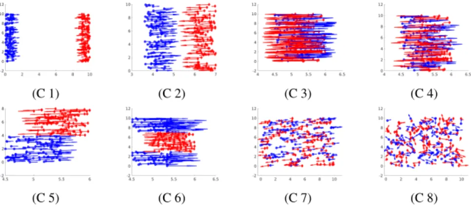
Each simulated configuration contains 200 people (100 red and 100 blue). Their positions were randomly chosen depending on different scenarios, described below. For all simulations, speeds of displacement are uniformly drawn over [0,6] pixels, except for C3 for which it is set to 1 pixel. For all the simulations except C8, the directions of movement of the people in blue are drawn uniformly over
[0◦,15◦], and those of the people in red over[180◦,195◦]. The simulations are described below and Figure 1 shows, for each simulation, the pedestrians (diamonds or circles), and their displacements (each arrow representing the ampli-tudes and directions of this displacement).
C1: the blue pedestrians move on the left and the red ones on the right. These two groups are far apart.
C2: similar to C1 but the two groups are closer to each other.
C3: similar to C1 but the two groups intersect, and the ve-locity of the pedestrians in the crowd is constant and set to1.
C4: similar to C3 except that the velocity of the pedestrians in the crowd is not constant.
C5: similar to C4 but the two groups organized themselves in lines. This corresponds to a lane formation. C6: similar to C5, but in this case a central lane is flanked
by two opposing lanes.
C7: similar to C4 but the two groups of pedestrians are more distant. In some sense, we spread the pedestrian locations in a wider area.
C8: total chaos case, where the initial locations are drawn uniformly on the[0,10]pixels, and the next ones fol-low a Gaussian random walk.
These synthetic examples are used to determine which of the measures is best suited to describe each crowd case. Results are given in Table 1. For these experiments we used
K= 15(number of nearest neighbours).
Results in Table 1 allow us to draw some preliminary conclusions. First, the global entropy used in most of the articles to measure the disorder of crowds is not precise enough since it provides a similar value for all scenarios, and thus we cannot actually distinguish the behavior of the different crowds.
The collectiveness does not characterize the speed of movement of a crowd. Thus a crowd that moves in one direction but that contains pedestrians moving at different speeds is considered as containing no disorder, which can be problematic in some cases. Thus the characterization of the
(C 1) (C 2) (C 3) (C 4)
(C 5) (C 6) (C 7) (C 8)
Figure 1: Visualization of the simulated crowd (scenario cases are described in Section 4.1).
C 1 C 2 C 3 C 4 C 5 C 6 C 7 C 8 Collecti-venes 0.99 0.98 0.10 0.10 0.94 0.87 0.01 0.00 Global entropy 1.54 1.55 0.69 1.63 1.55 1.56 1.58 1.93 Spatial local entropy 0.77 0.80 0.61 1.40 0.85 0.94 1.40 1.69 Collective local entropy 0.82 0.77 0.00 0.90 0.73 0.87 0.97 1.52 Group local entropy 0.77 0.80 0.05 0.87 0.82 0.83 0.88 1.44
Table 1: Values of different measures of crowd behavior depending on the scenario.
crowd is not complete. Moreover, the collectiveness does not correctly describe situations C7 and C8 which seem to have the same level of disorder while one is totally chaotic and the other has a disordered collective movement (that can be interpreted as a relative organization).
The three local entropies that we propose better charac-terize the crowds because they measure additional informa-tion that can help to analyze a crowd. For example, if we compare C7 and C4, we can see that they present the same statistical information. The major difference between these two simulations is that people in crowd C7 are closer to each other than the ones in crowd C4. However, the results of the collectiveness seem to differentiate them. Our entropy measures are more consistent with this observation. If we compare C1 and C2 we see that the collective local entropy is smaller for C2 because people in this crowd have a more coherent movement. But the people in C2 are locally more disordered as it may be seen from the spatial local entropy value. In addition, C1 and C2 have a smaller disorder than any other simulation regardless of the measurement. If we compare C5 and C6, we find that C6 is more chaotic
what-Figure 2: Visualization of the simulated multi-group crowd.
ever the measure. If we compare C3 and C4, we notice that the measure of collectiveness does not reflect the disorder in C3 which is different from that of C4.
4.2. Multi-scale analysis of synthetic datasets
In this example, we have simulated 4 groups, illustrated in Figure 2. The blue group contains 20 people with posi-tions randomly drawn in[0,2]×[0,8]. Their displacement direction is to the right, uniformly drawn over[0◦,15◦]. The red group contains 120 persons with positions randomly chosen in [13,15]×[6,15]. Their direction is to the left drawn uniformly in[180◦,195◦]. The green group contains 50 people with positions randomly chosen in[4,12]×[3,5]. Their direction is upwards, drawn uniformly in[90◦,105◦]. The black group contains 10 people with positions ran-domly chosen in[3,5]×[13,15]. Their direction is down-wards, drawn uniformly in[270◦,285◦].
In this experiment we want to study the multi-scale be-havior of local entropies. Results are given in the Ta-ble 2, depending on the considered neighborhood sizeK. They show that there are discontinuity breaks for K = 10,20and120, which are related to the group dimensions. Thus one can infer that the multi-scale analysis makes it possible to highlight notions of groups on crowds, hence to
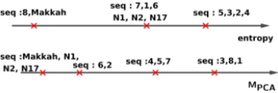
Figure 3: Motion entropy on the real sequences (Sec-tion 4.3).
discover more complex structures.
4.3. Real datasets
We also have evaluated the different measures on the UCF dataset [3] which is a real-world crowd tracking dataset, composed of 8 sequences. Sequence 1 contains crowds with a linear movement in opposite directions, sim-ilarly to our C6 simulation. Sequence 2 is a dense crowd with mainly two major directions. Sequences 3, 4 and 6 show crowds during sport events, where all the people seems to go in one direction. Sequence 5 is also a crowd sport event but in arch movement. Sequences 7 and 8 are lane movements where a large group of people follows one major direction and a small group follows a different direc-tion. In addition to these sequences, we propose to study a dataset acquired in Makkah. This dataset shows people during Islamic pilgrimage. One of the major difficulties is that all pilgrims have a similar appearance. We have also annotated 3 sequences1which corresponds to sequence 1, 2 and 17 of [4], we refers to them as N1 N2 and N17. This implies that they are barely distinguishable for the human eye at the scale of the videos. Details on the sequences are provided in Table 3.
Table 4 presents the motion entropy results. One can see that Sequences 3, 4 and 6 have a small local entropy, due to the global straight (aligned) direction of motion: most of the people have the same motion. Sequence 5 has high global and spatial local entropies, but low collective and group lo-cal entropies. This is because this dataset is composed of people running a marathon on a circular road hence it is possible to find groups of people having the same motion. Sequences 1 and 7 seem to have more motion disorder than the other sequences. This is because there is no real motion structure in these sequences. In Figure 3 we have drawn the order of motion entropy based on global and local analysis, the axis representing thus an increasing difficulty of track-ing with respect to the pedestrian motion.
Tables 5 and 6 provide the appearance entropy and the proportion of the principal component, in order to summa-rize the appearance of the people. The principal compo-nent measures to what extent crops of people look the same, while the entropy measures the entropy of color on crops of
1http://hebergement.u-psud.fr/emi/MOHICANS/ Crowd_annotation_Dataset.zip.
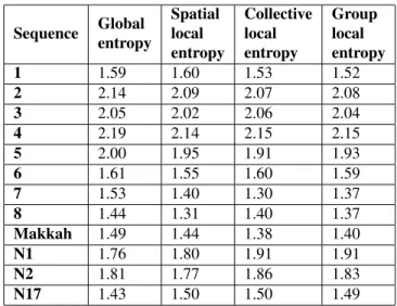
Figure 4: Appearance entropy and PCA on the sequences of Section 4.3.
people. Hence they do not necessarily measure the same point.
We can see from Table 5 that Sequences 8 and Makkah have a lower entropy than the other sequences since most of the people on these sequences have similar appearance with white or black clothing. In Sequences 1, 6, 7 N1, N2 and N17, the colors are quite uniformly distributed, and finally come sequences 2, 3, 5 and 4.
Regarding the reduction property of the PCA results in Table 6, we can see that compression is more efficient for the sequences Makkah, N1, N2 and N17, followed by the sequences 6, 2, 4, 5, 7. Then, come the sequences 3, 8, 1. The easier the compression, the harder it is to track regard-ing the appearance.
In Figure 4 we have drawn the order of the appearance entropy based on global and local analysis and also based on theMPCA. Please note in contrast to Figure 3, this
rep-resents in decreasing order of difficulty of tracking. One can see that the behavior ofMPCA and entropy are
not the same. Indeed, the entropy checks whether the colors are the same in all the crops while the PCA checks how much principal components can synthesize all the data set. This confirms that PCA highlights structural information.
Our intuition was that the difficulty of a database is proportional to the entropy of motion and inversely pro-portional to the appearance entropy. Hence to prove this point we apply two tracking algorithms that have state-of-the-art results (deep flow algorithm [9] and NMC [3]), and we present in Table 7 their tracking accuracy results. The tracking accuracy is defined in [3]. Despite the fact that a simple (ideally linear) correspondence between the en-tropy values and the tracking accuracy is difficult to estab-lish, the results may be interpreted in order to further adapt the tracking strategy to the challenges raised by a specific dataset. Inevitably, different algorithms may have com-pletely contrasting approaches in exploiting appearance and motion information. With respect to the considered algo-rithm, we can note that sequence 7 and Makkah, that exhibit the worst tracking accuracy, have a higher motion entropy and a lower appearance entropy. By contrast, sequences 2 and 4, that have the best tracking accuracy, have less motion entropy and a higher appearance related entropy. Thanks to these local entropies we have access to an entropy value for
K 10 20 30 40 50 60 70 80 90 100 110 120 130 140 150
Spatial local entropy 1.09 1.20 1.24 1.26 1.28 1.29 1.30 1.33 1.34 1.34 1.35 1.36 1.43 1.48 1.52
Collective local entropy 1.02 1.17 1.25 1.26 1.26 1.29 1.30 1.30 1.29 1.29 1.27 1.27 1.36 1.50 1.57
Group local entropy 1.09 1.18 1.22 1.22 1.24 1.25 1.24 1.28 1.28 1.28 1.27 1.28 1.38 1.49 1.54
Table 2: Results of the local entropy with different sizes of neighborhood.
Sequence # people # frames
max density average displa-cement 1 152 840 12.3 0.5 2 235 134 3.0 0.8 3 175 144 4.9 2.8 4 747 492 16.5 4.4 5 147 464 7.4 1.3 6 600 333 14.7 1.1 7 73 494 2.3 1.1 8 58 126 2.0 1.2 Makkah 620 50 5.0 3.8 N1 200 14 3.1 0.5 N2 153 14 3.2 0.6 N17 173 50 3.9 0.5
Table 3: Quantitative and microscopic measures performed on real crowd datasets. # people: number of people, # frames: number of frames, max density: density max over all the frames, and average displacement: average of all the displacements (in pixels) of all the people in the crowd.
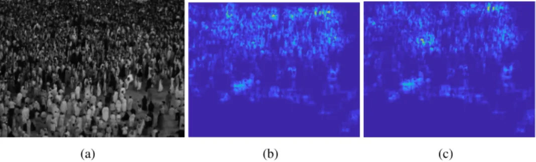
each person of the crowd. This provides a hint on not nor-mal behaviors. Figure 5 summarizes the local entropies for Makkah database, high values correspond to high entropies.
Sequence Global entropy Spatial local entropy Collective local entropy Group local entropy 1 2.01 1.82 1.48 1.49 2 1.96 1.57 1.25 1.23 3 1.34 1.10 0.76 0.77 4 0.66 0.36 0.49 0.45 5 1.82 1.20 0.99 0.98 6 1.40 1.10 0.80 0.82 7 2.13 1.58 1.51 1.39 8 1.92 1.50 1.40 1.25 Makkah 1.88 1.21 1.21 1.18 N1 1.70 1.53 1.43 1.40 N2 1.78 1.68 1.68 1.40 N17 1.62 1.54 1.43 1.43
Table 4: Motion entropy of real crowd datasets.
Sequence Global entropy Spatial local entropy Collective local entropy Group local entropy 1 1.59 1.60 1.53 1.52 2 2.14 2.09 2.07 2.08 3 2.05 2.02 2.06 2.04 4 2.19 2.14 2.15 2.15 5 2.00 1.95 1.91 1.93 6 1.61 1.55 1.60 1.59 7 1.53 1.40 1.30 1.37 8 1.44 1.31 1.40 1.37 Makkah 1.49 1.44 1.38 1.40 N1 1.76 1.80 1.91 1.91 N2 1.81 1.77 1.86 1.83 N17 1.43 1.50 1.50 1.49
Table 5: Appearance entropy of real crowd datasets.
Sequence MPCA 1 0.184 2 0.033 3 0.101 4 0.060 5 0.075 6 0.040 7 0.082 8 0.103 Makkah 0.016 N1 0.010 N2 0.010 N17 0.013
Table 6: Measure of the proportion of principal compo-nents needed to summarize the appearance of the real crowd datasets.
(a) (b) (c)
Figure 5: (a) One frame of Makkah sequence. (b) The appearance local spatial entropy of (a). (c) The motion local spatial entropy of (a). Sequence Tracking accuracy flow tracking [9] Tracking accuracy NMC [3] 1 60% 80% 2 100% 100% 3 88% 92% 4 96% 94% 5 59% 77% 6 84% 94% 7 65% 67% 8 89% 92% Makkah 39% 78% N1 99% 97% N2 95% 94% N17 94% 94%
Table 7: Performance of state-of-the-art tracking algorithms on real crowd datasets. We use as measure of performance the tracking accuracy defined in [3]. The second column contains results of tracking of deep flow algorithm [9]. The third column contains results of NMC [3] tracking algo-rithm.
5. Conclusions
This work aims to formalize from a broader perspective the degree of difficulty raised by a crowd dataset toward tracking tasks. The proposed measures highlight in a com-pact way the motion as well as the appearance variability of the data, in the form of local and global entropy measures. These entropies can help us to understand the homogeneity and the isotropy of the crowd, which are essential indicators for explaining its behaviour. A real application of these lo-cal entropies would be to use the information they provide to understand the abnormal behavior of a crowd.
In future work, we intend to underline more extensively the relationship between these measures of entropy and the performance of different tracking strategies.
References
[1] S. Ali and M. Shah. Floor fields for tracking in high density crowd scenes. InEuropean Conference on Computer Vision, pages 1–14. Springer, 2008.
[2] S. Behera, D. P. Dogra, and P. P. Roy. Characterization of dense crowd using gibbs entropy. InProceedings of 2nd In-ternational Conference on Computer Vision & Image Pro-cessing, pages 289–300. Springer, 2018.
[3] H. Idrees, N. Warner, and M. Shah. Tracking in dense crowds using prominence and neighborhood motion concurrence. Image and Vision Computing, 32(1):14–26, 2014.
[4] M. K. Lim, V. J. Kok, C. C. Loy, and C. S. Chan. Crowd saliency detection via global similarity structure. In 2014 22nd International Conference on Pattern Recognition, pages 3957–3962. IEEE, 2014.
[5] V. Ranjan, H. Le, and M. Hoai. Iterative crowd counting. In ECCV, pages 270–285, 2018.
[6] C. E. Shannon. A mathematical theory of communication. Bell system technical journal, 27(3):379–423, 1948. [7] B. Solmaz, B. E. Moore, and M. Shah. Identifying
behav-iors in crowd scenes using stability analysis for dynamical systems.TPAMI, 34(10):2064–2070, 2012.
[8] J. Vandoni, E. Aldea, and S. L. H´egarat-Mascle. Evaluating crowd density estimators via their uncertainty bounds. In ICIP. IEEE, 2019.
[9] P. Weinzaepfel, J. Revaud, Z. Harchaoui, and C. Schmid. Deepflow: Large displacement optical flow with deep match-ing. InProceedings of the IEEE International Conference on Computer Vision, pages 1385–1392, 2013.
[10] G. S. Ying Zhao, Mengqi Yuan and T. Chen. Entropyand dynamics analysis ofcrowd motions phase transition. 2015. [11] X. Zhang, Z. He, et al. Crowd panic state detection using
entropy of the distribution of enthalpy.Physica A: Statistical Mechanics and its Applications, 2019.
[12] Y. Zhao, M. Yuan, G. Su, and T. Chen. Crowd macro state detection using entropy model. Physica A: Statistical Me-chanics and its Applications, 431:84–93, 2015.
[13] Y. Zhao, M. Yuan, G. Su, and T. Chen. Crowd security de-tection based on entropy model. InISCRAM, 2015. [14] B. Zhou, X. Tang, and X. Wang. Measuring crowd
collec-tiveness. InProceedings of the IEEE conference on computer vision and pattern recognition, pages 3049–3056, 2013.