Kent Academic Repository
Full text document (pdf)
Copyright & reuse
Content in the Kent Academic Repository is made available for research purposes. Unless otherwise stated all content is protected by copyright and in the absence of an open licence (eg Creative Commons), permissions for further reuse of content should be sought from the publisher, author or other copyright holder.
Versions of research
The version in the Kent Academic Repository may differ from the final published version.
Users are advised to check http://kar.kent.ac.uk for the status of the paper. Users should always cite the published version of record.
Enquiries
For any further enquiries regarding the licence status of this document, please contact: [email protected]
If you believe this document infringes copyright then please contact the KAR admin team with the take-down information provided at http://kar.kent.ac.uk/contact.html
Citation for published version
Guerre, Emmanuel (2019) Quantile regression methods for first-price auctions. arXiv . (Submitted)
DOI
Link to record in KAR
https://kar.kent.ac.uk/77789/
Document Version
Quantile regression methods for first-price auctions
Nathalie Gimenes
Department of Economics
PUC-Rio
Brazil
[email protected]
Emmanuel Guerre
School of Economics
University of Kent
United Kingdom
[email protected]
September 2019
Abstract
The paper proposes a sieve quantile regression approach for first-price auctions with symmetric risk-neutral bidders under the independent private value paradigm. It is first shown that a private value quantile regression model generates a quantile regression for the bids. The private value quantile regression can be easily estimated from the bid quantile regression and its derivative with respect to the quantile level. A new local polynomial technique is proposed to estimate the latter over the whole quantile level interval. Plug in estimation of functionals is also considered, as needed for the expected revenue or the case of CRRA risk-averse bidders, which is amenable to our framework. A quantile regression analysis to USFS timber is found more appropriate than the homogenized bid methodology and illustrates the contribution of each explanatory variables to the private value distribution.
JEL: C14, L70
Keywords: First-price auction; independent private value; dimension reduction; quantile regression; local polynomial estimation; sieve estimation; boundary correction.
A previous version of this paper has been circulated under the title ”Quantile regression methods for first-price auction:a signal approach”. The authors acknowledge useful discussions and comments from Xiao-hong Chen, Valentina Corradi, Yanqin Fan, Phil Haile, Xavier d’Haultfoeuille, Vadim Marmer, Isabelle Per-rigne, Martin Pesendorfer and Quang Vuong, and the audience of many conferences and seminars. Nathalie Gimenes also thanks Ying Fan and Ginger Jin for encouragements. All remaining errors are our responsi-bility. Both authors would like to thank the School of Economics and Finance, Queen Mary University of London, for generous funding.
1
Introduction
Various quantile approaches have been recently proposed for the Econometrics of Auctions. Haile, Hong and Shum (2003, HHS hereafter) have used monotonicity of bidding strategy to build a quantile test of the independent private value null hypothesis. Milgrom (2001, Theorem 4.7) reformulates the identification relation of Guerre, Perrigne and Vuong (2000, GPV afterwards) using quantile function. The risk aversion identification result of Guerre, Perrigne and Vuong (2009, GPV09 hereafter) heavily relies on the bid quantile function in first-price auctions. Zincenko (2018) develops a corresponding nonparametric estimation method. Liu and Luo (2017) and Liu and Vuong (2018) have respectively developed quantile based test for the null of exogenous participation and monotonicity of the bidding strategy. Other authors have considered quantile based estimation of the private value distribution. Gimenes (2017) has implemented a quantile regression approach for ascending auction. See also Menzel and Morganti (2013) who proposed an order statistics approach. For first-price auction, Marmer and Shneyerov (2012) has proposed a quantile-based estimator of the private value probability density function (pdf), which is an alternative to the two step GPV method. Guerre and Sabbah (2012) have noted that the private value quantile function can be estimated using a one step procedure from the estimation of the bid quantile function and its first derivative. Enache and Florens (2015) have developed an inverse problem approach. The two step method of GPV focuses on the private value pdf estimation, which is quite hard to estimate. Estimating pdf is useful for descriptive purposes and for computation of important moments, such as the expected revenue. But the latter can also be achieved using quantile functions, as moments are easily computed integrating it. As noted in Milgrom (2001) in the independent private value setting, the value function of a bidder observing a uniform signal is nothing else than the private value quantile function, so that a quantile approach is especially relevant in auction settings. Nonparametric density estimation is notoriously affected by the curse of dimensionality, and parsimonious models addressing this issue for density are less rich than for quantile functions, where both single index modelling, as already used in an auction framework by Marmer, Shneyerov and Xu (2013b), and additive
specification are available. A simpler specification is the homogenized bid model of HHS, which postulates a regression model with iid residuals for the private value. As shown in our empirical application and in Gimenes (2017) for ascending auctions, it may fail to capture nonlinear dependence of the private value to auction covariate. In addition, it still involves a GPV step that may not perform well in small samples.
The present paper develops a quantile regression methodology for first-price auctions, which includes parsimonious but flexible models suitable for moderate samples. The param-eter of interest is the private value conditional quantile function given some auction specific covariates, which can be estimated faster than the conditional pdf. A key aspect of our ap-proach is that the bid conditional quantile function is a linear functional of the private value one. It follows that the popular quantile regression model of Koenker and Bassett (1978) can play a central role in our methodology, as it enjoys an important stability property: a private value quantile regression model generates a bid quantile regression model. The private value quantile function is a linear combination of the bid quantile function and its first derivative with respect to the quantile level, a simple identification method which is the basis of our estimation procedure. This also applies to the linear sieve quantile regression of Belloni, Chernozhukov, Chetverikov and Fern´andez-Val (2017). Following Horowitz and Lee (2005), the latter can be tailored to additive quantile models, which can be better estimated that saturated sieve models. Higher order covariate interactions can also be considered, giving a class of flexible models which can be tailored to each specific datasets.
An important challenge is raised by the estimation of the bid quantile derivative with respect to the quantile level α. This was considered by Guerre and Sabbah (2012) and the references therein. We propose instead a new local polynomial approach which applies to quantile levels and aims to jointly estimate the bid quantile function and its derivatives. An unexpected feature is that it performs well for extreme quantile levels, producing consistent estimators for α = 0 and 1. The latter upper quantile levels are particularly important for auctions as private values of winners are expected to be in the top of the distribution. Recent work focusing on boundary issues are Aryal, Gabrielli and Vuong (2016) in a semiparametric
framework and Hickman and Hubbard (2015). Our theoretical results include a Central Limit Theorem for the private value quantile estimator which holds for extreme quantiles and a bias variance decomposition for its Integrated Mean Squared Error (IMSE). The latter allows in particular for bandwidth choice based on a pilot quantile model.
A second family of parameters of interest consists in integral functionals of the bid quan-tile function and its quanquan-tile level first derivatives. A first example is the parameter of Constant Relative Risk Aversion (CRRA) utility functions. CRRA risk aversion preserves indeed the quantile linearity features which are important for our quantile regression method-ology. The risk aversion parameter can be estimated using bidder variations as in GPV09 but also combining first-price and ascending auction as in Lu and Perrigne (2008). A second example is the expected revenue, which falls in such family as it is a functional of the private value quantile function (Gimenes, 2017), see also Li, Perrigne and Vuong (2003). A third ex-ample covers the conditional private value cumulative distribution function and pdf. Indeed the rearrangement formula of Chernozhukov, Fern´andez-Val and Galichon (2010) expresses the cdf as an integral functional of the private value quantile function. Differentiating a smooth version of this functional proposed in Dette and Volgushev (2008) gives a pdf esti-mator which fits in our framework and differs from Marmer and Shneyerov (2012). These distribution estimators are useful for dimension reduction purpose.
Our theoretical results are illustrated with a simulation experiment and an application to USFS first price auctions. A preliminary quantile regression analysis of the bid quantile function suggests that the homogenized bid technique should not be applied here because the quantile regression slopes are not constant. The private value quantile regression slope functions reveal the impact of the covariate, and how strongly bidders in the top of the distribution can differ from the bottom. CRRA risk-aversion estimation using the approaches of GPV09 and Lu and Perrigne (2008) is also considered. The rest of the paper is organized as follows. The next section introduces our quantile identification approach and the functionals of interest. Section 3 introduces our local polynomial estimation framework. Section 4 groups our main theoretical results for the private value quantile functions and its functionals. Our
simulation results are in Section 5 and the application can be found in Section 6. Section 7 summarizes the estimation strategy and the empirical application findings, and describes some possible extensions. All the proofs are gathered in six Online Appendices.
2
First price auction and quantile specification
A single and indivisible object with some characteristicx∈RD is auctioned to I ≥2 buyers.
The potential number of biddersI and x are known to the bidders and the econometrician. Bids are sealed so that a bidder does not know others’ bid when forming his own bid. The object is sold to the highest bidder who pays his bid Bi to the seller. Under the symmetric
IPV paradigm, each potential bidder is assumed to have a private value Vi, i = 1, . . . , I
for the auctioned object. A buyer knows his private value but not the private value of the other bidders, but the joint distribution of theVi is common knowledge. The private values
are independently and identically drawn from a distribution given (x, I) with a compactly supported cdf F (·|x, I), or equivalently with conditional quantile function
V (α|x, I) =F−1(α|x, I), α in [0,1].
The private value quantile function is the first parameter of interest of the present paper, to be estimated from bids Bi from the symmetric Bayesian Nash equilibrium. Section 2.4
below considers a second set of parameters of interest derived from V (·|·,·) such as the cdf
F (·|·,·) or the associated pdf f(·|·,·).
2.1
Private value quantile identification
It is well-known that the bidder i private value rank
has a uniform distribution over [0,1] and is independent ofx and I. It also follows from the IPV paradigm that the private value ranks Ai = 1, . . . , I are independent. The dependence
between the private value Vi and the auction covariates x and I is therefore fully captured
by the non separable quantile representation
Vi =V (Ai|x, I), Ai iid
∼ U[0,1] ⊥(x, I).
Following Milgrom and Weber (1982) or Milgrom (2001), V (·|x, I) can also be viewed as a
valuation function, the private value rank Ai being the associated signal. In what follows,
G(·|x, I) andg(·|x, I) stand for respectively the bid conditional cdf and pdf.
Maskin and Riley (1984) have shown that Bayesian Nash Equilibrium bidsBi =σ(Vi;x, I)
of symmetric risk averse or risk neutral bidders must strictly and continuously increase with the private values under the IPV paradigm. It follows that Bi = B(Ai|x, i) where
B(·;x, i) =σ(F(·|x, I) ;x, I) can be viewed as a bidding strategy depending upon the rank
Ai. If F (·|x, I) is also strictly increasing, so is B(·|x, I) and since Ai is uniform it holds
G(b|x, I) = P[B(Ai|x, I)≤b|x, I] =P
Ai ≤B−1(b|x, I)|x, I
=B−1(b|x, I) showing that the bidding strategy B(·|x, I) is also the bid quantile function.
A standard best response argument will show how to identify the private value quantile function V (·|x, I) from B(·|x, I). Suppose bidderi signal Ai is equal to α, but that her bid
is a suboptimal B(a|x, I), all other bidders bidding B(Aj|x, I). Then the probability that
bidder iwins the auction is
P B(a|x, I)> max 1≤j6=i≤IB(Aj|x, I) Ai =α, x, I =P a > max 1≤j6=i≤IAj Ai =α, x, I =aI−1 (2.1) because the Aj’s are independent U[0,1] independent of xand I. It follows that the expected
is a best-response bidding strategy, the optimal bid of a bidder with signal α is B(α|x, I), that is α= arg max a (V (α|x, I)−B(a|x, I))aI−1 .
As B(·|x, I) is continuously differentiable, it follows that
∂ ∂a (V (α|x, I)−B(a|x, I))aI−1 a=α = 0 (2.2)
or equivalently dαd αI−1B(α|x, I) = (I −1)αI−2V (α|x, I). Solving with the initial condi-tion B(0|x, I) = V (0|x, I) and rearranging the equation above gives Proposition 1, which is the cornerstone of our estimation method. From now on B(1)(α|x, I) = dαdB(α|x, I).
Proposition 1 Consider a given (x, I), I ≥2, for which α ∈ [0,1]7→ V (α|x, I) is contin-uously differentiable with a derivative V(1)(·|x, I)>0. Suppose the bids are drawn from the
symmetric differential Bayesian Nash equilibrium. Then,
i. The conditional equilibrium quantile function B(·|x, I) of the I iid optimal bids Bi
satisfies B(α|x, I) = I−1 αI−1 Z α 0 aI−2V (a|x, I)da. (2.3)
ii. The bid quantile functionB(α|x, I)is continuously differentiable over[0,1]and it holds V (α|x, I) =B(α|x, I) + αB
(1)(α|x, I)
I−1 . (2.4)
A key feature is the linearity of the private value to bid quantile function mapping (2.3), which implies that a private value quantile linear model is mapped into a similar bid linear model, as detailed below for the well known quantile regression. Proposition 1-(ii) shows that the private value quantile function is identified from the bid quantile function and its
derivative, as noted in Guerre and Sabbah (2012). It is a quantile version of the identification strategy of GPV, based on the computation of the private value from the bid1
Vi =Bi+ 1 I−1 G(Bi|x, I) g(Bi|x, I) .
Versions of (2.4) withB(1)(α|x, I) changed into 1/g(B(α|x, I)|x, I) can be found in Milgrom (2001, Theorem 4.7), Liu and Luo (2014), Enache and Florens (2015), Liu and Vuong (2016) and Luo and Wan (2016) and, under risk aversion, in GPV09 and Campo, Guerre, Perrigne and Vuong (2011). As developed in Section 2.4 below, Proposition 1 can be extended to the case of symmetric risk-averse bidders with a CRRA utility function.
2.2
Private value quantile regression and homogenized bids
Private value quantile regression. The linearity of (2.3) with respect to the private value quantile function has remained unnoticed with very few exceptions, although it has important model stability implications useful for practical implementation. Consider for instance a private value quantile given by the quantile regression specification
V (α|x, I) =γ0(α|I) +x0γ1(α|I) = [1, x0]γ(α|I) . (2.5)
Proposition 1-(i) implies that the conditional bid quantile function satisfies,
B(α|x, I) = [1, x0]β(α|I) with β(α|I) = I −1
αI−1
Z α 0
tI−2γ(t|I)dt, (2.6) showingB(α|x, I) belongs to the quantile regression specification. It follows from (2.4) that
γ(α|I) = β(α|I) + αβ
(1)(α|I)
I−1 , (2.7)
1This can be recovered from (2.4) taking α = A
i as Vi = V (Ai|x, I), Bi = B(Ai|x, I) implying that Ai=G(Ai|x, I) andB(1)(Ai|x, I) = 1/g(B(Ai|x, I)|x, I) = 1/g(Bi|x, I).
so that γ(α|I) can easily be estimated from an estimation of β(α|I) and β(1)(α|I). It then follows that the quantile regression specification is stable, i.e. a quantile regression specification for the private value is equivalent to a quantile regression specification for the bid. Hence testing the correct specification of a bid quantile regression model is equivalent to test the correct specification of a private value quantile specification. The expressions (2.6) and (2.7) show that significance testing can be done through bid quantile regression as γj(·|I) = 0 is equivalent to βj(·|I) = 0, or more generally e0γ(·|I) = c is equivalent to
e0β(·|I) = cfor any conformable e and c.
Bid homogenization and quantile regression. HHS have noted that a translation of the private values results in a similar translation of the bids, an invariance property that they use in their bid homogenization technique. The latter can be interpreted as the use of a regression model for the private values,Vi =γ0+x0γ1+vi with an error term vi independent
of x, as also proposed by Rezende (2008). This amounts to assume that the slope function
γ1(·|I) in (2.5) does not depend upon the quantile level. The regression model of HHS and
Rezende (2008) is indeed equivalent to the quantile regression specification
V (α|x) = γ0+x0γ1+v(α)
where v(α) is the quantile function of vi. Since αII−−11
Rα
0 a
I−2da = 1, it follows that the
associated bid quantile function is, by (2.3)
B(α|x, I) = γ0+x0γ1+b(α|I), where b(α|I) =
I−1
αI−1
Z α
0
aI−2v(a)da.
This gives the bid regression model
Bi =β0(I) +x0γ1+bi, β0(I) =γ0+E[b(Ai|I)]
where the regression error term bi = b(Ai|I)−E[b(Ai|I)] is centered and independent of
and the distribution of vi can be estimated applying the GPV two step method to the
homogenized bids, which are the residuals Bi−x0bγ1.
However this approach requests independence between the regression error term vi and
the covariatex, an assumption which may be too restrictive in practice as found by Gimenes (2017) and the application below. When γ1(·) is not a constant, regressing B(α|x, I) on
[1, x] givesBi =β0(I) +x0β1(I) +b(Ai|x, I) with a slope coefficient satisfying
β1(I) = Z 1 0 I−1 αI−1 Z α 0 aI−2γ1(a)da dα = Z 1 0 γ1(α)dα− Z 1 0 Z α 0 a α I−1 γ(1)1 (a)da dα
and a residual termb(Ai|x, I) =v(Ai) +x0AI−I−11
i
RAi 0 a
I−2γ
1(a)da−β1(I) which now depends
upon x, so that the homogenized bid approach does not apply. Using variation of I can be useful to detect such a situation because observing variation of β1(I) implies that γ1(·)
is not a constant. In particular, If the entries of γ1(1)(·) are nonnegative, the entries of
β1(I) must increase with I. Similar features hold for centered bids Bi −E[Bi|I] when
the homogenized bid regression is replaced by a nonparametric regression: the regression functionE[Bi−E[Bi|I]|x, I] should not depend uponI ifVi =m(X) +vi, as for the single
index regression specification considered in Paarsch and Hong (2006).
2.3
Linear nonparametric quantile specification
Flexible interactive specifications. The private value quantile regression model (2.5) assumes linearity of the private value quantile function with respect to the covariatex. This may be too strong and can be relaxed using a quantile nonparametric additive specification, which was considered in Horowitz and Lee (2005). Recall thatx= (x1, . . . , xD) and consider
the additive quantile function
V (α|x, I) =
D
X
j=1
where each functionsVj(α;xj, I) is specific to the entryxj. Since such quantile specifications
are obtained by summing some univariate functions, the effective dimension involved in the nonparametric dimension of this model is 1 because it can be estimated with the same rate than a nonparametric model with a unique covariate as shown in Horowitz and Lee (2005). This parsimonious model can be generalized following Andrews and Whang (1990) to allow for more covariate interactions. This leads to the additive interactive quantile specification with DM interactions V (α|x, I) = DM X δ=1 X 1≤j1<···<jδ≤d Vj1...jδ(α;xj1, . . . xjδ, I) (2.9)
where each functions Vj1...jδ(α;xj1, . . . xjδ, I) can now depend upon δ entries of x with
δ ≤ DM ≤ D. Setting DM equal to the dimension D of the covariate gives the general
quantile specification. As seen from Andrews and Whang (1990) for the regression case, such specification can be estimated with the same rate than a function of DM variables, so
that DM can be viewed as the effective dimension of this model.
The stability property in Proposition 1-(i) ensures that a private value quantile specifi-cation withDM interaction will generate a bid quantile specification with the same number
of interactions: if (2.9) holds, then the bid quantile function satisfies
B(α|x, I) = DM X δ=1 X 1≤j1<···<jδ≤d Bj1...jδ(α;xj1, . . . xjδ, I)
and the private values components of the specification can be recovered using Proposition 1-(ii).
Sieve interactive specification. The interactive quantile specification (2.9) can be esti-mated using a sieve expansion, as in Horowitz and Lee (2005) or Andrews and Whang (1990). Consider a sieve{Pk(x),1≤k≤K} is a family of functionsPk(·) =PkK(·) allowing for at
such that for all α V (α|x, I) = lim K→∞ K X k=1 γk(α|I)Pk(x). (2.10)
The expression (2.10) can be viewed as a sieve extension of the quantile regression, a sieve quantile regression. It follows from Proposition 1-(i,ii) that, provided the limit in (2.10) holds uniformly with respect toα,
B(α|x, I) = lim K→∞ K X k=1 βk(α|I)Pk(x), βk(α|I) = I−1 αI−1 Z α 0 tI−2γk(t|I)dt, (2.11) V (α|x, I) = lim K→∞ K X k=1 βk(α|I) + αβk(1)(α|I) I−1 ! Pk(x). (2.12)
Hence estimating the private value sieve quantile regression can proceed from estimating the coefficients of the bid sieve quantile regression in (2.11) and their first derivatives.
2.4
Risk aversion, expected payoff and other functionals
Many auction parameters of interest can be written using the private value quantile functions, or equivalently the bid quantile function and its quantile derivative by (2.4). We focus here on the conditional and unconditional integral functionals
θ(x) = Z 1 0 F α, x, B(α|x, I), B(1)(α|x, I) ;I ∈ I dα, θ= Z X θ(x)dx (2.13) whereF(α, x, b0I, b1I;I ∈ I) is a real valued continuous function. Three illustrative examples
are as follows.
Example 1: CRRA risk aversion. For symmetric risk averse bidders with a concave utility function, the best response condition (2.2) becomes
∂ ∂a U(V (α|x, I)−B(a|x, I))aI−1 a=α = 0.
Rearranging as in GPV09 yields thatV (α|x, I) = B(α|x, I)+λ−1αB(1)(α|x,I)
I−1
whereλ(·) =
U(·)/U0(·). For risk averse bidders with a CRRA utility function U(t) =tθ, arguing as for Proposition 1 shows V (α|x, I) =B(α|x, I) +θαB (1)(α|x, I) I−1 , (2.14) B(α|x, I) = 1 αI−θ1 Z α 0 tI−θ1−1V (t|x, I)dt.
These two formulas show that the stability implications of Proposition 1 for linear private value and bid quantile functions are preserved under CRRA. Assuming as in GPV09 that the number of bidders is exogenous, i.e V (α|x, I) = V (α|x) for all I, gives, for any pair
I0 6=I1 θ = θn θd = R X h R1 0 (B(α|x, I1)−B(α|x, I0)) αB(1)(α|x,I 0) I0−1 − αB(1)(α|x,I 1) I1−1 dα i dx R X R1 0 αB(1)(α|x,I 0) I0−1 − αB(1)(α|x,I 1) I1−1 2 dα dx , (2.15)
a formula which shows that the CRRA risk aversion can be easily identified from first-price auction. Following Lu and Perrigne (2008), the risk-aversion parameter θ can also be iden-tified combining ascending and first-price auctions data. As seen from Gimenes (2017), the private value quantile function Vasc(α|x, I) can be easily estimated from ascending auctions.
Equating Vasc(α|x, I) to V (α|x, I) in (2.14) gives that θ satisfies
θ= R X h R1 0 (Vasc(α|x, I)−B(α|x, I)) αB(1)(α|x,I) I−1 dα i dx R X R1 0 αB(1)(α|x,I) I−1 2 dα dx . (2.16)
Example 2: Expected revenue. Suppose that the seller decides to reject bids lower than a reserve price R and let αR = αR(x, I) be the associated screening level, i.e. αR =
F (R|x, I). For CRRA bidders, the first price auction seller’s expected revenue is2 ERθ(αR|x, I) = θ·I·V (αR|x, I) (I −1) (θ−1) +θα I−1 θ R 1−α(I−1) θ−1 θ +1 R + I(I−1) (I−1) (θ−1) +θ Z 1 αR tI−θ1−1 1−t(I−1)θ−θ1+1 V (t|x, I)dt. (2.17) This expression includes an integral item
θ(x;αR) = Z 1 αR tI−θ1−1 1−t(I−1)θ−θ1+1 V (t|x, I)dt
which can be estimated by plugging in a risk aversion estimatorθband an estimatorVb(α|x, I) of the private value quantile function, or estimators of the bid quantile function and its derivative by (2.4).3
Example 3: Private value distribution Chernozhukov et al. (2010) have used the rearrangement formula to invert a monotonic function. In our case, the conditional private value cdf satisfies
F (v|x, I) =E[I[V (A|x, I)≤v]|x, I] = Z 1
0
I[V (α|x, I)≤v]dα, A∼ U[0,1].
Dette and Volgushev (2008) have considered a smoothed versionIη(·) of the indicator
func-tion
Fη(v|x, I) =
Z 1
0
Iη[v−V (α|x, I)]dα
2It is assumed for the sake of brevity that the seller value for the good is 0.The expected revenue formula
for the general case follows from Gimenes (2017).
3Under risk-neutrality, integrating by parts gives that
Z 1 αR B(1)(α|x, I)αI−1(1−α)dα=B(αR|x, I)αIR−1(1−αR)− Z 1 αR B(α|x, I)αI−1(I−1−Iα)dα,
where Iη(t) =
Rt/η
−∞k(u)du, k(·) being a kernel function and η a bandwidth parameter.
Differentiating Fη(v|x, I) gives fη(v|x, I) = 1 η Z 1 0 k v−V (α|x, I) η dα
which converges to the private value pdf whenηgoes to 0. Note thatFη(v|x, I) andfη(v|x, I)
can be estimated by plugging in an estimator Vb(α|x, I) of V (α|x, I). The resulting cdf and pdf estimator are expected to inherit of the dimension reduction property of this procedure. As the private value estimator Vb(α|x, I) proposed in the next section is consistent over the whole [0,1], no trimming is needed. This contrasts with the GPV pdf estimator.
3
Augmented quantile regression estimation
Proposition 1 suggests to base the estimation of the private value quantile function on es-timations of B(α|x, I) and of its derivative B(1)(α|x, I) with respect to α. While there is an important literature on the estimation of a conditional quantile function, estimating the first derivative of a quantile function has received much less attention. The augmented
methodology applies local polynomial expansion with respect to α for joint estimation of
B(α|x, I) and B(1)(α|x, I). Sieve methods can be used for the covariate. To ensure com-parability with the literature, we assume that the private value quantile function V (α|x, I) has s+ 1 continuous derivatives with respect to α. As seen from (2.3), this implies that the bid quantile function B(α|x, I) hass+ 2 continuous derivatives with respect to α >0. This justifies the order s+ 1 for the local polynomial estimator considered here.
3.1
Definition of the estimators
The no covariate case. Consider L iid first-price auctions (I`, x`, Bi`, i= 1, . . . , I`). To
B(α|I). Let ρα(·) be the check function,
ρα(q) = q(α−I(q ≤0)),
I(·) being the indicator function, I(q≤0) = 1 for q ≤ 0 and 0 otherwise. It is well known
that,
B(α|I) = arg min
q E[I(I` =I)ρα(Bi`−q)], α∈(0,1) .
Estimating the derivativeB(1)(α|I) can be done by introducing local variation of the quantile
level in the vicinity ofα. LetK(·)≥0 be a kernel function with support [−1,1] and h=hL
be a positive bandwidth parameter going to 0 with the sample size. Then it follows that
{B(a|I), a∈[α−h, α+h]∩[0,1]} = arg min q(a) Z 1 0 E[I(I` =I)ρa(Bi`−q(a))] 1 hK a−α h da, (3.1) where the minimization is performed over the set of functions q(a) which are continuous on [α−h, α+h]∩[0,1]. Instead of a minimization over such a rich set of functions, we consider minimization over a set of polynomial functions. Indeed, a good polynomial approximation of B(a|I) over [α−h, α+h] is given by the Taylor expansion
B(a|I) = B(α|I) +B(1)(α|I) (a−α) +· · ·+ B
(s+1)(α|I) (a−α)s+1 (s+ 1)! +O h s+2 . Letb = (β0, . . . , βs+1) 0
be the generic coefficients of such a polynomial function and
π(a) = 1, a,a 2 2 . . . , as+1 (s+ 1)! 0 .
The sample version of the objective function (3.1) restricted to polynomial functions is b R(b;α, I) = 1 LI L X `=1 I(I` =I) I` X i=1 Z 1 0 ρa Bi`−π(a−α) 0 b1 hK a−α h da = 1 LI L X `=1 I(I` =I) I` X i=1 Z 1−hα −α h ρα+ht Bi`−π(ht) 0 bK(t)dt.
Theaugmented quantile estimator isbb(α|I) = arg minbRb(b;α, I),βb0(α|I) andβb1(α|I) being estimators of B(α|I) and its first derivative B(1)(α|I), respectively.4 The estimator of the private value quantile is5
b
V (α|I) =βb0(α|I) +
αβb1(α|I)
I−1 .
Augmented quantile regression. A first extension of this procedure is the augmented quantile regression estimator, AQR hereafter, which considers the private quantile regression specification
V (α|x, I) = [1, x0]γ(α|I).
4When the private value distribution does not depend uponI, the bid quantile functionsB(·|I) are such
that the derivatives
∂j ∂αj B(α|I) +αB (1)(α|I) I−1 = 1 + j I−1 B(j)(α|I) +αB (j+1)(α|I) I−1
do not depend upon I as they are equal to V(j)(α|I) = V(j)(α), j = 0, . . . , s+ 1. These constraints
can be used to estimate V(α) using the parameters γ = (γ0, . . . γs) , δ = (δ2, . . . , δI) where γj is for V(j)(α) and δI for the derivatives B(s+1)(α|I), I = 2, . . . , I and bI(γ, δ) = [b0,I, . . . , bs,I, δI]0 with bs,I = 1 + I−s1 −1 γs−Iα−1δI
and thebj,I’s are computed recursively using
bj,I = 1 + j I−1 −1 γj− α I−1bj+1,I ,j = 0, . . . , s.
The estimator ofV (α) isbγ0where
b γ,bδ = arg minγ,δP I I=2Rb(bI(γ, δ) ;α, I).
5Although not considered here, the augmented quantile estimation procedure can be used to estimate the
p.d.f. f(v|I) of the private value using f(v|I) = 1/V(1)[F(v|I)|I]. An estimator for F(·|I) is Vb−1(·|I). Set Vb(1)(α|I) = βb1(α|I) +αβb2(α|I)/(I−1) and fb(v|I) = 1/Vb(1)
h b
F(v|I)|Ii. This p.d.f. estimator can account for covariates by using the AQR and ASQR procedures introduced below.
In the second extension, the augmented sieve quantile regression (ASQR), the private value quantile function V (α|x, I) is equal to P (x)0γ(α|I) up to an approximation error, where
P (x) stacks the sieve functions Pk(x), k = 1, . . . , K. The AQR and ASQR approaches can
be grouped setting P (x) = [1, x0]0 for the AQR.
The bid quantile function satisfies B(α|x, I) = P (x)0β(α|I) by (2.6) with γ(α|I) =
β(α|I) + αβ(1)(α|I)/(I −1) by (2.7), up to an approximation error in the ASQR case.
Define now the parameter
b=β00, β10, . . . , βs0+1
where all theβj have the same dimensionD+ 1 and
P (x, t) =π(t)⊗P(x)
which is such that the Taylor expansion ofB(α|x, I) writes, in the AQR case,
B(α+ht|x, I) =P (x, ht)0b(α|I) +O hs+2
where b(α|I) stacks β(α|I) and its successive derivatives β(1)(α|I), . . . , β(s+1)(α|I). The objective function of the estimation procedure becomes
b R(b;α, I) = 1 LI L X `=1 I(I` =I) I` X i=1 Z 1 0 ρa Bi`−P (x`, a−α) 0 b 1 hK a−α h da = 1 LI L X `=1 I(I` =I) I` X i=1 Z 1−hα −α h ρα+ht Bi`−P(x`, ht) 0 bK(t)da (3.2) which accounts for the covariatex`. The estimation ofb(α|I) isbb(α|I) = arg minbRb(b;α, I) and the private value quantile regression estimator is
b
V (α|x, I) = P (x)0γb(α|I) withγb(α|I) =βb0(α|I) +
αβb1(α|I)
I−1 .
The bid quantile function and its derivatives can be estimated usingBb(α|x, I) = P (x)
0
b
andBb(1)(α|x, I) =P (x)
0
b
β1(α|I). The rearrangement method of Chernozhukov et al. (2010)
can be used to obtain increasing quantile estimators.
3.2
Boundary estimation
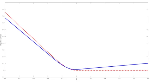
Bassett and Koenker (1982) report that standard quantile regression estimators are not defined for the extreme quantile levels α = 0 or α = 1 or even nearby. The augmented procedures proposed here are better behaved for extreme quantiles because the objective function Rb(·;α, I) averages the check function ρa(·) for quantile levels a in [α−h, α+h]∩ [0,1]. For instance, if α = 1 and h ≤1, Rb(b; 1, I) averages ρ1+ht Bi`−P (x`, ht)
0
b over t
in [−1,0], so that Rb(b; 1, I) will be large ifb is too large.6 Figure 1 below shows indeed that b
R(b; 1, I) has no flat part when b grows, contrasting with the standard quantile regression objective functions.
Figure 1: A path of the objective function Rb(b·; 1, I) (solid line) of the augmented quan-tile regression estimator and of the objective function of the standard quanquan-tile regression estimator (dotted line) whenb varies in the direction [1, . . . ,1]0.
6This averaging effect requests thatt→P(x `, ht)
0
b is not constant meaning that the derivative compo-nents ofbshould not vanish.
Therefore the AQR and ASQR estimators are easier to define for the extreme quantile levels α = 0 and α = 1 than the standard quantile regression estimator. This is especially relevant for estimating auction models as the winner is expected to belong to the upper tail as soon as the number of bidders is large enough. In fact, it follows from the theoretical study of the objective functionRb(·;·, I) that the AQR and ASQR estimators are uniquely defined for all quantile levels with a large probability.7 As a result of a smooth objective function,
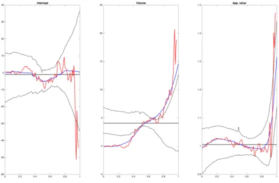
the AQR and ASQR estimators are also smoother than standard quantile regression ones, see for instance Figure 4 in the Application Section.
4
Main results
4.1
Main assumptions and sieve choice
The notations a∨b and a∧b are used instead of max (a, b) and min (a, b). Recall aL bL
means that both aL/bL =O(1) andbL/aL =O(1). The norm k·k is the Euclidean one, i.e.
kek= (e0e)1/2.
4.1.1 General assumptions
Assumption A (i) The auction variables(I`, x`, Vi`, Bi`, i= 1, . . . , I`) are iid across`. The
pdf f(x|I) of the covariates x` given I` = I is continuous and bounded away from 0 over
its bounded support X, with a non empty interior and which does not depend upon I. The actual number of bidders I` belongs to a finite set I of integer numbers larger or equal to 2.
(ii) Given (x`, I`) = (x, I), the Vi`, i = 1, . . . , I` are iid with a conditional quantile
function V (α|x, I), which is continuously differentiable over [0,1]× X with
inf
(α,x,I)∈[0,1]×X ×IV
(1)(α|x, I)>0 and sup (α,x,I)∈[0,1]×X ×I
V(1)(α|x, I)<∞. (iii) (2.3) holds with B(0|x, I) =V (0|x, I) for all (x, I)∈ X × I.
Assumption S For some s ≥ 1 and each I ∈ I, V (α|x, I) is (s+ 1)−times continuously differentiable over [0,1]× X with either: (i) DM = 0 in which case V (α|x, I) = X0γ(α|I)
as in (2.5); (ii) DM >0, in which case V (α|x, I) has DM interactions as in (2.9).
Assumption H The kernel function K(·) with support (−1,1) is symmetric, continuously differentiable over the straight line, and strictly positive over (−1,1). The positive bandwidth h goes to 0 with
lim
L→∞
logL
Lh2(DM+1) = 0.
For the ASQR estimator, P(x) = [P1(x), . . . , PK(x)] 0
where Pk(x) = Phk(x) and K
h−DM. The retained sieve satisfies the high-level Assumption R stated in Appendix A.
Assumption F For all x in X and α in [0,1], the function F[α, x, b0I, b1I;I ∈ I] is twice
differentiable with respect to b0I andb1I, I in I. The partial derivatives of order 1 and 2 are
continuous with respect to α, x, BI and B (1)
I , I in I.
Assumption A recalls the quantile implications of Bayesian Nash equilibrium bidding under symmetric IPV, see Assumption A-(iii). In Assumption A-(i), the existence of a conditional pdf for the covariatex`is only used for the infinite dimensional quantile regression
specification. For a standard quantile regression specification, it is sufficient to assume that the matrix E[I(I` =I)X`X`0] has an inverse for allI ∈ I as recalled in Assumption R-(i) in
Appendix A. Note that, as all along this paper, private values and number of bidders can be dependent. A discussion of such dependence in relation with an entry stage preliminary to the auction can be found in Marmer, Shneyerov and Xu (2013a). For Assumption A-(ii), recall that
V(1)(α|x, I) = 1
f(V (α|x, I)|x, I), (4.3)
wheref(v|x, I) is the conditional private value pdf. Hence Assumption A-(ii) amounts to as-sume thatf(v|x, I) is bounded away from 0 and infinity on its support [V (0|x, I), V (1|x, I)] as assumed for instance in Riley and Samuelson (1981), Maskin and Riley (1984) or GPV.
The condition 0< f(v|x, I)<∞is also used for asymptotic normality of quantile regression estimator, see Koenker (2005). Assumption S combines a standard smoothness assumption with interaction restrictions.
Assumption H restricts the rate at which the bandwidth can go to 0. In the AQR case, it writes limL→∞logL/(Lh2) = 0 which is slightly more restrictive than the condition
limL→∞logL/(Lh) = 0 used in nonparametric estimation. This rate restriction is specific
to the quantile approach used here. The restriction K h−DM and the choice of a sieve satisfying the high-level Assumption R of Appendix A is discussed in the next section.
Assumption F hold for most of the examples of functionals above. A notable excep-tion is the cdf F (v|x, I) in Example 3 when expressed using the rearrangement method of Chernozhukov et al. (2010), which involves an indicator function which is not smooth. How-ever it holds for the smoothed approximation Fη(v|x, I) of the cdf, although Assumption F
implicitly rules out vanishing bandwidth η in Example 3.
4.1.2 Choice of a sieve satisfying Assumption H
The last stage of our procedure is the choice of a suitable sieve in (2.10), when a quantile regression specification cannot be used and more flexibility is needed. While the high level Assumption R of Appendix A mentioned in Assumption H describes some key theoretical properties used in the main results, the focus is set here on suitable sieves. The most important requirement is that the sieve has good approximation properties as detailed in Appendix A. Although not strictly necessary, the sieve functions Pk(·) in the private value
quantile expansion (2.10) should be localized, i.e. the number ofPk0(·) such thatPk(·)Pk0(·)
do not vanish must be bounded. These two requirements are typically satisfied by sieves building on cardinal spline basis or wavelets as detailed now.
Consider first the spline example of sieves. Assume that X = [0,1]D for the sake of brevity. Form ≥s+ 2, set (t)m+−1 =tm−1 ift >0 and (t)m−1
+ = 0 otherwise. The considered
(Schumaker (2007), p.135) q(t) = m X i=0 (−1)i mi(t−i)m+−1 m!
which has m−2 continuous derivatives over the straight line and which support is [0, m]. The baseline B−spline functionq(·) generates the rescaled functions pκh(·) =pκ(·)
pκ(t) = 1 √ hq t−(κ−m)h h , κ= 1, . . . , κ
where κ = κh = O(1/h) is the largest integer number such that (κ−m)h ≤ 1 ≤ κh.
Theorem 6.20 in Schumaker (2007) implies that each function v(·) with s+ 1 continuous derivatives can be approximated uniformly over [0,1] with a linear combination of thepκ(·)’s
up to an error o h−(s+1). The pκ(·)’s are also localized with
R1
0 p 2
κ(t)dt =O(1) uniformly
inκ and h. Similarly, additive quantile functions as in (2.8) can be approximated using the sieve
{pκ(x1), . . . , pκ(xD), κ= 1, . . . κ}.
A suitable sieve for additive interactive quantile function of order DM as in (2.9) is
(DM Y δ=1 pκδ(xjδ), all (κδ, jδ) with 1 ≤κ1, . . . , κDM ≤κ, 1≤j1 <· · ·< jδ ≤D ) . (4.4) The set (4.4) can be written as a collection {Pk(x), k= 1, . . . , K} with K = O h−DM
localized functions satisfying RX P2
k(x)dx=O(1) uniformly ink and h.
Similar localized sieve can be obtained using wavelets on the interval [0,1], see H¨ardle, Kerkyacharian, Picard and Tsybakov (1998), Chen (2007) and the references therein, in particular Daubechies (1992). Let ϕ(·) and ψ(·) the father and mother wavelets of order
the collection of functions DM Y δ=1 1 2−H0/2ϕ xjδ −2 −H0κ δ 2H0 and DM Y δ=1 1 2−H/2ψ xjδ −2 −Hκ δ 2H , H0 ≤H ≤H1
where H0 and H1 are two diverging integer numbers with 2−H h, κδ and jδ as in (4.4).
4.2
Private value quantile estimation results
The next sections give our theoretical results for integrated mean squared error and asymp-totic distribution of the augmented estimator Vb(·|x, I). Theorem A.1 in Appendix A also gives uniform consistency rates of similar interest.
4.2.1 Integrated mean squared error
Recall P (x`) = [1, x0`] 0
is of the constant dimension K =D+ 1 in the AQR case. Let s1 be
the 1×(s+ 2) selection vector (0,1,0, . . . ,0), which is such that s1⊗IdKβb(α|I) = βb1(α|I) is the estimator of sieve coefficient derivative β(1)(α). Let Π1(α) be the second column of
the inverse ofR π(t)π(t)0K(t)dt, i.e., Π1(α) = Z π(t)π(t)0K(t)dt −1 s10
and consider the variance terms
v2(α) = Π1(α)0 Z Z π(t1)π(t2) 0 min (t1, t2)K(t1)K(t2)dt1dt2Π1(α), Σ (α|I) = α 2v2(α) (I−1)2E −1 P (x`)P(x`) 0 I(I` =I) B(1)(α|x `, I`) ×E P (x`)P (x`) 0 I(I` =I) E−1 P (x`)P(x`) 0 I(I` =I) B(1)(α|x `, I`) , ΣIL= Z X Z 1 0 P(x)0Σ (α|I)P (x)dαdx.
That v2(α), and then ΣIL, is strictly positive follows from the proof of Theorem 2 below,
see in particular Lemma B.5 in Appendix B. The bias of the estimator will depend upon
Bias(α|I) = α I−1s1 Z π(t)π(t)0K(t)dt −1Z ts+2π(t) (s+ 2)!K(t)dt ×E−1 P (x`)P (x`) 0 I(I` =I) B(1)(α|x `, I`) E I(I` =I)P (x`)αB(s+2)(α|x`, I`) B(1)(α|x `, I`) , Bias2IL= Z X Z 1 0 P (x)0Bias(α|I)2 dαdx.
Theorem 2 Suppose that the private value conditional quantile function V (·|·) is a quantile regression (2.5), for which DM = 0, or a sieve quantile regression (2.10) with DM
inter-actions. Then under Assumptions A, H, S with s ≥ DM/2, there exists an approximation
b v(α|x, I) of Vb(α|x, I) such that E Z X Z 1 0 (bv(α|x, I)−V (α|x, I))2dαdx =h2(s+1)Bias2IL+ ΣIL LIhDM+1 +o h2(s+1)+ 1 LhDM+1
where Bias2IL =O(1), ΣIL=O(1) and
Z X Z 1 0 b V (α|x, I)−vb(α|x, I) 2 dαdx=oP 1 LhDM+1 . (4.5) The quantile estimator Vb(α|x, I) is nonlinear and defined in an implicit way, so that attempting a direct computation of its IMSE is difficult. Its approximationbv(α|x, I) follows from a Bahadur linearization argument, see Theorem D.1 and (E.1) in Appendices D and E. The rate in equation (4.5) is negligible with respect to the IMSE of bv(α|x, I), showing that it is fair to replace Vb(α|x, I) by bv(α|x, I) to picture the IMSE of Vb(α|x, I).
Note that Theorem 2 holds over the full quantile level range [0,1]. The bias variance decomposition of the IMSE is driven by the estimation of αB(1)(α|x, I) in V (α|x, I) =
B(α|x, I) +αB(1)(α|x, I)/(I−1), a function which is (s+ 1)th continuously differentiable
bias component due to the estimation of B(α|x, I) is of the negligible orderhs+2 except per-haps over a small vicinity of 0 where it iso(hs+1). The asymptotic variance Σ
IL/ LIhDM+1
order is similar to the asymptotic variance obtained for kernel estimation of a conditional pdf withDM covariates. Indeed, the bid quantile derivative is homogeneous to a conditional
pdf since
B(1)(α|x, I) = 1
g[B(α|x, I)|x, I],
where g(·|·) is the bid conditional pdf. The bid quantile function is homogeneous to a cdf and converges with a faster rate. Note that the asymptotic variance term ΣIL/ LIhDM+1
depends upon the number of interactions DM and not the dimension of the covariate D.
Hence Theorem 2 illustrates the dimension reduction features of the procedure. In particular, the variance term is of order 1/(Lh) in the AQR case independently of the dimension of the covariate D, which therefore can be large.
Maximizing the leading term of the IMSE yields the optimal bandwidth
h∗ = (DM+ 1) ΣIL 2 (s+ 1)Bias2IL 1 LI 2s+D1 M+3 . (4.6)
As in kernel estimation, a pilot bandwidth can be computed using a simple private value quantile regression model to proxy ΣIL and Bias2IL in a parametric way. The corresponding
IMSE rate is
L
s+1 2s+DM+3
which decreases with the number of interactions DM, but does not depend upon the
dimen-sionDof the covariate. In the AQR case with DM = 0, the IMSE rateL
s+1
2s+3 is, as expected,
the optimal rate for estimating the marginal pdf of a real random variable. For s= 1, it is equal to L2/5 independently of the dimension D of the covariate, which is close of L1/2.
Two assumptions limit the use of the optimal bandwidth (4.6). First, Theorem 2 assumes
s≥DM/2 but this condition is only binding for a number of interactions DM larger than 3
since s ≥1 under Assumption S. Belloni et al. (2017) have a similar restriction for a sieve quantile estimator. In a context where the covariateDreplacesDM but plays a similar role,
Aryal et al. (2016) however use a condition s+ 1 > D to study a GMM version of GPV based on a local polynomial estimation of the private value.
4.2.2 Central limit theorem
This section states a Central Limit Theorem for Vb(α|x, I), Theorem 3, which illustrates the good pointwise properties of Vb(α|x, I) near or at the upper boundaryα = 1. Lets1 be the selection vector defined earlier and
Π1h(α) = Z 1−hα −α h π(t)π(t)0K(t)dt !−1 s10, v2h(α) = Π1h(α)0 Z 1−hα −α h Z 1−hα −α h π(t1)π(t2) 0 min (t1, t2)K(t1)K(t2)dt1dt2Π1h(α), Σh(α|I) = α2v2 h(α) (I−1)2E −1 P (x`)P(x`) 0 I(I`=I) B(1)(α|x `, I`) ×E P (x`)P(x`) 0 I(I` =I) E−1 P (x`)P (x`) 0 I(I` =I) B(1)(α|x `, I`) , (4.7) Biash(α|I) = α I−1s1 Z 1−hα −α h π(t)π(t)0K(t)dt !−1 Z 1−hα −α h ts+2π(t) (s+ 2)!K(t)dt ×E−1 P (x`)P (x`) 0 I(I` =I) B(1)(α|x `, I`) E I(I` =I)P (x`)αB(s+2)(α|x`, I) B(1)(α|x `, I) . (4.8)
Theorem 3 Suppose that the private value conditional quantile function V (·|·) is a quantile regression (2.5) or a sieve quantile regression (2.10) with DM interactions. Then under
Assumptions A, H, S with s≥DM/2 and
log2L
it holds for α in (0,1] and all x in X that LIh P(x)0Σh(α|I)P (x) 1/2 b V (α|x, I)−V (α|x, I)−hs+1P(x)0Biash(α|I) +o hs+1
converges in distribution to a standard normal. Moreover P (x)0Σh(α|I)P(x) αh−DM
and max(α,x)∈[0,1]×X P(x) 0 Biash(α|I) =O(1).
Theorem 3 shows that the asymptotic variance of Vb(α|x, I) is of order α/ LhDM+1
for
α >0. For α = 0, Vb(α|x, I) =Bb(α|x, I) has an asymptotic variance of order 1/ LhDM+1
and a corresponding CLT using this standardization also holds. For other quantile levels the private value conditional quantile estimator depends upon Bb(1)(α|x, I) so that the asymp-totic variance of Vb(α|x, I) has the larger order 1/ LhDM+1
which also holds in Theorem 2. The expression of the asymptotic variance of Vb(α|x, I) is quite typical of quantile regression estimators, up to the factor v2h(α) which is due to Bb(1)(α|x, I).
It follows from Theorem 3 that the private value conditional quantile estimator is con-sistent for all quantile levels, including α = 1. The potential boundary effects only appear through the bias and variance factors Biash(α|I) and Σh(α|I). Since the support of the
kernel is [−1,1], it holds that
Biash(α|I) = Bias(α|I) and Σh(α|I) = Σ (α|I) for all α in [h,1−h]
whereBias(α|I) and Σ (α|I) are defined before Theorem 2, allowing in principle to implement simple pilot bandwidth for quantile level inside [0,1]. Whenα lies in (0, h] or [1−h,1], the bias and variance factors depend upon h. It is commonly believed that the variance factor is inflated near the boundaries but there is no clear result for the bias factor, see Fan and Gijbels (1996) and the references therein.
4.3
Functional estimation
The plug in estimators of θ(x) and θ in (2.13) are b θ(x) = Z 1 0 Fhα, x,Bb(α|x, I),Bb(1)(α|x, I) ;I ∈ I i dα, θb= Z X b θ(x)dx,
with AQR or ASQR Bb(α|x, I) and Bb(1)(α|x, I). Alternatively, θ can be estimated using PL
`=1θb(x`)/L. Let us now introduce the asymptotic variances ofθb(x) and bθ. The variances depend upon the matrices
P(I) =E[I(I` =I)P (x`)P (x`)], P0(α|I) =E I(I` =I)P(x`)P (x`) B(1)(α|x `, I`) ,
and of the functions, recalling b0I and b1I stand for B(α|x, I) and B(1)(α|x, I) respectively,
ϕ0I(α, x) = ∂F α, x, B(α|x, I), B(1)(α|x, I) ;I ∈ I ∂b0I , ϕ1I(α, x) = ∂F α, x, B(α|x, I), B(1)(α|x, I) ;I ∈ I ∂b1I .
LetA be a random variable with the uniform distribution over [0,1] and define
σL2(x|I) = ITr Var Z A 0 ϕ0I(α|x)− ∂ϕ1I(α|x) ∂α P0(α|I) −1 dα P(I)1/2hDM/2P (x) , σL2(I) = ITr Var Z A 0 Z X ϕ0I(α|x)− ∂ϕ1I(α|x) ∂α P0(α|I) −1 P1/2(I)P (x)dx dα , σL2(x) = X I∈I σ2L(x|I), σL2 =X I∈I σL2(I).
The proof of Theorem 4 in Appendix E shows that the asymptotic variances of bθ(x) and θb are σ2 L(x)/ LhDM and σ2 L/Lrespectively provided ϕ0I(α|x)6= ∂ϕ1I(α|x) ∂α (4.9)
for some α, x and I of [0,1]× X × I. Indeed, if ϕ0I(α|x) = ∂ϕ1I(α |x)
∂α for all α and I,
σ2
L(x|I) = 0 and, if this also holds for all x, σL2 = 0, in which case bθ(x) and θbcan converge to θ(x) and θ with “superefficient” rates, faster than LhDM1/2 and L1/2 respectively. In the case of density based functionals, Laurent (1997) similarly obtained asymptotic variance that can vanish. Why it is possible is better understood in our quantile context, through an example of functionals for which (4.9) does not hold.8 Consider, for some I
0 of I, F1 α, x, B(α|x, I), B(1)(α|x, I) ;I ∈ I = 2B(α|x, I)B(1)(α|x, I0) which gives (ϕ0I0(α|x), ϕ1I0(α|x)) = 2 B (1)(α|x, I 0), B(α|x, I) . Henceϕ0I(α|x) = ∂ϕ1I(α|x) ∂α
for all (α, x, I), so that (4.9) does not hold and σ2
L(x) =σL2 = 0. Why θb(x) and θbcan con-verge with superefficient rates for these functionals is in fact not surprising observing that they estimate
θ1(x) =B2(1|x, I0)−B2(0|x, I0), θ1 =
Z
X
θ1(x)dx,
respectively. Hence, for these examples, the parameters of interest only depend upon extreme quantiles, in which case superefficient estimation is possible, see e.g. Hirano and Porter (2003) and the references therein. A role of the new Condition (4.9) is to exclude such functionals. The next Theorem establishes the asymptotic normality of bθ(x) and θb.
Theorem 4 Suppose Assumptions A, F, H, S and R hold withs ≥DM/2. Thenσ2L(x)and
σ2
L are bounded away from 0 and infinity if (4.9) holds for some (α, I) in [0,1]× I and for
some (α, x, I) in [0,1]× X × I respectively. Moreover
i. If logL Lh2DM+2+(DM∨1) =o(1), √ LhDM b θ(x)−θ(x)−biasL,θ(x) /σL(x)converges in
dis-tribution to a standard normal, where biasL,θ(x) is a o(hs) bias term.
ii. If logL
Lh2DM+1+(DM∨1) =o(1),
√
Lθb−θ−biasL,θ
/σLconverges in distribution to a
stan-dard normal, where biasL,θ is a o(hs) bias term.
8A more systematic study is out of the scope of the present paper, as is the issue of semiparametric
The bias term order is given by the estimation ofB(1)(α|x, I). WhenF(·) depends upon
αB(1)(α|x, I) as in all the Examples, the exact order of the bias term ishs+1 with
biasL,θ(x) =hs+1(1 +o(1)) X i∈I Z 1 0 Gb1I α, x, B(α|x, I), αB(1)(α|x, I) ;I ∈ I ×P (x)0Biash(α|x, I)dα and biasL,θ = R
XbiasL,θ(x)dx where Biash(α|x, I) is as in (4.8) and Gb1I(·) is the partial
derivative of F(·) with respect to αB(1)(α|x, I). θb(x) or θbare therefore asymptotically unbiased if hs+1√LhDM = o(1) or hs+1√L = o(1) respectively. The items Bias
h(α|x, I)
in the integral expression of biasL,θ(x) can be replaced with their limits Bias(α|x, I) defined
before Theorem 2. Theorem 4 applies to our functional Examples as follows.
Example 1 (cont’d). Letθb=θbn/θbd be the CRRA risk aversion plug in estimator derived from (2.15). Under the bandwidth condition of Theorem 4-(ii),θbn=θn+biasL,θn+OP L−1/2
and θbd=θd+biasL,θd +OP L−1/2
. A standard linearization argument then gives that the asymptotic distribution of √ L b θ−θdbiasL,θn −θnbiasL,θn θ2 d is the one of θd √ Lθbn−θn −θn √ Lθbd−θd θ2 d
which is normal, applying Theorem 4-(ii) with
F α, x, B(α|x, I), B(1)(α|x, I) ;I ∈ I = B(α|x, I1)−B(α|x, I0) θd αB(1)(α|x, I 0) I0−1 −αB (1)(α|x, I 1) I1 −1 − θn θ2 d αB(1)(α|x, I 0) I0−1 − αB (1)(α|x, I 1) I1−1 2 .
The functions ϕ0I(α|x)−∂ϕ1I(α |x)
∂α appearing in the asymptotic variances are, for I =I1,
ϕ0I1(α|x)− ∂ϕ1I1(α|x) ∂α = 1 θd αB(1)(α|x, I0) I0−1 − αB (1)(α|x, I 1) I1−1 − B(α|x, I1)−B(α|x, I0)−α B (1)(α|x, I 0)−B(1)(α|x, I1) θd(I1−1) + 2θn θ2 d(I1−1) αB(1)(α|x, I0) I0−1 − αB (1)(α|x, I 1) I1−1 + 2θnα θ2 d(I1−1) B(1)(α|x, I0) +αB(2)(α|x, I0) I0−1 − B (1)(α|x, I 1) +αB(2)(α|x, I1) I1 −1
where αB(2)(α|x, I) is well defined over [0,1] by (2.3). The case I = I
0 is similar. Using
these expressions to estimate the asymptotic variance CRRA risk-aversion θbis difficult due to the second derivative B(2)(α|x, I), which is difficult to estimate. Although not formally
studied here, using a bootstrap procedure may be more appropriate.
Example 2 (cont’d). Theorem 4-(i) together with Theorem 3 are useful to study the plug in estimatorERd(αR|x, I) derived from (2.17). Theorem 4-(i) gives that the estimator of the integral component θ(x;αR) satisfies θb(x;αR) = θ(x;αR) + O(hs+1) + OP
1/√LhDM,
while Theorem 3 ensures that Vb(α|x, I) = V (α|x, I) +O(hs+1) +OP
1/√LhDM+1. As
the O(hs+1) items correspond to bias terms and theOP(·) ones are given by the estimation stochastic component, bothθb(x;αR) and Vb(αR|x, I) contribute to the bias ofERd(αR|x, I).
The asymptotic distribution of the bias centered √LhDM+1
d
ER(αR|x, I)−ER(αR|x, I)
is the one of IαIR−1(1−αR)
√
LhDM+1
b
V (αR|x, I)−V (αR|x, I)
, which follows from The-orem 3. The uniform consistency TheThe-orem A.1 in Appendix A can be used to study the estimated screening level αbR(x, I) and reserve priceVb(αbR(x, I)|x, I) obtained by
maximiz-ing ERd(αR|x, I).
Example 3 (cont’d). Theorem 4-(i) is also useful to study the private value cdf. and pdf, estimator from Example 3, with a fixed bandwidth η. The proof carries over if η goes to 0
with h =o(η) and the order of the variance given by Theorem 4-(i) is correct if η is of the order of η. For the cdf estimator Fbη(v|x, I) =
R1 0 Iη h v−Vb(α|x, I) i dα, ϕ0I(α|x) = − 1 ηk v−V (α|x, I) η , ϕ1I(α|x) = α (I−1)ηk v−V (α|x, I) η , ∂ϕ1I(α|x) ∂α = 1 (I−1)ηk v−V (α|x, I) η − α (I−1)η2k (1) v−V (α|x, I) η V(1)(α|x, I).
When ηgoes to 0, the dominant part of the variance is, for inner v, integrating by parts and setting Vx,I =V (A|x, I)
I LhDM Tr Var Z A 0 ∂ϕ1I(α|x) ∂α P0(α|I) −1 dα P(I)1/2hDM/2P(x) = (1 +o(1))I LhDM Tr ( Var " ϕ1I(A|x) ∂P0(A|I) −1 ∂α P(I) 1/2 hDM/2P (x) #) = (1 +o(1))I (I−1)2LhDM ×Tr Var F (Vx,I|x, I) f(Vx,I|x, I) kv−Vx,I η η ∂P0(F (Vx,I|x, I)|I) −1 ∂α P(I) 1/2 hDM/2P(x) = (1 +o(1))I R k2(t)dt (I−1)2LηhDM F(v|x, I) f(v|x, I) 2 ×Tr ( ∂P0(F (v|x, I)|I) −1 ∂α P(I) 1/2 hDMP (x)P (x)0P(I)1/2 ∂P0(F (v|x, I)|I) −1 ∂α ) .
Hence the order of the variance of Fbη(v|x, I) is 1/ LηhDM
. Its bias as an estimator of
F (v|x, I) has two components: the first is biasL,Fη(v|x,I) due to the bias of Vb(α|x, I) and is
of order O(hs+1), while the second is F
η(v|x, I)−F (v|x, I) = O(ηs+1) is k(·) is a kernel
of order s. It follows that the optimal bandwidths h and η must have the same order
L−1/(2s+DM+3) which gives the consistency rate L−(s+1)/(2s+DM+3). Repeating these steps for
the pdf estimator fbη(v|x, I) gives the same optimal consistency rate L−s/(2s+DM+3) which,
up to a logarithmic term, corresponds to the GPV optimal minimax rate in presence of DM
5
Simulation experiments
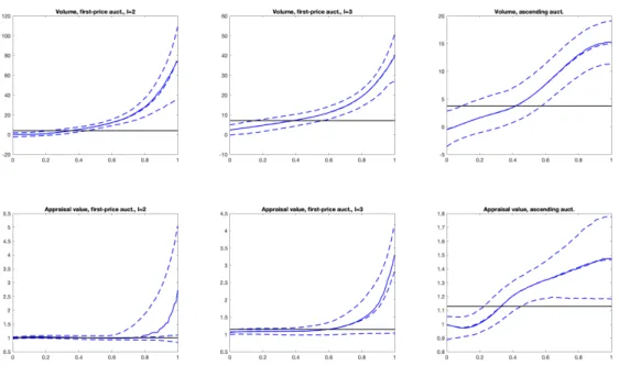
This section reports the results of a simulation experiment for the AQR estimation of the private value quantile function, the expected revenue and optimal reserve price under risk neutrality from first-price auction with I = 2. A second simulation experiment considers estimation of risk aversion based on comparison of first-price auctions withI = 2 andI = 3 as in (2.15) and on comparison with first-price and ascending auctions with I = 2. In each case, the considered number of auctions is L= 100 and the number of replications is 1,000. As the most difficult component to estimate in the private value quantile function is
αB(1)(α|x, I)/(I−1), choosing I = 2 corresponds to a worst case scenario. By contrast,
the simulation experiment in GPV considersI = 5 whileI = 3 or 5 in Marmer and Shneyerov (2012) and Ma, Marmer and Shneyerov (2018). The number of bids in these references range from 1,000 for GPV to 4,200 for Marmer and Shneyerov (2012). In a simulation experi-ment focused on the nonparametric estimation of the utility function of risk averse bidders, Zincenko (2018) considers I = 2 with L = 300 and I = 4 with L = 150. Our simulation experiment is therefore more focused on small samples. We also use three covariate while the aforementioned simulation experiments do not consider covariate, with the exception of Zincenko (2018) who increases the number of auctions to L= 900 for one or two covariates to cope with the curse of dimensionality.
5.1
Model and estimation method
The private value quantile function is given by a quantile regression model with an intercept and three independent covariates with the uniform distribution over [0,1],
with
γ0(α) = 1 + 0.5 exp(5(α−1)), γ1(α) = 1,
γ2(α) = 0.5(1−exp(−5α)), γ3(α) = 0.8 + 0.15((2π+ 1)α+ cos(2πα)).
The coefficientγ0(·) is flat near 0 and fastly increases near 1, as observed in the application
displayed in the next section, while γ2(·) fastly increases near 0 and is flat after. The
derivative ofγ3(·) has some oscillating patterns.
The expected revenue ER(α) is computed from (2.17) setting the intercept, x1 and x3
to 0 and taking x2 = 0.8. This choice gives a unique optimal reserve price achieved for
α =.3, which is not too close to the boundaries so that the expected revenue function has a substantial concave shape which is suppose to make estimation more difficult.
5.2
Private value and expected revenue
The private value quantile regression is estimated from a sample of 100 first-price auctions with two bids over the estimation grid α = 0,0.01, . . . ,0.99,1 with an augmented quan-tile regression estimator Vb(α|x) of order 2 and kernel K(t) = 6t(1−t)I(t ∈[0,1]). The expected revenue estimator dER(α) plugs 0.8bγ2(α) into (2.17) using Riemann sums to
com-pute integrals. The optimal screening level αb∗ maximizes ERd(α) over the grid and is used to compute the estimated optimal reserve price Rb∗ = .8bγ2(αb∗) and the estimated optimal revenue ERd∗ =ERd(
b
α∗).
Table 1 summarizes the simulation results for the estimation of the private value quantile function, the expected revenue and the optimal reserve price. The Bias and Square Root Integrated Mean Squared Error (RIMSE) lines for Vb(·|·) gives the simulation counterparts of, respectively 1 4 3 X j=0 Z 1 0 (E[bγj(α)]−γj(α)) 2 dα !1/2 and 1 4 3 X j=0 Z 1 0 E(bγj(α)−γj(α)) 2 dα !1/2 .
The Bias and RIMSE for the expected revenue are computed similarly. Table 1 also gives the Bias and Mean Squared Error (MSE) of the optimal reserve price estimator. All these quantities are computed for bandwidths .2, .3, . . . , .9.
h .2 .3 .4 .5 .6 .7 .8 .9 b V (·|·) Bias .131 .141 .143 .145 .150 .159 .166 .176 RIMSE .433 .386 .355 .332 .322 .309 .303 .305 d ER(·) Bias .036 .044 .049 .050 .051 .049 .047 .045 RIMSE .109 .104 .102 .100 .099 .098 .097 .096 b R∗ Bias -.036 -.031 -.014 -.002 .009 .022 .037 .043 RMSE .129 .099 .075 .067 .062 .064 .066 .066
Table 1: Private value quantile function, expected revenue, and optimal reserve price
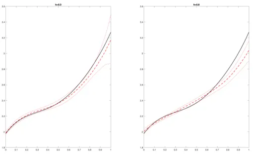
Figure 2: Private value quantile estimation forh= 0.3 (left) andh= 0.8 (right) for average covariate. True V(α|x) = γ0(α) + (γ1(α) +γ2(α) +γ3(α))/2 in black. Dashed red line:
average estimation. Dotted red line: pointwise 2.5% −97.5% quantiles of Vb(α|x) across 1,000 simulations.
Estimation of the private value slope coefficients seems much more sensitive to the band-width parameter than the expected revenue or optimal reserve price. It has also a much higher RIMSE. The bandwidth behavior of Vb(α|x) is illustrated in Figure 2, which
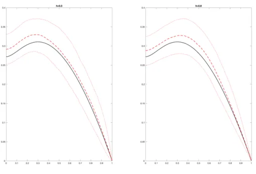
consid-Figure 3: Expected revenue estimation for h= 0.3 (left) andh = 0.8 (right). True ER(α|x) in black. Dashed red line: average estimation. Dotted red line: pointwise 2.5%−97.5% quantiles of ERd(α|x) across 1,000 simulations.
ers the small bandwidth h= 0.3 and the larger h = 0.8. As expected from Theorem 3, the variance ofVb(α|x) increases withαand decreases withh, while the bias increases withαbut decreases with h. Figure 2 also suggests that choosing a large bandwidth as recommended by Table 1 may lead to important bias issues, including underestimating the private value quantile function for high α.
This contrasts with estimation of the expected revenue and optimal reserve price, which seems mostly unaffected by the bandwidth. This is because the expected revenue depends upon (1−α)V (α|x): multiplying the private value quantile function by (1−α) mitigates larger bias and variance near the boundary α = 1, see also Figure 3. For the considered experiment, the true expected revenue is always in the 95% band of Figure 3 while the true private quantile function is out for large α when h= 0.8.
5.3
CRRA risk aversion
Two risk aversion estimators are considered. The first estimatorθbf p is based upon (2.15) and
uses two independent samples of size L = 100 with 2 and 3 bidders from the model above, which corresponds to a CRRA utility functionxθ withθ = 1.9 Integrals with respect toαare computed using Riemann sums whereas integrals with respect toxare replaced with sample means over the two auction samples. The second estimator θbasc is based upon (2.16) and
uses an additional sample of size L = 100 of ascending auctions with two bidders. In this case, it is possible to consider various values ofθ and the simulation experiment considers the values 0.2, 0.6 and 1. Indeed, if B(α|x) is the first-price auction quantile bid function with
I = 2, the observed bids drawn fromB(α|x) are rationalized by a CRRA utility functionxθ
if the private value quantile function is set to
Vθ(α|x) = B(α|x,2) +θαB(1)(α|x,2)
provided Vθ(1)(·|x) > 0 for all x as seen from Campo et al. (2011) and (2.14) here. As
Vθ(1)(·|·) > 0 holds in our case, we use Vθ(α|x) to generate two ascending bids for each
auction. Following Gimenes (2017), Vθ(α|x) can be estimated from winning bids in these
ascending auction using AQR for quantile level 2α−α2 instead ofα.
The performance of the two estimators are summarized in the next Table. Table 2 shows
θ h .2 .3 .4 .5 .6 .7 .8 .9 b θf p 1 Bias -.795 -.564 -.412 -.288 -.178 .-.080 .003 .053 RMSE .891 .681 .545 .471 .404 .380 .393 .436 b θasc 1 Bias -.016 -.019 -.037 -.061 -.085 -.100 -.109 -.111 RMSE .240 .247 .248 .254 .260 .267 .276 .282 .6 Bias .028 .023 .009 -.008 -.025 -.035 -.040 -.042 RMSE .172 .176 .174 .175 .175 .179 .184 .188 .2 Bias .088 .083 .075 .066 .058 .053 .052 .053 RMSE .135 .133 .126 .122 .117 .116 .116 .118 Table 2: Risk aversion estimation
9The optimal bid functions can be computed explicitly under the risk neutrality caseθ= 1. Considering