Parameter Estimation In Weighted Rayleigh Distribution

Volume 16 | Issue 2 Article 14

December 2017

Parameter Estimation In Weighted Rayleigh

Distribution

M. Ajami

Vali-e-Asr University of Rafsanjan, Rafsanjan, Iran, [email protected]

S. M. A. Jahanshahi

University of Sistan and Baluchestan, Zahedan, Iran, [email protected]

Follow this and additional works at:http://digitalcommons.wayne.edu/jmasm

Part of theApplied Statistics Commons,Social and Behavioral Sciences Commons, and the

Statistical Theory Commons

This Regular Article is brought to you for free and open access by the Open Access Journals at DigitalCommons@WayneState. It has been accepted for Recommended Citation

Ajami, M., & Jahanshahi, S. M. A. (2017). Parameter Estimation In Weighted Rayleigh Distribution. Journal of Modern Applied Statistical Methods, 16(2), 256-276. doi: 10.22237/jmasm/1509495240

M. Ajami is an Assistant Professor in the Department of Statistics. Email him at

[email protected]. S. M. A. Jahanshahi is a Professor in the Department of Statistics. Email him at [email protected].

Parameter Estimation In Weighted

Rayleigh Distribution

M. Ajami

Vali-e-Asr University of Rafsanjan Rafsanjan, Iran

S. M. A. Jahanshahi

University of Sistan and Baluchestan Zahedan, Iran

A weighted model based on the Rayleigh distribution is proposed and the statistical and reliability properties of this model are presented. Some non-Bayesian and Bayesian methods are used to estimate the β parameter of proposed model. The Bayes estimators are obtained under the symmetric (squared error) and the asymmetric (linear exponential) loss functions using non-informative and reciprocal gamma priors. The performance of the estimators is assessed on the basis of their biases and relative risks under the two above-mentioned loss functions. A simulation study is constructed to evaluate the ability of considered estimation methods. The suitability of the proposed model for a real data is shown by using the Kolmogorov-Smirnov goodness-of-fit test.

Keywords: Bayesian estimators, estimation methods, goodness-of-fit, loss function, reliability, weighted model

Introduction

The Rayleigh distribution has been used in many areas of research, such as reliability, life-testing and survival analysis. Modeling the lifetime of random phenomena has been another area of study for which the Rayleigh distribution has

been significantly used. Being first introduced by Rayleigh (1880), this statistical

model was originally derived in connection with a problem in acoustics. More details on the Rayleigh distribution can be found in Johnson et al. (1994) and references therein.

The Rayleigh distribution has the following probability density function (pdf) and the cumulative distribution function (cdf), respectively,

 

 

2 2 exp , 0, 0, 2 1 exp , 0, 0. 2 x x f x x x F x x         _ _         _ _    

Weighted distributions are employed mainly in research associated with reliability, bio-medicine, meta-analysis, econometrics, survival analysis, renewal processes, physics, ecology and branching processes which are found in Patil and Rao (1978), Gupta and Kirmani (1990), Gupta and Keating (1985), Oluyede

(1999), Patil and Ord (1976) and Zelen and Feinleib (1969). A weighted form of

Rayleigh distribution has been published by Reshi et al. (2014). They introduced a

new class of Size-biased Generalized Rayleigh distribution and also investigated the various structural and characterizing properties of that model. In addition, they studied the Bayes estimator of the parameter of the Rayleigh distribution under the Jeffrey’s and the extended Jeffrey’s priors assuming two different loss functions. They compared four estimation methods by using mean square error through simulation study with varying sample sizes. In fact, weighted distributions arise in practice when observations from a sample are recorded with unequal probabilities

Suppose X is a non-negative random variable with its unbiased pdf f(x,β), β is a parameter, then g distribution is weighted version of f and is defined as







_

,

_

 

,

_

_



, , , , w x f x g x E w X





 





where the weight function w(x,α) is a non-negative function and 0 < E(w(X,α)) is a normalizing constant which is E(w(X,α)) = ∫w(x,α)f(x,β)dx. Furthermore, α is a parameter which may or may not depend on β and E(w(X,α)) = 1/Eg(1/w(X,α)) is

the harmonic mean of w(x,α) with the pdf g(.).

When w(x,α) = xα, α = 0, the distribution is referred to as weighted distributions of order α.



, ,



x f x

_{ }



,



. g x E X  



 

 (1)

For α = 1 or 2, the pdf (1) are referred to as length-biased (size-biased) and area-biased distributions, respectively.

A weighted Rayleigh (WR) distribution is proposed based on (1) and all calculations are done based upon this model, but in the sections of numerical simulations and application to real data a length-biased Rayleigh (LBR)

distribution is used without loss of generality. Because determinig the value of α

depends on the sampling method so it is not necessary to estimate α in practice,

therefore the focus on estimating the β parameter.

Weighted Rayleigh distribution

In the following, the WR(α,β) distribution is introduced and then, some properties including the rth _{moment, the corresponding CDF and hazard rate function are}

calculated.

Definition 1. A nonnegative random variable X is said to have the WR(α,β) distribution provided that the variable’s density function is given by





_

_

₁ 2_/2 /2 /2 1 1 , , , 0, , 0. 2 / 2 1 x g x  _{ } x e  x             (2)

Remark 1. Suppose that X follows WR(α,β) and let U = X2_/2β,

then U follows Γ(α/2+1,1) distribution.

Remark 2. The WR(α,β) distribution belongs to the exponential family. Therefore, T = Σni=1X2i is a sufficient complete statistic.

The rth _{moments are useful for inference and model fitting. A result that}

allows us to compute the moments of the WR(α,β) distribution is given in the following lemma.

Lemma 1. If X be a random variable with density function (2), then the rth _{moment is given by}

 

/ 2 / 2 1 2 2 , 1 2 r r r r E X       _  _      _  _  

where r is a positive integer.

Proof. According to (2)

 

_

1

_

2_{/ 2} /2 /2 1 0 _{2 / 2 1} , r r x x E X e dx   

_



_

   _    



let x2_{/2β = u}2_{, then we have}

 

 

_

_

₁ 2 _{/ 2 / 2} / 2 / 2 1 ₀ 1 2 2 ₂ 2 . 2 / 2 1 1 2 r r r u r r r E X u e du              _{  }     _  _       _ _     



∎ Lemma 1 concludes

 

1/ 2 1/ 2 1 1 2 2 , 1 2 E X       _  _      _  _  

 

2 2 1 1 1 2 2 2 , 1 1 2 2 V X











 _{      }       _{    }       _{ }   _  _                    _{     }   

 

2 2 1 1 1 1 2 2 2 . 1 1 2 CV X             _  _{ }   _{ }  _           _  _  

The corresponding CDF of the WR(α,β) distribution is as follows:

 

_

_

2_{/ 2}

_

_





/2 1 2 0 1 1 / 2 1, / 2 , / 2 1 / 2 1 x G x  t e dt

 

x









    



  where

 

1 1 0 , z a a z t e dt  _



 

denotes the lower incomplete gamma function.

In addition, the survival and the hazard rate functions of the WR(α,β) distribution are

 

_

_

2

_

_





/2 2 1 / 2 1 1 / 2 1, / 2 , / 2 1 / 2 1 t x G x t e dt x        _     



  and

 

/ 2 / 2 1

_

1 2/ 2 2

_

1 , 2 / 2 1, / 2 x x e h x x   

_



_{ }

_

     respectively, where 1

 

, 1 1 a z a z t e dt  _   



denotes upper incomplete gamma

function.

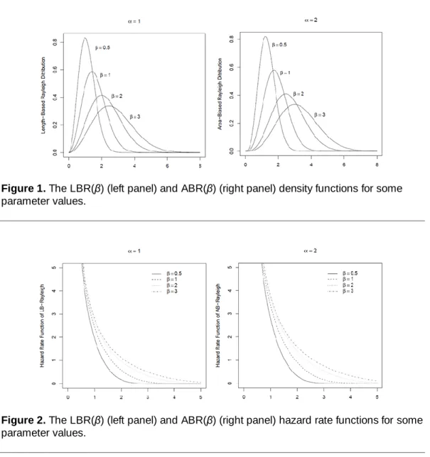
In special cases, if α = 1, corresponding length-biased distribution is

 

2 2_/2 3/2 2 , 0, 0, x x g x e  x



 

   

and if α = 2 corresponding area-biased distribution is

 

3 2_{/ 2} 2 , 0, 0. 2 x x g x e  x





   

Plots of length-biased and area-biased (ABR) distributions for some

parameter values are displayed in Figure 1. Some possible shapes of the LBR and

Figure 1. The LBR(β) (left panel) and ABR(β) (right panel) density functions for some parameter values.

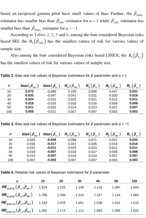
Figure 2. The LBR(β) (left panel) and ABR(β) (right panel) hazard rate functions for some parameter values.

Parameter estimation

In this section, the method of moments, the maximum likelihood method, uniformly minimum variance unbiased method, maximum goodness-of-fit method

Method of moments estimator

Hereafter, let X1, …, Xn be a random sample from the WR(α,β) distribution. The

method of moments estimator (MME) is

2 2 1 2 ˆ _. 1 2 1 2 MME X     _ _      _{ }        _{ }     _{ }  

Maximum likelihood estimator The likelihood function can be written as





_

_

2 1 1 2 1 / 2 / 2 1 1 1 ; , , , 0, , 0. 2 / 2 1 n i i X n n n i i L



x x _{ } X e  x

 





         _ _      



One can easily calculate maximum likelihood estimator (MLE) of β by

taking natural logarithm and derivative relative to β as





ˆ _, 2 MLE T n     where T = Σni=1X2i.

To study asymptotic normality of



ˆMLE , calculate the Fisher information

I(β) as

 

2 2 2 2 1 , 2 1 2 n I











 _ _      _{   }    _  _    _{ }      _{ }    (3)

So according to theorem 18 of Ferguson (1996)

 



ˆ



D

 

_0,1

MLE

Therefore, an 100(1 – α)% approximate confidence interval of β can be obtained as

 

1 /2 ˆ _, MLE Z I  _  

where Zα/2 is the α/2th percentile point of the standard normal distribution.

Uniformly minimum variance unbiased estimator

Based upon Lemma 1,

 

2 2 1 2 2 . 1 2 E X       _  _      _  _   Therefore,

 

2 1 2 2 , 1 2 E T n       _  _      _  _   and 1 2 , 2 2 1 2 T E n







 _ _      _{ }         _{ }     _{ }  

which is a function of the sufficient and complete statistic T that is unbiased for β. Thus based on Lehman-Scheffe theorem we have

1 2 ˆ _. 2 2 1 2 UMVUE T n      _  _       _  _  

Maximum goodness-of-fit estimators

Maximum goodness-of-fit estimators (otherwise known as minimum distance estimators) of the parameters of the CDF can be calculated by minimizing any distance of the empirical distribution function (EDF) statistics regarding to the unknown parameters. As other research has shown there is no unique EDF statistic which can be considered the most efficient for all situations (Alizadeh and Arghami, 2011). Kolmogorov-Smirnov, Cramer-von Mises and Anderson-Darling statistics seem to be momentous in situations are

 

 

 

   

 

 

 

 

   

 

 

   

 



 

 



 

 

1 2 2 1 2 2 1 sup , , , 1 n n i i i n n n n i i i i n _{n i i} n i i i i D n G x G x W n G x G x p x G x G x A n p x G x G x          _  _  _     





where p(x(i)) = G(x(i)) – G(x(i) – 1) is the probability under H₀ and considering that

Gn(.)is EDF for G(.).

Bayes estimators of β

Considering β as a random variable, two different priors, namely Jeffreys and reciprocal gamma are considered for β. Taking into account the priors, two different loss functions are used for the WR(α,β) model, the first one is the squared error loss (SEL) function and the second one is linear exponential (LINEX) loss function.

Bayes estimator based on Jeffreys’ prior

 

I

 

1/ , 0,

       

and then, the posterior density will be





_{ } 2 1 /2 /2 1 1 1 | in Xi , n x _ e          (4)

which follows reciprocal gamma distribution as

2 1 | : 1 , . 2 2 n i i X x rgamma n





  _       _{ }   



The Bayesian estimator of β under the SEL function is





ˆ _, 2 2 SEL T n     

where the SEL function is

  



2

ˆ ˆ

, ,

L

 



 



and T = Σni=1X2i.

In the following, Bayesian estimator is calculated under the LINEX loss function. This loss function was proposed by Varian (1975) and Zellner (1986).

The LINEX loss function for scale parameter β is given by

 

a 1, 0, L  e   a a (5) where ˆ 1





   and ˆ is an estimator of β. The sign and magnitude of “a”

represent the direction and degree of asymmetry respectively (see Soliman, 2000,

and Sanku, 2012). Under LINEX loss function (5) and using the posterior (4), the posterior mean of loss function, L(Δ), is

 

 

ˆ

 

ˆ 1 1, a a E L e E e aE                 _{ }   _{   }

one can easily obtain ˆ which minimizes the posterior expectation of the loss function (5), denoted by



ˆ_LJ as





ˆ _{1 exp .} 2 / 2 1) 1 LJ T a a n





    _  _ __      

Bayes estimator based on reciprocal gamma prior

Suppose β follows reciprocal gamma distribution as prior distribution which is

 

_{ }

/1 , , 0. b b e  

 

 

 

    

Then, the posterior density satisfies





_{ }



2



1 /2 / /2 1 1 1 | , n i i b X n x _{ } e           

so the Bayesian estimator of β under the SEL function is

2 ˆ _, SERG T b c



  where c = n(α + 2) + 2σ − 2.

In special case, if we suppose σ = 1, b = 0 then Bayesian estimator of β is





ˆ _, 2 SERG T n    

which is equal to MLE.





ˆ _{2 ,} LRG d T b    where





1 exp / 2 1 1 2 a n d a





   _ _       .

The risk efficiency of



ˆ

_SEJ regarding to



ˆ

_LJ under LINEX and squared errors loss function based on Jeffreys’ prior

If random variable X follows the distribution function (2), so X2 _obeys

Γ((α/2+1),2β) then T : Γ(n(α/2+1),2β) as

 

 

 

_

_

_

_

  1 / 2 1 1 2 / 2 1 1 , 0. 2 / 2 1 n T n h t t e n   

 





       

Because the risk functions of estimators



ˆ_SEJ and



ˆ_LJ are important, calculate these risk functions which are denoted by RL

 

ˆLJ , RL

 

ˆSEJ ,

 

ˆ

S LJ

R  , and R_S

 

ˆ_SEJ where the subject L denotes risk relative LINEX loss function and the subject S denotes risk relative to SEL.

Lemma 2. Let X : WR(α,β), then risk function of



ˆ_SEJ under LINEX loss function with respect to the Jeffreys’ prior is

 

_ˆ

_

_

 / 2 1

_



/ 2 1

_



1 1. / 2 1 1 / 2 1 1 n a L SEJ an a R e a n n             _  _          Proof. By definition,

 

 

 

 

 

ˆ 1 0 ˆ 1 0 0 ˆ ˆ _{1 1} ˆ 1. SEJ SEJ a SEJ L SEJ a SEJ R E L e a h t dt e h t dt a h t dt a                  __ _{ }         __ _{ }   _{  }     _  _   _ _                _ _    







(6) It is easy to verify

 

_

_

 

 

_



_



ˆ / 2 1 1 0 0 (I). 1 , / 2 1 1 ˆ _{/ 2 1} (II). . / 2 1 1 SEJ n a a SEJ a e h t dt e n n h t dt n          _       __ _{  }     _  _             _{ }  





Substituting (I)-(II) into (6), the result desired follows.

∎

Corollary 1. Based on Lemma 2, one can conclude that

 

ˆ  / 2 1 1

_

_

 / 2 1 1 / 2 1 1 1. a a n n L LJ R



e  n



e  a            _  _   

Lemma 3. Let X : WR(α,β), then the risk function of



ˆ_LJ under SEL function with respect to the Jeffreys’ prior is

 





1 2 1 2 2 1 1 2 1 1 1 1 2 2 1 ˆ _. 2 1 a a n n S LJ a n n n e e a R a n a e           _  _{ }  _          _            _   _{ }  _   _   _ _ _ _                  _{  }           _{   }         _{ }   

Proof. By definition,

  



2

 

 

 

2 2 0 ˆ ˆ ˆ ₂ ˆ _. S LJ LJ LJ LJ R















h t dtE







E







(7) However,

 

















 

 





  2 / 2 1 2 2 2 / 2 1 2 / 2 1 / 2 1 1 1 ˆ (I). 2 1 ˆ (II). 2 . a n LJ a n LJ n n e E a n e E a                    _  _       _  _   

Substituting (I)-(II) into (7), the proof is completed.

∎

Corollary 2. In the same procedure of Lemma 3 the RS

 

ˆSEJ

under the SEL is

 

2





_

_









_

_





_

_



_



_

2 / 2 1 / 2 1 1 2 / 2 1 ˆ _{1 .} / 2 1 1 / 2 1 1 S SEJ n n n R n n















 _{   }          _{ }   

Definition 2. The risk efficiency of



ˆ2 regarding to



ˆ1 under L

loss function is defined as





 

_{ }

2 1 2 1 ˆ ˆ ˆ_{, .} ˆ L L L R RE R



 





The risk efficiency of



ˆ

_SERG regarding to



ˆ

_LRG under LINEX and SEL functions based on reciprocal gamma’s prior

In the following, the risk functions of estimators



ˆ_SERG and



ˆ_LRG are calculated. Therefore, they are denoted by R_L

 

ˆ_LRG , R_L



ˆ_SERG



, R_S

 

ˆ_LRG , and R_S



ˆ_SERG



.

Corollary 3. Let X : WR(α,β), then the risk function of



ˆ_SERG under the LINEX and the SEL functions and reciprocal gamma prior are





_

_

 









2 1 / 2 1 ˆ _{2 2 1,} 1 2 b a c L SERG n e a R b n a c c  



 



              

























2 2 2 2 2 2 2 2 2 2 4 4 2 ˆ 2 2 2 . L SERG n n b nb R c b n c                      

Corollary 4. Similar to Corollary 3 under the LINEX and the SEL functions and reciprocal gamma prior we have

 

_



_

  1 / 2 1 ˆ _, 2 1 b _{k a} L LRG n e R k  



     and

 

















2 2 2 2 2 2 2 2 ˆ _{2 2 2 4 4 2} 2 2 4 , S LRG R d n n b nb dn bd



 

 

 





 

   _       _     where





exp . / 2 1 1 a k n





    _ _     

Numerical simulations

In the following, some experimental results are presented to investigate the effectiveness of the different estimation methods which have been so far performed. Bias and MSE for non-Bayesian estimators are mostly compared for different estimation methods. In this study, different sample sizes of n = 10, 20 (small), 30, 40 (moderate), 50 (large) and 100 (very large) are considered. In

Table 1, the average estimates of β based on 10,000 replications are presented for different estimation methods in which the MSEs are noted in the parentheses.

As can be seen in Table 1, among simple estimators the MLE and UMVUE

have the smallest values of bias and MSE for various values of sample size so MLE and UMVUE are the best estimation methods in terms of bias and MSE. In addition, the other two good methods of estimation in priority of order are MME and CVM.

Table 1. Bias and MSE values of simple estimators for β parameter

n MLE MME UMVUE KS CVM AD

10 -0.002550 0.014100 -0.002550 0.024430 0.023930 0.030840 (0.000007) (0.000995) (0.000007) (0.000601) (0.000572) (0.000952) 20 -0.002770 0.006340 -0.002770 0.012050 0.011170 0.014600 (0.000006) (0.000040) (0.000006) (0.000145) (0.000125) (0.000213) 30 -0.000260 0.005690 -0.000260 0.009430 0.009170 0.011480 (0.000003) (0.000032) (0.000003) (0.000088) (0.000084) (0.000131) 40 -0.001070 0.003430 -0.001070 0.006660 0.005620 0.007670 (0.000002) (0.000012) (0.000002) (0.000044) (0.000031) (0.000058) 50 -0.003730 -0.000380 -0.003730 0.001920 0.001050 0.002810 (0.000001) (0.000000) (0.000001) (0.000000) (0.000000) (0.000000) 100 0.000550 0.002840 0.000550 0.003610 0.003110 0.004190 (0.000000) (0.000000) (0.000000) (0.000001) (0.000001) (0.000001)

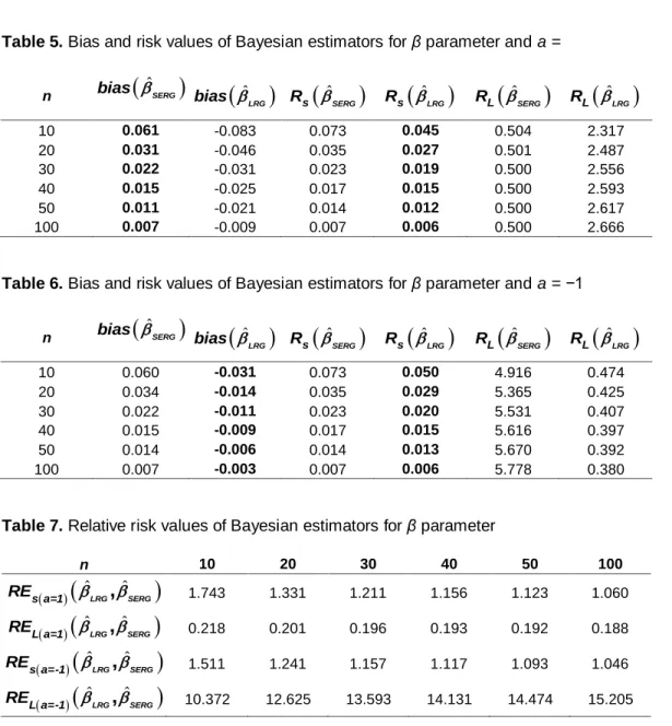
Bias values and risk functions are computed to compare considered Bayesian estimators. A comparison of this type is needed to check whether an estimator is inadmissible under some loss function. Therefore, if it is so, the estimator would not be used for the losses specified by that loss function. For this purpose, the risks of the estimators and the efficiency of them are computed. In each case, a = 1, a = −1, b = 2 and σ = 2 are taken without loss of generality.

Because comparing different loss functions is not reasonable, compare the results in similar loss function, but in different priors. According to results compiled in Tables 2, 3, 5 and 6, all the four considered Bayesian estimators

based on reciprocal gamma prior have small values of bias. Further, the



ˆ_SERG estimator has smaller bias than



ˆ_LRG estimator for a = 1 while



ˆ_LRG estimator has smaller bias than



ˆ_SERG estimator for a = −1.

According to Tables 2, 3, 5 and 6, among the four considered Bayesian risks based SEL the R_S

 

ˆ_LRG has the smallest values of risk for various values of sample size.

Also among the four considered Bayesian risks based LINEX, the R_L

 

ˆ_LJ

has the smallest values of risk for various values of sample size.

Table 2. Bias and risk values of Bayesian estimators for β parameter and a = 1 n



ˆ



SEJ

bias

 

ˆ

LJ

bias R_s



ˆ_SEJ



R_s

 

ˆ_LJ R_L



ˆ_SEJ



R_L

 

ˆ_LJ

10 0.072 -0.090 0.100 0.056 0.047 0.031 20 0.035 -0.047 0.041 0.031 0.020 0.016 30 0.024 -0.031 0.025 0.021 0.012 0.011 40 0.016 -0.025 0.018 0.016 0.009 0.008 50 0.011 -0.022 0.014 0.013 0.007 0.007 100 0.005 -0.011 0.007 0.007 0.003 0.003

Table 3. Bias and risk values of Bayesian estimators for β parameter and a = −1 n bias



ˆ_SEJ



bias

 

ˆLJ





ˆ _SEJ s R Rs

 

ˆLJ RL



ˆSEJ



RL

 

ˆLJ 10 0.065 -0.039 0.099 0.071 0.037 0.032 20 0.034 -0.017 0.041 0.035 0.018 0.016 30 0.022 -0.011 0.025 0.023 0.012 0.011 40 0.018 -0.007 0.018 0.017 0.009 0.008 50 0.013 -0.007 0.014 0.014 0.007 0.007 100 0.007 -0.003 0.007 0.007 0.003 0.003

Table 4. Relative risk values of Bayesian estimators for β parameter

n 10 20 30 40 50 100  



ˆLJ ˆSEJ



s a=1 RE  , 1.524 1.233 1.149 1.110 1.087 1.043  



 ˆLJ ˆSEJ



L a=1 RE , 1.788 1.338 1.214 1.157 1.124 1.060  



ˆLJ ˆSEJ



s a=-1 RE  , 1.164 1.078 1.051 1.038 1.031 1.015  



 ˆLJ ˆSEJ



L a=-1 RE , 1.382 1.174 1.112 1.083 1.066 1.032

Table 5. Bias and risk values of Bayesian estimators for β parameter and a =

n bias



ˆSERG





ˆ



LRG

bias R_s



ˆ_SERG



R_s



ˆ_LRG



R_L



ˆ_SERG



R_L



ˆ_LRG



10 0.061 -0.083 0.073 0.045 0.504 2.317 20 0.031 -0.046 0.035 0.027 0.501 2.487 30 0.022 -0.031 0.023 0.019 0.500 2.556 40 0.015 -0.025 0.017 0.015 0.500 2.593 50 0.011 -0.021 0.014 0.012 0.500 2.617 100 0.007 -0.009 0.007 0.006 0.500 2.666

Table 6. Bias and risk values of Bayesian estimators for β parameter and a = −1

n bias



ˆSERG





ˆ



LRG

bias R_s



ˆ_SERG



R_s



ˆ_LRG



R_L



ˆ_SERG



R_L



ˆ_LRG



10 0.060 -0.031 0.073 0.050 4.916 0.474 20 0.034 -0.014 0.035 0.029 5.365 0.425 30 0.022 -0.011 0.023 0.020 5.531 0.407 40 0.015 -0.009 0.017 0.015 5.616 0.397 50 0.014 -0.006 0.014 0.013 5.670 0.392 100 0.007 -0.003 0.007 0.006 5.778 0.380

Table 7. Relative risk values of Bayesian estimators for β parameter

n 10 20 30 40 50 100  



ˆLRG ˆSERG



s a=1 RE  , 1.743 1.331 1.211 1.156 1.123 1.060  



ˆLRG ˆSERG



L a=1 RE , 0.218 0.201 0.196 0.193 0.192 0.188  



ˆLRG ˆSERG



s a=-1 RE  , 1.511 1.241 1.157 1.117 1.093 1.046  



ˆLRG ˆSERG



L a=-1 RE , 10.372 12.625 13.593 14.131 14.474 15.205

Application to real data

Here, in order to display the usage of proposed model in real data, it is needed to analyze two sets of the seven from the afore presented data in paper by Bennett

and Filliben (2000). Reportedly, they have notified minority electron mobility for

p-type Ga1-xAlxAs with seven different values of mole fraction. To do so, two

data sets are employed relating to the mole fractions of 0.25 and 0.30. The data values are as followed:

Data Set 1 (belongs to mole fraction 0.25): 3.051, 2.779, 2.604, 2.371, 2.214, 2.045, 1.715, 1.525, 1.296, 1.154, 1.016, 0.7948, 0.7007, 0.6292, 0.6175, 0.6449, 0.8881, 1.115, 1.397, 1.506, 1.528.

Data Set 2 (belongs to mole fraction 0.30): 2.658, 2.434, 2.288, 2.092, 1.959, 1.814, 1.530, 1.366, 1.165, 1.041, 0.9198, 0.7241, 0.6403, 0.576, 0.5647, 0.5873, 0.8013, 1.002, 1.250, 1.347, 1.368.

To evaluate the fitting quality of the Rayleigh and LBR distributions, the Kolmogorov-Smirnov (K-S) tests and AIC and BIC’s criterions are used. The

information about comparing both models are given in Table 8. Since probability

values of the LBR model are greater than corresponding values of the Rayleigh model and the AIC and BIC criterions of the LBR model are less than corresponding values of the Rayleigh model. Although the values of considered statistics are not significantly different but we it can be infered that the LBR distribution fits better than the Rayleigh distribution in both considered data.

The MLEs of β are 0.9322 and 0.7309 and the 95 percent confidence

intervals of β based on MLEs as suggested above under heading Parameter

Estimation, can be obtained as (0.6067,1.2577) and (0.4757,0.9861) respectively.

Table 8. Comparing related statistics for Rayleigh and LBR

Data Model D p.value AIC BIC

1 Rayleigh 0.1411 0.7458 46.0090 47.0540

1 LBR 0.1275 0.8427 45.9160 46.9610

2 Rayleigh 0.1354 0.7883 40.3870 41.4320

2 LBR 0.1311 0.8180 39.7820 40.8260

Conclusion

Different estimation procedures were studied for estimating the unknown scale parameter of the WR(α,β) distribution being the maximum likelihood estimator, the method of moment estimator, uniformly minimum variance unbiased estimator, maximum goodness-of-fit estimators and the Bayes estimators. Since it is not possible to compare different methods theoretically, some simulations were used for comparison of different estimators with respect to biases, mean squared errors and risks.

All the four considered Bayesian estimators based on reciprocal gamma prior have small values of bias. In addition, the



ˆ_SERG estimator has smaller bias

than



ˆ_LRG estimator for a = 1 but



ˆ_LRG estimator has smaller bias than



ˆ_SERG estimator for a = −1.

Among the four considered Bayesian risks based SEL the R_S

 

ˆ_LRG has the

smallest values of risk and based LINEX, the R_L

 

ˆ_LJ has the smallest values of risk for various values of sample size. Thus from a Bayesian perspective we suggest using



ˆ_LRG estimator based on SEL and using



ˆ_LJ based on LINEX loss function.

The performance of the MLE and UMVUE is also quite satisfactory and in overall non-Bayesian estimators are better than Bayesian estimators, thereby employing of the MLE and UMVUE estimators can be recommend for all practical purposes.

Acknowledgements

Portions of this paper are developed from the authors’ earlier conference presentation (Ajami & Jahanshahi, 2016).

References

Ajami, M. & Jahanshahi, S. M. A. (2016, August 24-26). Comparison of various estimation methods for size-biased Rayleigh distribution. Paper presented

at the 13th _{Iranian Statistical Conference, Shahid Bahonar University of Kerman,}

Iran.

Alizadeh, N. H. & Arghami, N. R. (2011). Monte Carlo comparison of five exponentiality tests using different entropy estimates. Journal of Statistical

Computation and Simulation, 81(11), 1579–1592. doi:

10.1080/00949655.2010.496368

Bennett, H. S. & Filliben, J. J. A. (2000).A systematic approach for

multidimensional, closed form analytic modeling: minority electron mobilities in

Ga1-xAlxAs heterostructures, Journal of Research of the National Institute of

Standards and Technology, 105(3), 441–452. doi: 10.6028/jres.105.037

Ferguson, T. S. (1996). A Course In Large Sample Theory. New York:

Chapman and Hall.

Gupta, R. C. & Keating, J. P. (1985). Relations for reliability measures

Gupta, R. C. & Kirmani, S. N. U. A. (1990).The role of weighted

distributions in stochastic modeling, Communications in Statistics - Theory and

Methods, 19(9), 3147–3162. doi: 10.1080/03610929008830371

Johnson N. L., Kotz, S., & Balakrishnan, N. (1994). Continuous univariate

distributions, Vol 1 (2nd _{Ed.). New York: Wiley.}

Oluyede, B. O. (1999).On inequalities and selection of experiments for

length-Biased Distributions. Probability in the Engineering and Informational

Sciences, 13(2), 169–185. doi: 10.1017/s0269964899132030

Patil, G. P. & Rao, C. R. (1978).Weighted distributions and size-biased sampling with applications to wildlife populations and human families.

Biometrics,34(2), 179–184. doi: 10.2307/2530008

Patil, G. P. & Ord, J. K. (1976).On size-biased sampling and related

form-invariant weighted distribution. Sankhya: The Indian Journal Of Statistics B, 38,

48–61.

Rayleigh, J. W. S. (1880). On the resultant of a large number of vibrations

of the some pitch and of arbitrary phase, Philosophical Magazine, 5th Series,

10(60), 73–78. doi: 10.1080/14786448008626893

Reshi, J. A., Ahmed, A. & Mir, K. A. (2014). Characterizations and

estimation in the length-biased generalized Rayleigh distribution. Mathematical

Theory and Modeling, 4(6),87-98.

Sanku, D. (2012).Bayesian estimation of the parameter and reliability

function of an inverse Rayleigh distribution, Malaysian Journal of Mathematical

Sciences, 6(1), 113–124.

Soliman, A. A. (2000). Comparison of LINEX and quadratic Bayes

estimators for the Rayleighdistribution. Communications in Statistics - Theory

and Methods, 29(1), 95–107. doi: 10.1080/03610920008832471

Varian, M. M. (1975). A Bayesian approach to real estate assessment. In S.

E. Fienberg and A. Zellner, Ed. Studies in Bayesian Econometrics and Statistics

(In Honor of Leonard J. Savage), pp. 195–208. Amsterdam: North

Holland/Elsevier.

Zelen, M. & Feinleib, M. (1969).On the theory of chronic diseases,

Biometrika, 56(3), 601–614. doi: 10.2307/2334668

Zellner, A. (1986). Bayesian estimation and prediction using loss functions,

Journal of the American Statistical Association. 81(394), 446–451. doi: