Please cite this paper as:
Huang, T., Fildes, R. and Soopramanien, D. The value of competitive information forecasting FMCG retail product sales and the variable selection problem (LUMS Working Paper 2013:1). Lancaster University: The Department of Management Science.
Lancaster University Management School
Working Paper 2013:01
The Value of Competitive Information in
Forecasting FMCG Retail Product Sales and the
Variable Selection Problem
Huang, Tao, Fildes, Robert and Soopramanien, Didier
Lancaster Centre for Forecasting, Department of Management ScienceLancaster University Management School Lancaster LA1 4YX
UK
© Tao Huang, Robert Fildes, and Didier Soopramanien All rights reserved. Short sections of text, not to exceed two paragraphs, may be quoted without explicit permission,
provided that full acknowledgment is given. The LUMS Working Papers series can be accessed at
http://www.lums.lancs.ac.uk/publications
1
The value of competitive information in forecasting FMCG retail product sales and the variable selection problem
Tao Huanga,1 Robert Fildesb Didier Soopramanienc abc
Lancaster Centre for Forecasting, Lancaster University, UK, LA1 4YX
Abstract
Sales forecasting at the UPC level is important for retailers to manage inventory. In this paper, we propose more effective methods to forecast retail UPC sales by incorporating competitive information including prices and promotions. The impact of these competitive marketing activities on the sales of the focal product has been extensively documented. However, competitive information has been surprisingly overlooked by previous studies in forecasting UPC sales, probably because of the high-dimensionality problem associated with the selection of variables. That is, each FMCG product category typically contains a large number of UPCs and is consequently associated with a large number of competitive explanatory variables. Under such a circumstance, time series models can easily become over-fitted and thus generate poor forecasting results.
Our forecasting methods consist of two stages. At the first stage, we refine the competitive information. We identify the most relevant explanatory variables using variable selection methods, or alternatively, pool information across all variables using factor analysis to construct a small number of diffusion indexes. At the second stage, we specify the Autoregressive Distributed Lag (ADL) model following a general to specific modelling strategy with the identified most relevant competitive explanatory variables and the constructed diffusion indexes.
We compare the forecasting performance of our proposed methods with the industrial practice method (benchmark model) and the ADL model specified exclusively with the price and promotion information of the focal product. The results show that our proposed methods generate substantially more accurate forecasts across a range of product categories.
1Corresponding author. Tel.: +44 (0)20 7594 2744. E-mail address: [email protected] (T. Huang),
2 Keywords
Forecasting; Business analytics; OR in marketing; Retailing; Promotions; Competitive information
1. Introduction
Grocery retailers have been struggling with stock-outs for years. Stock-outs cause a direct loss of potential sales and lead to dissatisfied customers. The stock-out of individual items not only has negative impact on its own sales but also on the sales of the whole product category (Kalyanam et al., 2007). Recent studies show that customers whom we once believed to either purchase substitutes or delay purchases when their preferred products are out of stock are actually more likely to switch stores and never come back (Corsten and Gruen, 2003). To avoid the out-of-stock condition, retailers may deliberately increase safety stock (i.e. to over-stock), which substantially reduces profit (Cooper et al., 1999). Under such a circumstance, retailers face a dilemma: they need to balance the loss due to stock-outs and the cost of safety stocks. One of the keys to resolve the cost and service trade-off is to provide accurate forecasts for product sales at the UPC level2 (Corsten and Gruen, 2003). In supply chain management, accurate forecasts are critically important for Just-In-Time (JIT) delivery (Kuo, 2001).
However, forecasting retailer product sales at the UPC level is difficult. Product sales are driven by a large number of factors including price reductions and promotion activities of the focal product (Ali et al., 2009; Blattberg et al., 1995; Christen et al., 1997; Cooper et al., 1999; Gupta, 1988; Lattin and Bucklin, 1989; Mulhern and Leone, 1991), price reductions and promotion activities of competitive products (Demirag et al., 2011; Struse, 1987; Walters, 1991; Walters and Rinne, 1986), various types of advertisement which target specific customer segments (Chandy et al., 2001; Tellis et al., 2000), and product category characteristics (Baltas, 2005; Nijs et al., 2001). Today’s grocery retailers spend a large proportion of their marketing budget on price reductions and promotion activities due to more intense competition (Kamakura and Kang, 2007; Raju, 1995). Price reductions and promotion activities can substantially boost the sales of the focal product, but also cause brand switching and stockpiling, which amplifies the variation of the product sales and makes product sales
2 UPC (Universal Product Code) and SKU (Stock Keeping Unit) are both tracking methods specifying a product
exactly in terms of all of its features such as flavour, colour, and packaging size etc. SKU may however include other elements including the store in which the item is sold. UPC and SKU are used interchangeably in this study as used in the literature.
3
more difficult to forecast (Ailawadi, 2006). The sales of the focal product may also be subject to the negative impact of price reductions and promotion activities of other competitive products exacerbating the forecasting problem (Struse, 1987; Walters, 1991; Walters and Rinne, 1986)
In practice, many retailers use a base-times-lift approach to forecast product sales at the UPC level. Under this approach, retailers initially generate a baseline forecast with simple methods and then make adjustments for any incoming price reduction and promotional event. The adjustments are estimated based on the lift effect of the most recent price reduction and/or promotion, and also the judgements made by brand managers (Fildes et al., 2008). Evidence shows that the forecasting accuracy of this approach is far from satisfactory (Cooper et al., 1999; Fildes et al., 2008). In the recent literature, some studies focus on how the adjustment should be made. For example, a string of studies have tried to help managers with their judgmental decisions for the lift effect (Goodwin, 2002; Lee et al., 2007; Nikolopoulos, 2010). In contrast, Cooper et al. (1999) developed a model-based forecasting system based on promotional events. The system uses a regression style model with a large number of variables related to price, promotions, and store/category specific historical information. Others have proposed time series forecasting models with Taylor (2007) extending an exponential smoothing approach. However, exponential smoothing methods have been criticized for their inability to capture the effects of special events such as promotions, announcements, changes in regulations, and strikes etc. (Lee et al., 2007). In order to capture promotional effects, Kuo (2001), Aburto and Weber (2007) and Ali et al. (2009) all proposed machine learning based approaches which include promotional variables. All apart from Taylor (2007) examined a small number of SKUs however with a limited forecast validation exercise. We discuss the approaches employed in these studies in the next section.
While these studies have incorporated the price and promotion of the focal product in forecasting retailer product sales at the UPC level, they overlooked certain potentially important features of the product market. For example, the time dependence of promotional effects was excluded. Also, the focus of this article, the potential importance of price reductions and promotions of other competitive products was not considered. Past research has established the importance of competitive information on the sales of the focal product (e.g. Dekimpe et al., 1999; Nijs et al., 2001; Van Heerde et al., 2003; Van Heerde et al., 2000). A well-known example is the SCAN*pro model and its extensions which measures
4
cross price elasticity at the brand level (Andrews et al., 2008; Wittink et al., 1988). More recent studies have analysed the cross price elasticity for each individual items and for each store (Wedel and Zhang, 2004). The negative impact of the competitive marketing activities is further divided into the cannibalization effect and the brand switching effect depending on if the impact originates from the products of the same brand or from different brands (Nijs et al., 2001). Some other studies tried to establish a link between the magnitude of the effect of competitive marketing activities, category characteristics, and brand image (Bandyopadhyay, 2009; Blattberg and Wisniewski, 1987; Kamakura and Kang, 2007). However, these studies focus on identifying and estimating the effects of competitive prices and competitive promotions, and they do not consider the operational question facing the retailer of designing models to forecast product sales at the UPC level.
Competitive information has previously been used to forecast product sales at the brand level. For example, Curry et al. (1995) proposed a Bayesian VAR model to forecast product sales at the brand level, and Zhong et al. (2005) extended the model to a Bayesian VECM model which captures the potential co-integration relationship. Divakar et al. (2005) proposed a regression model to forecast beverage sales for manufacturers at the brand level. The regression model contains the price and promotion of the focal product and its main competitors (e.g. Coca versus Pepsi), and it includes varying parameters to take into account the heterogeneity across different distribution channels. While the impact of competitive information is not analysed directly, it does however prove important in specifying a complete model.
These earlier studies do not imply that we can generate more accurate forecasts by including the competitive information at the UPC level. The data at the disaggregate UPC level contains more noise than at the brand level and it is well known that the impacts of competitive prices and competitive promotion are not as strong as the impacts of the price and promotion of the focal product (see Hoch et al., 1995). Thus it is possible for the overall impact of competitive prices and competitive promotion to be submerged in the noise of the data. Moreover, we face a high-dimensionality problem when incorporating competitive information at the UPC level. Today’s grocery retailers typically sell tens of thousands of products and each product category may contain over hundreds of items. Market theory suggests all these items are competing with one another, but it is not possibly to incorporate the competitive information of all these products when forecasting the sales of the focal
5
product. Therefore, in this paper we explore the value of the competitive information in forecasting retailer product sales at the UPC level. The research is significant because unlike most earlier studies it focuses on developing parsimonious econometric models for promotional forecasting using best practice evaluation methods. Methodologically our research offers a novel evaluation of different variable selection approaches in a high dimensionality problem, an issue of theoretical and practical significance in a world of ‘big data’. Besides the theoretical interest, the results have practical significance in that they offer operational guidance to the retail forecaster as to how to produce more accurate forecasts as simply as possible.
The remainder of this paper is organized as follows. In section two, we review previous studies and address their limitations. In section three we explain the high-dimensionality problem when incorporating competitive information. In section four we present our methodology. Section five describes the data. Section six introduces the models. Section seven demonstrates our experimental design. In section eight we present the results. In the last section we draw conclusions on the value of competitive information in UPC retail forecasting, both when the focal product is being promoted and when it is not.
2. Related Literature
Various regression type models have been developed to analyse retailer sales in order to understand the effect of marketing activities at the brand level (Foekens et al., 1992; Foekens et al., 1994). These studies did not directly address the retailer’s forecasting problem associated with operations and stock management because their level of aggregation is too high (i.e. brand rather than UPC) and they exclude any dynamic effects of marketing activities. At the UPC level, perhaps surprisingly given the level of theoretical interest in supply chain planning and the bullwhip effect (Ouyang, 2007; Sodhi and Tang, 2011), there has been very limited empirical work with Rinne and Geurts (1988) considering forecasting performance as a part of an evaluation of promotional profitability. Their model omitted dynamic and competitive effects and offered no evidence on forecasting accuracy. Preston and Mercer (1990) examined a limited number of product categories and again developed static models without competitive effects and with no comparative accuracy evidence.
6
In practice, many retailers use the base-times-lift approach to forecast product sales at the UPC level. The approach generates a baseline forecast and then makes adjustments for any incoming promotional events. Typically, the baseline forecasting model is a variant of exponential smoothing and the adjustment is made judgementally (Fildes et al., 2009). The choice of the baseline is inevitably important and commercial software typically offers users a variety of alternatives. Taylor (2007) applied the quantile exponential smoothing method to generate robust point forecasts for daily supermarket sales. The evaluation was based on comparative error measures (e.g. the average MAE/RMSE relative to exponential smoothing methods), and the model outperformed the benchmark model especially for short horizons. On the other hand, judgmental adjustments are expensive and potentially prone to systematic bias (Fildes et al., 2009; Franses and Legerstee, 2010). An approach to overcome this whilst a multivariate extension of exponential smoothing to monthly supplier data compared to judgmental adjustment has been shown to be effective by Trapero Arenas et al. (2013). A more established approach is due to Cooper et al. (1999) who developed a promotional-event forecasting system which again adopts the “two-step” procedure. The forecasting system first produces a baseline forecast, and then estimates the adjustment but with a more sophisticated model: a regression model with a variety of promotional conditions and store/category specific information as explanatory variables. The regression model was subsequently extended to contain information related to manufacturers and product categories (Cooper and Giuffrida, 2000; Trusov et al., 2006). The forecasting system exhibited superior forecasting performance compared to the base-time-lift approach in terms of the Mean Absolute Error (MAE). However, the regression model is static and the cross-sectional regression model is based on promotional events: thus it ignores the carryover effect of price reductions and promotions and also the time since the last price reduction and/or promotion. Moreover, the system overlooks the impact of competitive prices and competitive promotions on the sales of the focal product.
Some recent studies have tried to forecast product sales at the SKU level using complex time series models to capture promotional effects. Kuo (2001) proposed a fuzzy neural network model to forecast daily milk sales for a convenience store (CVS) franchise company. The neural network model is integrated with a genetic algorithm which learns fuzzy IF±THEN rules for promotions obtained from marketing experts. Their model outperforms conventional simple statistical methods and a single neural network model in terms of the Mean Squared Error (MSE). However, the performance of the models is evaluated with only one single SKU
7
(i.e. 500 cl container of papaya milk.). Aburto and Weber (2007) proposed a hybrid model to forecast SKU sales for a Chilean supermarket. They initially forecast the product sales with a seasonal ARIMA model and then predict the residual of the seasonal ARIMA model using a neural network model with the price and promotional information of the focal product. The hybrid model has better forecasting performance in terms of the Mean Absolute Percentage Error (MAPE) compared to using the SARIMA model and the neural network model separately. The evaluation of the models is also based on only one single SKU (i.e. vegetable oil, 1L). Ali et al. (2009) evaluated the performance of various machine learning algorithms in forecasting retailer sales at the SKU level. The models include the support vector regression (SVR) and the regression tree methods with different priori settings. Their models incorporate the statistics of historical information (i.e. average, sum, trend, standard deviation, etc.) of unit sales and price for the past 4 to 12 weeks, as well as promotion stocks. The forecasting performances of these models are compared in terms of the MAE for non-perishable food products. The SVR model has poor forecasting results. The regression tree method, which has the best forecasting performance overall, outperforms the base-times-lift approach when the focal product is being promoted, but gets outperformed when the focal product in not on promotion. The model in their study ignores the carryover effect of the price and promotion, and also overlooks the impact of competitive promotional activities on the sales of the focal product.
All the studies mentioned above suffer from the problem of: a limited evaluation exercise, too few products, inappropriate errors measures, the failure to use a rolling origin, and a fixed lead time design (Tashman, 2000). As a consequence we remain unsure about both the appropriate econometric specification, and, the relative accuracy of alternative models. These earlier studies by neglecting the dynamics of the market and competitive effects leave unresolved various methodological questions which we now discuss.
3. The high-dimensionality problem
Previous studies have used competitive information to forecast product sales at the brand level (e.g. Curry et al., 1995; Divakar et al., 2005; Foekens et al., 1994). The competitive information typically includes the price and promotion of the main competitive brands. However, it is not straightforward to identify the competitive information at the UPC level. Today’s grocery retailers sell tens of thousands of products purchased from a large number of
8
manufacturers and distributors. A typical product category in the FMCG industry such as Soft Drinks may contain hundreds of items of different flavours, package sizes, and brands. These products are all competitors with each other because they satisfy similar customer needs and wants (Kotler, 1997). Thus when we incorporate competitive information, we face a high-dimensionality problem (Martin and Kolassa, 2009). That is, there are a large number of competitive explanatory variables for possible inclusion in a promotional forecasting model. Time series models can easily get over-fitted and in an extreme case cannot even be estimated because of more explanatory variables than observations. The consequences are poor forecasts.
4. Methodology
In this study, we incorporate competitive information to forecast retailer product sales at the UPC level. To address the associated high-dimensionality problem, we propose a forecasting method that consists of two stages. At the first stage of the method, we refine the competitive information we want to incorporate in the forecasting model. Specifically, we identify the most relevant competitive explanatory variables using variable selection methods (Castle et al., 2008).
The most popular variable selection method is probably the stepwise selection. The method starts with a null model and adds explanatory variables, step-by-step. At each step, the variable with the most significant contribution to the fit of the model is considered for addition while those variables in the model are examined to identify the one with the least significant contribution which is then considered for removal. In each case a threshold is established to determine whether or not the action takes place. The process is complete when no additional actions meet the thresholds.
The stepwise selection method has been heavily criticized for being more likely to retain irrelevant explanatory variables (Flom and Cassell, 2007; Harrell, 2001). Friedman et al. (2001) proposed the Least Absolute Shrinkage and Selection Operator (LASSO) selection procedure. The explanatory variables and the dependent variables are initially standardized to have zero mean values and unit standard deviations. The procedure then estimates a regression model including all the potential explanatory variables but with a constraint for the sum of the absolute values of all the parameter coefficients. That is,
9
∑| |
where
is the vector of observations on the dependent variable is the matrix of the explanatory variables
u is the identically distributed random error is the vector of unknown parameters
N is the number of parameters
is the shrinkage factor which equals to the sum of all the parameter coefficients.
With the constraint, some of the parameter coefficients will tend to be zero, which means that their corresponding explanatory variables will be removed from the regression model. In the selection procedure, the shrinkage factor is determined by an information criterion such as the Akaike Information Criterion (AIC).
Flom and Cassell (2007) compared the performance of LASSO with stepwise selection based using simulation. Their results suggests that stepwise selection tends to miss the relevant explanatory variable when sample size is small and also retain irrelevant explanatory variables, while LASSO has better performance. However, as stated in Efron et al. (2004) variable selection methods may not be able to find a simple model with the most important variables simply because they do not utilize any domain knowledge.
Variable selection methods identify the most relevant competitive explanatory variables and the performance of the resulting forecasting model can relies exclusively on these variables. Alternatively, we can pool information across all the competitive explanatory variables and condense them into a small set of estimated factors at an acceptable cost of information loss (Stock and Watson, 2002a, 2002b). Many studies in the macroeconomics literature used factor analysis to summarize variations among a large set of variables (e.g. Engle and Watson, 1981; Forni and Reichlin, 1996). In particular, Stock and Watson (2002b) constructed a number of factors (named as diffusion indexes) with factor analysis to measure the common movement in a set of macroeconomic variables, and then used them to forecast real economic activities such as price inflation. Their “dynamic factor” model has the following form:
10 where
is an N-dimensional multiple time series of explanatory variables is the matrix with common factors of latent diffusion indexes is the t value of the dependent variable
is a vector of the lagged dependent variable
and are the vectors of the parameter coefficients
and are the errors which are assumed to be and uncorrelated with each other.
In the model, the original competitive explanatory variables, , have been condensed into diffusion indexes at a cost of information loss (i.e. ). Stock and Watson (2002b) found that much of the variation in a large number (>100) of macroeconomic time series (i.e. 39% of the total variation) can be accounted for by only six diffusion indexes. Their proposed models with diffusion indexes outperform the benchmark autoregressive models and VAR models, and they found that the models with the best forecasting performance only contain one or two diffusion indexes.
In this study, we implement both the variable selection method and the principal component analysis at the first stage of the forecasting method. For the variable selection method, we apply both the stepwise selection and the LASSO selection procedure, and we take the explanatory variables selected by the two methods in combination, which limits the possibilities of missing important explanatory variables but at a cost of efficiency. For the principal component analysis, we construct diffusion indexes based on competitive prices and competitive promotions separately, and we choose the most representative factors (e.g. those with eigenvalues substantially larger than others) while keeping the number of factors as small as possible, following the findings by Stock and Watson (2002b)3.
At the second stage, we incorporate the refined competitive information into econometric forecasting models. In this study, we initially construct models with an Autoregressive Distributed Lag (ADL) structure and then simplify the models following a general-to-specific modelling strategy (Hendry, 1995). The general-to-specific modelling strategy starts with a general model assuming that this model properly describes the salient features of the data
3 We choose to retain four diffusion indexes for competitive prices and four diffusion indexes for competitive
promotions. For each product category, the percentages of explained variation in the competitive price data series range from 51% to 79%, and the percentages of explained variation in the competitive promotion data series range from 32% to 69%.
11
generating process. It then simplifies the general model by seeking out valid parsimonious restrictions. The ADL model has the advantage of taking into account the carryover effect of the price and the promotional variables, and with the general-to-specific modelling strategy it is immune to the spurious regression problem. In the literature, the general-to-specific ADL model has exhibited superior forecasting performance in other areas including manufacturer sales, tourism, and air passenger flows (see Albertson and Aylenb, 2003; Fildes et al., 2011; Song and Witt, 2003). The following example shows the general ADL model with the most relevant competitive explanatory variables identified by the stepwise selection and the LASSO selection procedure:
∑ ∑ ∑ ∑ ∑ ∑ ∑ ∑ ∑ ∑ where
is the log sales of the focal product at week
is the log price of the focal product at week
is the promotional index of the focal product at week
is the log price of competitive product at week
is the promotional index of competitive product at week
is the number of competitive price variables selected by the variable selection methods is the number of competitive promotional variables selected by the variable selection methods
is the four-week-dummy variable
is the dummy variable for the calendar event at week . When
, the dummy variable represents the week of the calendar event, and the week before the event if . takes the values from 1 to 9 representing all the calendar events 4
4
The calendar events include Halloween, Thanksgiving, Christmas, New Year’s Day, President’s Day, Easter,
12 are the parameters is the error term and we assume is the order of the lags5
The general ADL model will ideally pass all the misspecification tests (e.g. the F-test, the Breusch-Godfrey test for autocorrelation, and tests for heteroskedasticity and normality). The model may be estimated by OLS with the usual interpretations of the statistics whether or not the data series are stationary, because sufficient lags were included to remove any autocorrelation (although with some potential loss of efficiency) (Song and Witt, 2003). A well-specified ADL model can then be simplified following the general-to-specific strategy. For example, we first estimate the general ADL model and remove the explanatory variable with the highest p-value for the parameter restriction test. We then estimate the reduced model and re-conduct all the misspecification tests. If the reduced model passes all these tests, we move on to remove the variable with the highest p-value in the new estimation, provided that the previous variable has already been removed, and so forth. Otherwise we will add the variable back and repeat the process by removing the variable with the second highest p -value for the parameter restriction test. In the modelling process we remove the variables with incorrect signs. We also remove the explanatory variables which are not economically significant (i.e. with very small parameter coefficients) to achieve parsimony. The final simplified ADL model must pass all the misspecification tests which are passed by the general ADL model. The model is estimated by OLS with robust estimators in the presence of heteroscedasticity. The following example shows the general-to-specific ADL model with the diffusion indexes:
5
In the preliminary analysis, L is initially set as two. If the general model does not pass the misspecification tests, more lags of the price, promotion, and sales variables are added to the general model. In our modelling, for most UPCs, the ADL models do not contain more than two lags of these variables.
13 ∑ ∑ ∑ ∑ ∑ ∑ ∑ ∑ ∑ ∑ where
is the diffusion index of competitive prices at week .
is the diffusion index of competitive promotion at week .
P and Q are the number of initially retained diffusion indexes, and
5. The data
In this study we use the weekly data from Dominick’s Finer Foods, a large U.S. retail chain in the Chicago area. The data is publicly available from the University of Chicago website6. An advantage of using this dataset is that a large number of studies have been conducted based on this dataset and many of them focus on identifying and measuring the effectiveness of the marketing mix activities (e.g. Fok et al., 2006; Kamakura and Kang, 2007; Song and Chintagunta, 2006). However, perhaps surprisingly given the importance of forecasting at the UPC level, none of the studies using this dataset focuses on evaluating the performance of forecasting models. The dataset contains product information at the UPC level including unit sales, price, and promotions for 399 weeks. There are three different types of promotions: “Simple price reduction”, “Bonus buy”, and “Coupons”. “Bonus buy” is the dominant type,
which corresponds to over 75% of the all the promotional events; 24.5% of promotions are “Simple price reduction”; only less than 0.5% of promotions are “Coupons”. In this study, we
use one single variable to represent the presence of all the promotional activities. We aggregate the data across 83 stores using constant weights based on the percentage of All Commodity Volume (ACV) of each store (see Hoch et al., 1995; Pauwels and Srinivasan,
14
2004)7. In this study, we conduct our evaluation based on 122 products from 6 diverse product categories including Bottled Juice, Soft Drinks, Bath Soap, Front-End-Candies, Frozen Juice, and Bathroom Tissue8.
Table 1 Characteristics of the data series for the products in each category
Product category Selected UPCs Promotional intensity Promotional index Lift effect Std/Mean ratio of sales Std/Mean ratio of price Bottled juice 34 0.21 (0.09) 0.78 (0.05) 169% 0.76 0.53 Soft drinks 20 0.27 (0.09) 0.78 (0.12) 812% 1.63 0.86 Bath Soap 20 0.13 (0.04) 0.55 (0.09) 113% 0.44 0.62 Front-End-Candies 15 0.14 (0.13) 0.84 (0.05) 57% 0.40 0.23 Frozen Juices 15 0.22 (0.11) 0.80 (0.10) 187% 0.88 0.75 Bathroom Tissues 18 0.30 (0.09) 0.82 (0.05) 335% 1.26 1.49
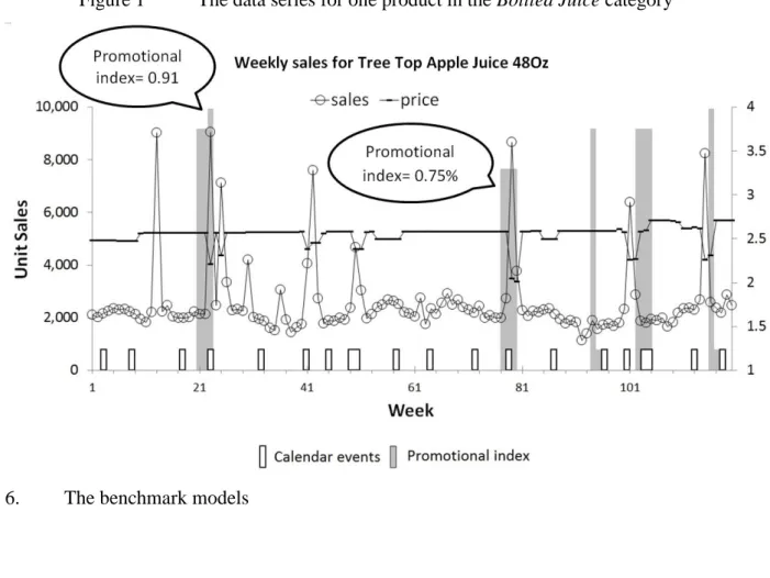
In Table 1 we summarize the characteristics of the data series for the 122 products during a time period of 200 weeks. First, it summarizes the promotional intensity. For example, we choose 34 products from the Bottled Juice category. On average, these 34 products are being sold on promotion for 42 weeks during the 200 weeks (i.e. an intensity of 0.21, with a standard deviation of 0.09). Second, it summarizes the average promotional index value. For example, the average promotional index value for the Bottled Juice category is as high as 0.78 (with a standard deviation of 0.05), which indicates that the products in this category tend to be promoted simultaneously across all the selected stores. Third, Table 1 summarizes the lift effect of the promotions. Take the Bottle Juice category as an example, the promotions in this category increase the sales of focal product by 169% on average compared to the baseline predicted sales assuming there were no promotion. Finally, Table 1 exhibits the average ratio of standard deviation versus mean for both sales and price of the products in
7 Our study is based on 83 stores because some other stores have limited historical data; All Commodity
Volume (ACV) is the total annual revenue (i.e. the U.S Dollar, in this context) of the store. Notice that the ACV is calculated based on the products of the entire store, rather than the products of a specific category. For example, suppose a product is being sold on 3 dollars with promotion in a store and the ACV of the store is 100 million dollars, and it is being sold on 2 dollars without promotion in another store with an ACV of 10 million dollars. The aggregated price would be 3*(100/110)+ 2*(10/110)= 2.91 dollar, and the promotional index would be 1*(100/110)+ 0*(10/110)=0.91. In our study, as pointed out by Hoch et al. (1995), the retailer tends to adopt a uniform pricing strategy where they increase or decrease the price for all the stores at the same time.
15
each category. Among these product categories, Bath Soap and Front-end-Candies have the least variations for their product sales and price, and they also have the least intensive promotions. In contrast, Soft Drinks and Bathroom Tissues are heavily promoted and exhibit highly variations for the sales and price of their products. Therefore, our study covers data of a wide range of sales and promotional conditions.
Figure 1 is an example for one product in the Bottled Juice category (i.e. Tree Top Apple Juice 48Oz). The figure exhibits its unit sales, price (in U.S dollar), calendar events, and promotional periods which are highlighted in darker bars. The length of the darker bars indicates the value of the promotional index which is between 0 and 1. The price and promotional index are both aggregated across multiple stores based on the percentage of ACV of each store. We applied the Augmented Dickey–Fuller test to investigate the stationarity of these data series for all the data series of the 122 products, and we find that most data series are stationary9.
Figure 1 The data series for one product in the Bottled Juice category
6. The benchmark models
9 We find 110 out of 122 data series for unit sales, 106 out of 122 data series for price, and all the data series for
16
In this study we consider two basic benchmark models: 1) the robust simple exponential smoothing (SES) model which focuses exclusively on the pattern of previous product sales; 2) the industrial base-times-lift approach which first produces baseline forecasts and then makes adjustments for any incoming promotional event. In practice, the adjustment of the base-times-lift approach is either determined by estimates from historical data or managers’ judgement. In this study, we approximate the former following Ali et al. (2009):
{
where is the baseline forecast for week generated by a simple exponential smoothing model. is the actual sales value in the previous week when the focal product was not on
promotion. is the parameter which is estimated by minimizing the mean squared error in the estimation period. The adjustment is calculated as the increased sales from the most recent promotion of the focal product. In this study, we use aggregated data across multiple stores, thus the effects of promotions are represented by promotional indexes instead of promotional dummies. For example, if the most recent promotion has a promotional index value of 0.6 and we consider the “lift” effect as L. Then the adjustment for the forthcoming promotion with an index value of 0.9 will be (0.9/0.6)* L = 1.5L.
In this study we propose two forecasting methods which both capture the effect of competitive information but in distinct ways. The first method is the general-to-specific ADL model with the most relevant competitive explanatory variables identified by the variable selection methods (i.e. the ADL model). The second is the general-to-specific ADL model with the diffusion indexes constructed using factor analysis (i.e. the ADL-DI model). We include the competitive price and promotion variables for most products of each product category10. To understand the value of the competitive information, we also include the general-to-specific ADL model which is constructed exclusively with the price and promotional information of the focal product (i.e. the ADL-own model).
7. Experimental design
10
We implement the variable selection methods and the principal component analysis based on the price and promotional variables of a total number of 307 competitive products including the focal 122 products. We try to include as many products as possible provided their data are available.
17
All the studies we have identified which forecast product sales were conducted with a single fixed forecasting origins (e.g.Ali et al., 2009; Cooper et al., 1999; Divakar et al., 2005). However, evaluation results based on single forecast origins can be unreliable when the forecasting results are sensitive to both randomness and possible systematic business cycle effects (Fildes, 1992). In this study, we evaluate the performance of our models with 70 rolling forecast origins, which partially controls for the effect of any specific effects arising from a particular origin. Forecast horizon should also be fixed in any forecast comparisons. We first estimate the models with a moving window of 120 weeks and forecast one to weeks ahead. The forecast horizons were chosen to take into account typical ordering and planning periods, and we set to be 1, 4, and 12. We then move the estimation window forward week by week throughout the remaining sample period and we re-estimate the models based on the updated data sets. Finally we have 70 sets of one to weeks ahead forecast. We generate forecasts using the actual value of the explanatory variables and the forecasted values of the lagged dependent variables when the lead times are greater than one. The promotional variables are usually known to the retailer as they form part of an agreed promotional plan with suppliers. We specify the ADL models with the data from week 1 to week 200, which represents the model that would ideally be selected based on a foreknowledge of the data (Fildes et al., 2011). Alternatively, the models can be re-specified for each rolling event based on each the moving estimation window.
We evaluate the forecasting performance of the various models using five error measures: the MAE, the Mean Absolute Scaled Error (MASE), the MAPE, the symmetric Mean Absolute Percentage Error (sMAPE), and the Average Relative Mean Absolute Error (AvgRelMAE). The MAE has been widely used in practice but has been criticized for its limitation of being scale dependent. For example, suppose that a model has good forecasting performance for one product category with large sales volumes but poor forecasting performance for another product category with smaller sales volumes. If we compare the results across the two product categories, the results for the product category with large sales volumes would dominate the overall results, and we would be misguided to believe that the model has universal good forecasting performance (Chatfield, 1988). In this study, the MAE for data series calculated with forecast horizon for the rolling event is:
∑| ̂ |
18
where is the actual value in the forecast period for data series based on the rolling event, and ̂ is the forecast value for data series based on the rolling event11.
The MASE was proposed by Hyndman and Koehler (2006). It can be considered as a “weighted” arithmetic mean of the MAE based on the variations of the sales data in the estimation period. The MASE calculated across data series with forecast horizon for the
rolling event is:
∑(| |)
∑
where in the equation of , the numerator, , is the MAE for data series calculated with forecast horizon for the rolling event. The denominator is the sum of one-step-ahead errors by a no change naïve model in the estimation period. is the
actual value of data series in the estimation period for the rolling event, and is the
total number of observations in the estimation period. The MASE has good properties such as being robust to zero actual values and scale independent, but it puts more weights to the data series which are comparatively stable (e.g. given the same MAE, will be extremely large if the no change naïve model generates very small errors), which makes it vulnerable to outliers.
The MAPE is the error measure most widely used in practice (Fildes and Goodwin, 2007). It penalizes the forecasts above actual values more heavily than the forecasts below actual values (Armstrong and Collopy, 1992). The sMAPE was proposed to overcome this disadvantage (Makridakis, 1993). The two error measures calculated for data series s with forecast horizon for the rolling event are shown as follows:
11 Note that, in this study, although our econometric models are based on log sales, we calculate all the error
19 ∑ | ̂ | ∑ | ̂ ̂ |
However, both percentage error measures including the MAPE and the sMAPE can be distorting when the actual values and the forecast values are relatively small compared to the forecast error, in which case the resulting percentage errors become extremely large (Hyndman and Koehler, 2006). The sales at the UPC level exhibit high degree of variations due to seasonal effects, changing stages of product life cycle, and particularly promotional activities. Under such a circumstance, it is very likely to have large forecast errors associated with relatively low product sales, which makes the percentage based error measures less advisable in our context (Davydenko and Fildes, 2013).
The four error measures are all approximations of the unknown loss function of the retailer, and they penalize the forecast errors from different perspectives. To make a fair comparison, we assess the overall forecasting performance of the candidate models by calculating the mean value of all the four error measures across rolling events and data series considering different forecasting horizons :
∑ ∑ ∑ ∑ ∑ ∑ ∑
where , , , and are the error measures calculated across data series and rolling events based on forecast horizon (i.e. , , and =1, 4 and 12). We can test the statistical significance for the difference between the
20
forecasting results of the various models using the Wilcoxon signed rank (SR) test. The Wilcoxon SR test can be considered as a non-parametric version of a paired sample t-test but does not assume the errors follow any specific distribution.
Considering the limitations of the four error measures, Davydenko and Fildes (2013) recommended the AvgRelMAE, which is a geometric mean of the ratio of the MAE between the candidate model and the benchmark model. In this study, we take an average of the AvgRelMAE across all the rolling events (i.e. ) and data series with respect to forecast horizon :
∑ (∏ ) ∑
where is the MAE of the candidate model for data series calculated with forecast horizon for the rolling event and is the MAE of the benchmark model for data series calculated with forecast horizon for the rolling event. is the AvgRelMAE calculated across data series and rolling events with respect to forecast horizon (i.e. , , and =1, 4 and 12). The AvgRelMAE has the advantages of being scale independent and robust to outliers, also with more straightforward interpretation: a value smaller than one indicates an improvement by the candidate model.
8. Results
We investigate the models’ relative forecasting performance under conditions of two dimensions which may influence the outcome: 1) different forecast horizons; 2) whether the focal product is being promoted. Earlier research by Ali et al. (2009) compares the forecasting performance of different methods for the promoted forecast periods and non-promoted forecast periods separately. Their regression tree model beat the base-times-lift benchmark model when the focal product is being promoted but is outperformed by the benchmark model when the focal product is not on promotion. Their explanation is that the sales of the focal product are relatively stable when the focal product is not on promotion, and this stability would benefit simple models such as the exponential smoothing method. This explanation neglects the fact that, even during the periods when the focal product is not
21
being promoted, its sales could also be driven by promotions of other competitive products. In this study, we therefore divided the forecast period as promoted period and non-promoted period.
Table 2 The models’ forecasting accuracy and rankings: averaged over forecast horizons from one to twelve weeks (122 UPCs)
Model MAE Rank MASE Rank SMAPE Rank MAPE Rank
Whole forecast period
SES 1984 5 0.93 5 42.30% 5 66.40% 5
Base-times-lift 1498 4 0.81 4 32.70% 4 32.00% 3
ADL 969 1 0.64 2 23.80% 2 28.40% 2
ADL- own 1079 3 0.67 3 25.60% 3 32.50% 3
ADL-DI 992 2 0.63 1 23.00% 1 27.30% 1
Promoted forecast period
SES 2949 4 1.78 4 49.10% 4 47.50% 5
Base-times-lift 3149 5 1.81 5 55.10% 5 41.70% 4
ADL 1875 1 1.19 2 28.10% 2 31.80% 2
ADL- own 2031 3 1.2 2 29.10% 2 34.90% 3
ADL-DI 1969 2 1.16 1 27.30% 1 31.50% 1
Non-promoted forecast period
SES 1423 5 0.72 5 42.30% 5 81.30% 5
Base-times-lift 390 2 0.5 3 22.30% 2 27.80% 2
ADL 369 2 0.47 2 21.70% 2 26.20% 2
ADL- own 463 4 0.49 3 24.10% 4 31.10% 4
ADL-DI 330 1 0.45 1 20.60% 1 24.30% 1
Table 2 exhibits the forecasting accuracy of the various models averaged over horizons from one to twelve weeks based on the various absolute error measures as well as the rank of each model. Note that some models will have the same rank if their performances are not significantly different from each other according to the Wilcoxon sign rank test12. For the whole forecast period, the base-times-lift approach has better performance compared to the SES method. These two benchmark models are both significantly outperformed by the
22
own model for all the error measures, which suggests that the ADL model captures the effects of the price and the promotional activities more effectively than the base-times-lift approach. The ADL model and the ADL-DI model both incorporate the competitive information and they significantly outperform the ADL-own model for all the error measures.
Table 2 also shows the forecasting performance of the various models for the promoted forecast period. The SES method and the base-times-lift approach are significantly outperformed by the ADL-own model, which is consistent with the result for the whole forecast period. However, the ADL model no longer outperforms the ADL-own model significantly when ranked by the MASE and the sMAPE. There are two possible reasons. First, the impact of the promotional activities of the focal product is substantially larger than the impact of the competitive promotion activities (Hoch et al., 1995). Thus the impact of the competitive promotion activities may become submerged in the impact of the promotional activities of the focal product. Second, retailers benefit from the sales of the whole product category rather than individual brands or UPCs, and they tend to avoid simultaneously promoting the product and its main competitors, which will not necessarily increase store sales (e.g. a large proportion of the sales increase come from brand switching) but definitely lower the profit margin (Gupta, 1988; Van Heerde et al., 2003). As a result, when the focal product is being promoted, the competitive information missed by the ADL-own model tends to become less valuable and the ADL model will tend to generate similar forecasts with the ADL-own model. However, the ADL-DI model significantly outperforms the ADL-own model for all error measures even for the promoted period. One explanation is that the diffusion indexes used in the ADL-DI model incorporates competitive information not only from the most relevant competitive explanatory variables but also by pooling across all the competitive explanatory variables.
In Table 2, for the non-promoted forecast period, again the SES method has the poorest forecasting result, but the base-times-lift approach has very good forecasting performance- it significantly outperforms the ADL-own model for all the error measures expect for the MASE. This is consistent with the findings by Ali et al. (2009) that when the focal product is not on promotion, the base-times-lift approach can be hard to beat. Essentially it uses only the data from the non-promoted periods to calculate the smoothing forecast, removing the promotional peaks. The ADL model outperforms the base-times-lift approach for the MASE
23
but has comparable performance for all the other error measures. However, the ADL-DI model still significantly outperforms the base-times-lift approach for all the error measures.
Table 3 The models’ forecasting accuracy and rankings: with one week ahead forecast horizon (122 UPCs)
.
Model MAE Rank MASE Rank SMAPE Rank MAPE Rank
Whole forecast period
SES 1980 5 0.79 5 39.10% 5 60.70% 5
Base-times-lift 1456 4 0.69 4 29.00% 4 26.70% 4
ADL 928 1 0.53 2 20.60% 2 23.30% 2
ADL- own 991 3 0.53 2 21.00% 3 24.40% 3
ADL-DI 941 2 0.52 1 19.90% 1 22.60% 1
Promoted forecast period
SES 3036 4 1.56 4 45.90% 4 44.90% 5
Base-times-lift 3159 5 1.67 5 52.40% 5 39.10% 4
ADL 1860 1 1.00 1 25.50% 2 28.10% 2
ADL- own 1967 3 0.99 1 25.10% 2 29.00% 2
ADL-DI 1921 2 0.98 1 24.30% 1 27.80% 1
Non-promoted forecast period
SES 1363 5 0.59 5 38.60% 5 73.00% 5
Base-times-lift 345 3 0.39 4 18.50% 2 21.50% 2
ADL 320 2 0.36 2 18.10% 2 20.50% 2
ADL- own 361 3 0.36 2 19.00% 2 22.00% 2
ADL-DI 293 1 0.35 1 17.40% 1 19.20% 1
Table 4 The models’ forecasting accuracy and rankings: averaged over forecast horizons from one to four weeks (122 UPCs)
.
Model MAE Rank MASE Rank SMAPE Rank MAPE Rank
24 SES 1963 5 0.84 5 40.00% 5 61.80% 5 Base-times-lift 1474 4 0.72 4 30.30% 4 28.50% 3 ADL 955 1 0.58 2 22.30% 2 25.70% 2 ADL- own 1033 3 0.58 2 23.10% 3 27.70% 3 ADL-DI 969 2 0.57 1 21.30% 1 24.60% 1
Promoted forecast period
SES 2984 4 1.67 4 47.20% 4 46.30% 5
Base-times-lift 3150 5 1.71 5 53.60% 5 40.50% 4
ADL 1873 1 1.12 2 27.10% 2 30.30% 2
ADL- own 1986 3 1.09 2 27.20% 2 31.90% 2
ADL-DI 1948 2 1.07 1 25.90% 1 29.80% 1
Non-promoted forecast period
SES 1364 5 0.64 5 39.80% 5 74.70% 5
Base-times-lift 369 2 0.42 2 19.80% 2 23.50% 2
ADL 349 2 0.41 2 19.90% 2 23.10% 2
ADL- own 414 4 0.42 2 21.40% 4 25.60% 4
ADL-DI 314 1 0.39 1 18.80% 1 21.30% 1
Table 3 and Table 4 show the forecasting performance of the various models for different forecast horizons. The results are in consistent with the results we observe for the one to twelve-weeks-ahead forecast horizon.
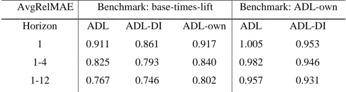
We also calculate the relative error measures proposed by Davydenko and Fildes (2013). Table 5 shows the AvgRelMAE of various candidate models for different forecast horizons. When we compare the candidate models to the benchmark base-times-lift approach, the values are all smaller than 1, which indicates that the ADL model, the ADL-DI model, and the ADL-own model all outperform the benchmark base-times-lift model. In addition, the improvements by these models become more substantial as the forecast horizon increases. For example, the AvgRelMAE for the ADL-DI model decrease from 0.861 to 0.746 as the forecast horizon increase from one week to one-to-twelve weeks. Table 5 also calculates the AvgRelMAE of the candidate models compared to the ADL-own model. The values for the ADL-DI model are all smaller than 1, which indicates that the ADL-DI model outperforms the ADL-own model for all forecast horizons. Again we see the improvements become more
25
substantial as the forecast horizon increases (from 0.953 to 0.931). The values for the ADL model are all smaller than 1 except for one week forecast horizon (i.e. the value is 1.005), which indicates the ADL model is outperformed by the ADL-own model for the one-week-ahead forecast horizon, although only slightly. However, as the forecast horizon increases, the value of AvgRelMAE for the ADL model decreases below 1 (e.g. 0.982 and 0.957), which suggests that it has superior forecasting performance than the ADL-own model which just relies on the price and promotional information of the focal product.
Table 5 The AvgRelMAE of the candidate models for different forecast horizons
AvgRelMAE Benchmark: base-times-lift Benchmark: ADL-own
Horizon ADL ADL-DI ADL-own ADL ADL-DI
1 0.911 0.861 0.917 1.005 0.953
1-4 0.825 0.793 0.840 0.982 0.946
1-12 0.767 0.746 0.802 0.957 0.931
9. Conclusions and future research
Today one of the main concerns of grocery retailers is to reduce stock-outs while controlling the safety stock level. Stock-outs directly lead to profit loss and also dissatisfied customers. One of the keys to overcome this tension relies on more accurate forecasts.
In practice, many retailers use the base-times-lift approach to forecast product sales at the UPC level. The approach is based on a simple method and takes into account the effect of promotions in an ad hoc way. In the literature, studies have proposed sophisticated data mining models and machine learning algorithms, trying to capture the effect of promotions more effectively (Ali et al., 2009; Cooper et al., 1999). However, these methods have several limitations. For example, they ignore the carryover effect of promotions and overlook the effect of competitive information. These models are also too complex and difficult to interpret. They rely on expertise that may well not be available and the company instead substitutes judgment for more formal modelling efforts (Fildes and Goodwin, 2007).
26
In this paper, we investigate the value of the promotional information including competitive price and competitive promotional variables in forecasting retailer product sales at the UPC level. We propose a forecasting method of two stages. At the first stage, we deal with the high-dimensionality problem associated with the retail data at the UPC level using two distinct methodologies. First we identify the most relevant competitive explanatory variables with two variable selection methods in combination (i.e. the stepwise selection and the LASSO procedure). Alternatively we pool information across all the competitive variables and condense them into a handful number of diffusion indexes at the cost of some information loss, based on factor analysis. At the second stage, we incorporate the identified most relevant competitive explanatory variables and the constructed diffusion indexes into the Autoregressive Distributed Lag (ADL) model following a general-to-specific modelling strategy. The general ADL model captures the carryover effect of price and promotions, and the general-to-specific modelling strategy ensures the parsimony and data congruence of the model. The model also benefits from good interpretability. For example, managers can make inference about how the sales of the focal product are driven by marketing activities of the focal product and other competitive products.
Both the ADL model and the ADL-DI we propose in this study significantly outperform the two basic benchmark models and the ADL-own model which is construct exclusively with the price and promotion information of the focal product, and the improvements in forecasting accuracy become more substantial as the forecast horizon increases, which proves the value of the competitive information in forecasting retailer product sales at the UPC level. We have also investigated the forecasting performance of the models considering whether or not the focal product is being promoted. For the promoted forecast period, the ADL-DI model significantly outperforms the benchmark models and the ADL-own model, while the ADL model significantly outperforms the benchmark models but has comparable forecasting performance with ADL-own model. For the non-promoted period, although simple methods are hard to beat when product sales are relatively stable, the ADL-DI model significantly outperforms the benchmark models and the ADL-own model for all the error measures and for all the forecast horizons. The ADL model also significantly outperforms the ADL-own model and the SES model, although has comparable forecasting performance with the base-times-lift approach.
27
There remains the potential to improve the forecasting model. One way is to identify the competitive products more effectively. For example, we have included most products within each product category when implementing the variable selection methods and the factor analysis, and the uncertainty could potentially be reduced if a “short list” of the main competitors for each item can be constructed based on the market knowledge of category managers (Dekimpe and Hanssens, 2000). Also in this study we do not take into account the effect of advertising. Thus one possible way to improve the forecasting accuracy is to incorporate advertising information, although previous studies found the effect of advertising temporary and fragile (Chandy et al., 2001). Datasets such as this may also contain evidence on the different types of promotions such as simple price reduction, bonus buy, and coupon, and it may be possible to distinguish between them. However, this would substantially increase the number of competitive explanatory variables, which adds more uncertainty to the selection of competitive explanatory variables and the construction of diffusion indexes. An additional possible way to improve the model is to further incorporate information from other substitutive and complementary product categories (Bandyopadhyay, 2009; Kamakura and Kang, 2007; Song and Chintagunta, 2006). Again the effect would be to increase the size of the variable set dramatically and demand even more of the practitioner.
Two other modelling issues might merit further work, an examination of the exogeneity of the promotional variables (though this would be unlikely to lead to forecast improvements) and the use of Bayesian estimation methods, an approach which has the merit of permitting a more disaggregate approach. This study was carried out using weekly aggregate data (across stores). While such forecasts are needed for ordering and distribution decision making, store-level forecasts on a daily basis are also needed. They can of course be derived from simple proportionate disaggregation processes, an approach often used in practice, but it is an open research question as to whether daily explicit model-based disaggregate forecasts are to be preferred.
In this study, we constructed the general-to-specific ADL model manually. The modelling process is subjective and relies overmuch on our tacit knowledge of modelling specification. Alternatively, Hendry and Krolzig (2001) proposed the PcGive software which automatically constructs the model. The software starts with a general model and simplifies the model exclusively based on diagnostic tests. However, the software does not incorporate marketing theory and Fildes et al. (2011) found that the ADL model built manually by the model builder
28
outperformed the one constructed by the PcGive software. In preliminary work here the automatic approach also did not prove effective.
The industry standard benchmark method proved of limited value for capturing promotional effects. This paper shows that for practical purposes the company forecaster could achieve superior forecasting performance by incorporating competitive information, either through variable selection methods or factor analysis, with the ADL model built manually following the general-to-specific strategy. Although the development of an automatic ADL model proved costly in terms of forecasting accuracy, and we see this as difficult to implement for most organizations without the support of expert staff (Montgomery, 2005), the benefits of embracing a more sophisticated model building approach have proved substantial (e.g. the ADL-DI model has reduced the sMAPE by around 30% compared to the bases-times-lift model for the one-to-twelve weeks forecast horizon) and if implemented should lead to substantial savings in the distribution chain.
Reference
Aburto, L., & Weber, R. (2007). Improved supply chain management based on hybrid demand forecasts. Applied Soft Computing, 7, 136-144.
Ailawadi, K. L. (2006). Promotion Profitability for a Retailer: The Role of Promotion, Brand, Category, and Store Characteristics. Journal of marketing research, XLIII, 518-535.
Albertson, K., & Aylenb, J. (2003). Forecasting the behaviour of manufacturing inventory
International Journal of Forecasting, 19, 299-311.
Ali, Ö. G., SayIn, S., van Woensel, T., & Fransoo, J. (2009). SKU demand forecasting in the presence of promotions. Expert Systems with Applications, 36.
Andrews, R. L., Currim, I. S., Leeflang, P., & Lim, J. (2008). Estimating the SCAN*PRO model of store sales: HB, FM or just OLS? international Journal of research in marketing, 25, 22-33. Armstrong, J. S., & Collopy, F. (1992). Error measures for generalizing about forecasting methods:
Empirical comparisons. International Journal of Forecasting, 8, 69-80.
Baltas, G. (2005). Modelling category demand in retail chains. Journal of The Operational Research Society, 56, 1258-1264.
Bandyopadhyay, S. (2009). A Dynamic Model of Cross-Category Competition: Theory, Tests and Applications. Journal of Retailing, 85, 468-479.
Blattberg, R. C., Briesch, R., & Fox, E. J. (1995). How promotions work? Marketing Science, 14. Blattberg, R. C., & Wisniewski, K. J. (1987). How Retail Price Promotions Work: Empirical Results.
Working Paper 43, University of Chicago, Chicago IL.
Castle, J. L., Doornik, J. A., & Hendry, D. F. (2008). Model Selection when there are Multiple Breaks.
Working paper No. 407, Economics Department, University of Oxford.
Chandy, R. K., Tellis, G. J., MacInnis, D. J., & Thaivanich, P. (2001). What to Say When: Advertising Appeals in Evolving Markets. Journal of Marketing Research, 38, 399-414.
Chatfield, C. (1988). Apples, oranges and mean square error. International Journal of Forecasting, 4, 515-518.
Christen, M., Gupta, S., Porter, J. C., Staelin, R., & Wittink, D. R. (1997). Using market level data to understand promotion effects in a nonlinear model. Journal of marketing research, 34.