The Dynamic Steady State of an Electrochemically Generated Nanobubble

Supporting Information. Part 1

The Dynamic Steady State of an Electrochemically Generated Nanobubble

Yuwen Liu†, ‡_{, Martin A. Edwards}†_{, Sean R. German}†_{, Qianjin Chen}† _{and Henry S. White}†

†_{Department of Chemistry, University of Utah, Salt Lake City, UT 84112, United States} ‡ _{College of Chemistry and Molecular Sciences, Wuhan University, Wuhan, 430072, China}

S1. Description of Simulations

A geometry with axial symmetry was used in all simulations in the present study. It is assumed that bubble dissolution is limited by diffusion and that the dissolved gas concentration at the bubble interface is always at equilibrium with the bubble’s internal pressure (determined by its radius of curvature) as described by Henry’s law (Eq. SI1). The internal pressure obeys the Young–Laplace equation (Eq. SI2). The electrode reaction 2H+ _{+ 2e}-→ _H

2 is assumed to be diffusion limited, which is reflected by zero concentration of H+ at the exposed

Pt. In the following, we give a detailed description of simulations of a single H2 nanobubble in presence of

electrode reactions.

Henry’s law is given by,

s H in

C =K p (SI1)

where

K

Young–Laplace equation is used to define the internal pressure (pin):

in ex nb 2 / sin p p r γ θ = + (SI2)

where γ is the surface tension of gas/solution interface, rnb is the pinned radius of the nanobubble, θ is the inner

contact angle, and pex is the external pressure (atmospheric pressure).

The 2D axisymmetric geometries of a nanobubble pinned on a nanodisk electrode shrouded in glass and at a recessed disk nanoelectrode are shown schematically in Figure SI1 (a) and (b), respectively. Note, these geometries are not drawn to scale. In particular, the radius of the large quadrant defined by boundary ⑤ was set at 1000 a, where a is the radius of the Pt disk nanoelectrode. The different colors represent the different boundary conditions (see below), with the red line (boundary ④) representing the axis of symmetry.

(a) (b)

Figure SI1. The 2D axisymmetric geometry of single nanobubble (a) on adisk nanoelectrode coplanar with a glass support, and (b) at a recessed disk nanoelectrode (both not to scale). Yellow line (①): the electrode surface; green line (②): glass surface; blue line (③): bubble-electrolyte interface; red line (④): the symmetry axis, black line (⑤): bulk solution far away from the bubble surface.

Fick's second law is used as domain equation to describe the steady-state transport rate of both H2 and H+,

2 2 2 2 1 ( ) 0 i i i i i i c c c c J D t r r r z ∂ _{= −∇ ⋅ =} ∂ ₊ ∂ ₊∂ ₌ ∂ ∂ ∂ ∂ (SI3)

where

c

J

D

As we were looking for steady-state solutions, the left-hand side of this equation is set to zero, meaning there is no change in concentration with time. The diffusion flux of the species i is defined by Fick’s first law as,

i i i

J = − ∇D c (SI4)

where i = H2 or H+.

The boundary conditions are as follows:

In the experiments, the electrode potential is set at E ≫ Eo _(H+_/H

2) such that the reaction is mass transport

+ H

0

c

=

As neither species is transported into or out of the surface of glass (boundary ② in Fig. SI1) there is no normal flux, which is described by:

0 = ⋅J_i

n (SI6)

where i = H2 or H+, and n represents the inward pointing unit normal to the surface.

At the bubble-solution interface, (boundary ③ in Fig. SI1) we assume that there is no kinetic hindrance to gas transport and so the surface concentration of H2 can be described by Henry’s law (Eq. SI1). The internal

pressure is defined by Young–Laplace equation (Eq. SI2). The curvature radius of the nanobubble (rc) is given

by,

r

=

r

/ sin

θ

where rnb is the pinned radius of the nanobubble on the disk nanoelectrode and θ is the inner contact angle.

There is no transport of protons into or out of the bubble, which is described by the following ‘no normal flux’ boundary condition on boundary ③

0

H =

⋅J +

n (SI8)

Along the z-axis (boundary ④ in Fig. SI1), axial symmetry is described by:

2 0 H c r ∂ = ∂ (SI9-a) + H 0 c r ∂ = ∂ (SI9-b)

In bulk solution far away from the interface (boundary ⑤ in Fig. SI1) we assume that both species attain their bulk concentration as described by:

2 2

( 0)

c

=

c

=

c

=

c

mol L

⋅

To calculate the total H2 entering the nanobubble in a given time (flow_rate, in mol/s) we integrate of the

normal component of diffusion flux of H2 (

2

H

J ) over the nanobubble surface (boundary ③ in Fig. SI1).

2

H

_

flow rate

=

∫

J

⋅

n

ds

which is performed as an integral of revolution. A negative value of flow_rate means a net outflow of H2 from

the bubble, whereas a positive value indicates a net inflow.

The current at the electrode, i, is obtained by the integration of the diffusional flux of either species H2 (

2 H J ) or H+ ₍ 2 H

J ) over the exposed surface of Pt disk nanoelectrode, taking into account the reaction stoichiometry and the direction of the fluxes (into/out of the electrode).

2

2

i

= −

F

∫

J

⋅

ds

=

F

∫

J

⋅

ds

H

n

n

By this definition, we define all currents to be positive.

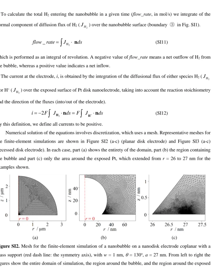
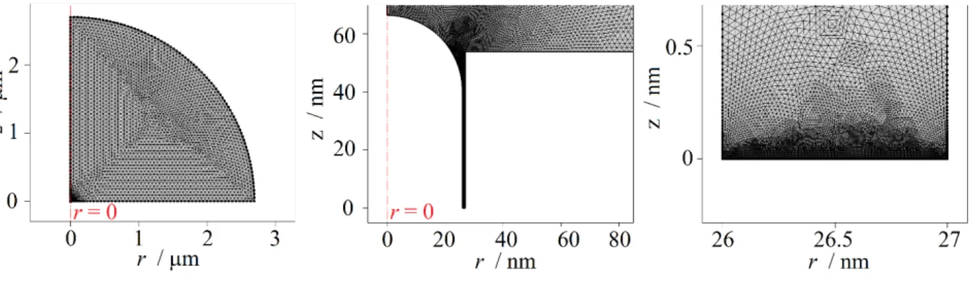
Numerical solution of the equations involves discretization, which uses a mesh. Representative meshes for the finite-element simulations are shown in Figure SI2 (a-c) (planar disk electrode) and Figure SI3 (a-c) (recessed disk electrode). In each case, part (a) shows the entirety of the domain, part (b) the region containing the bubble and part (c) only the area around the exposed Pt, which extended from r = 26 to 27 nm for the examples shown.

(a) (b) (c)

Figure SI2. Mesh for the finite-element simulation of a nanobubble on a nanodisk electrode coplanar with a glass support (red dash line: the symmetry axis), with w = 1 nm, θ = 130o_{, a = 27 nm. From left to right the}

figures show the entire domain of simulation, the region around the bubble, and the region around the exposed Pt.

(a) (b) (c)

Figure SI3. Mesh for the finite-element simulation of a nanobubble at a recessed disk nanoelectrode with w = 1 nm, θ = 130o_{, a = 27 nm, L = 54 nm, H/L = 0.75. From left to right the figures show: the entire domain of}

simulation, the region around the bubble, and the region around the exposed Pt.

While the exact number of mesh elements varied as the width of exposed Pt (w) was varied, in all cases we kept at least 100 elements on boundary ①. When necessary, refinements of the mesh were performed in order to keep both the relative precision of the rate of H2 transport out of the bubble and the electrode current at better

than 1%. The number of mesh elements was increased as the width of exposed Pt (w) was decreased.

Finite element simulations were performed using COMSOL Multiphysics 5.1 (Comsol, Inc.). An automatically generated report detailing all of the meshing parameters and other specifics of the simulations is provided as a separate file Supporting Information 2. Unless stated, the parameters used for the calculations are the following: DH+=9.3x10-9 m2/s, DH2=4.5x10-9 m2/s, T=298.15 K, 𝑐𝑐_Hbulk+ =0.5 mol/L, 𝑐𝑐_Hbulk₂ =0 mol/L, 𝛾𝛾= 0.072 N/m, KH = 0.00078 mol L-1 bar-1.