Yuhong Guo 1 and Dale Schuurmans2 1 Department of Computer and Information Sciences
Temple University Philadelphia, PA 19122, USA
2 Department of Computing Science University of Alberta Edmonton, AB, T6G 2E8, Canada
Abstract. Although multi-label classification has become an increas-ingly important problem in machine learning, current approaches remain restricted to learning in the original label space (or in a simple linear projection of the original label space). Instead, we propose to use ker-nels on output label vectors to significantly expand the forms of label
dependence that can be captured. The main challenge is to reformulate standard multi-label losses to handle kernels between output vectors. We first demonstrate how a state-of-the-art large margin loss for multi-label classification can be reformulated, exactly, to handle output kernels as well as input kernels. Importantly, the pre-image problem for multi-label classification can be easily solved at test time, while the training pro-cedure can still be simply expressed as a quadratic program in a dual parameter space. We then develop a projected gradient descent training procedure for this new formulation. Our empirical results demonstrate the efficacy of the proposed approach on complex image labeling tasks.
1
Introduction
Multi-label classification is a central problem in modern data analysis, where complex data items, such as documents, images and videos, exhibit multiple concepts of interest and thus belong to multiple non-overlapping categories. For example, in text categorization, a news article or web page is often relevant to a set of topics; similarly, in image labeling, an image can contain multiple objects and therefore be assigned multiple class labels. Although multi-label classifi-cation has been well investigated, it continues to receive significant attention. Initial work considered transforming multi-label classification to a set of indepen-dent binary classification problems [1], but this approach proved unsatisfactory as it failed to exploit label interdependence [2]. A key issue has since become capturing label dependence to improve multi-label classification accuracy. Many approaches have been developed to exploit label dependence in multi-label learn-ing, including pairwise dependence methods [3, 4], large-margin methods [5–8],
ranking based methods [9–12], and probabilistic graphical models [13–15]. Un-fortunately, these methods work in the original label space, limiting their ability to capture complex dependence structure in a computationally efficient manner. There has been recent interest in multi-label methods that work in
trans-formed label spaces [16–21], primarily based on low-dimensional projections of
high dimensional label vectors. For example, random projections [16], maximum eigenvalue projections [18, 17], and Gaussian random projections [21] provide techniques for mapping high dimensional label vectors to low dimensional code-words to improve the efficiency of multi-label learning. Canonical correlation analysis (CCA) has also been considered for relating inputs to label projections [20]. However, these projection approaches divide the learning problem into sep-arate dimensionality reduction and training steps, which does not ensure that the reduced output representation is amenable to predictor training. Max margin output coding [19], on the other hand, combines output projection and predic-tion model learning in a joint optimizapredic-tion, but it must consider every label combination while ignoring the residual error from the projected representation back to the original label set. These methods primarily focus on reducing output dimension to improve efficiency, rather than attempt to explicitly capture richer label dependence. Moreover, the proposed label vector projections are limited to linear transformations, which cannot capture nonlinear label dependence.
Instead, in this paper we propose a new multi-label classification approach that uses output kernels to capture more complex nonlinear dependences be-tween labels in a flexible yet tractable manner. Such an approach significantly expands the form of label dependences that can be captured, both at training and test time. Although kernel methods have been widely used for expanding input representations, kernels have yet to be used to explicitly capture nonlin-ear output structure in multi-label classification. We base our formulation on a recent large margin multi-label approach that minimizescalibrated separation
ranking loss [8]. Such a loss achieves state-of-the-art results in multi-label
clas-sification, but it makes kernelization a challenge because it is different from any loss formulation that has been previously shown to be kernelizable. Demonstrat-ing that a tailored multi-label loss can be equivalently re-expressed in terms of output kernels is one of the key contributions of this paper.
After reviewing related work on learning with output kernels in Section 2, we introduce the main multi-label classification formulation we use in Section 3. Our formulation is based on the calibrated separation ranking loss of [8], which we show can be equivalently re-expressed by an output kernel in Section 4. In particular, we produce a quadratic program in dual parameter space that encodes both the outputs and inputs in kernel forms. We also show that the pre-image problem for multi-label classification can be easily solved at test time. A scalable projected gradient descent optimization algorithm is then presented in Section 5. Finally, we conduct experiments on multi-label data in Section 6, and compare to standard multi-label classification. Our results demonstrate the efficacy of the proposed approach when the labels demonstrate complex dependence structure. We conclude the paper with a brief discussion of future work in Section 7.
2
Related Work: Learning with Output Kernels
Although other losses have been re-expressed in terms of output kernels, cur-rent formulations have either assumed a least squares loss or a simple 0-1 mis-classification loss. These standard losses make the extension to output kernels straightforward, but developing a similar extension for the more complex loss we consider for multi-label classification is a greater challenge.
To re-express a problem in terms of a kernel over an output space Y, one assumes there is a feature mapϕ:Y → HY that maps each output label vector
y into a new representation ϕ(y). A kernel between output vectors can then be defined by an inner product between two output label vectors in the new representation space (formally, in a reproducing kernel Hilbert space [22, 23]). Such formulations have already been explored in machine learning, but they are often hampered by an intractable pre-image problem at test time [24]: for a given test instance, even though the similarity between any candidate output and training outputs can be determined easily, the search for the optimal test output can be a hard computational problem [23]. We will seek to avoid such intractability in our method.
Previous work on multi-class (not multi-label) classification learning has demonstrated that training can be equivalently expressed in terms of an out-put kernel when the classes are disjoint [25–27]. In particular, extensions to output kernels have been achieved for unsupervised and semi-supervised logistic regression training with hidden output variables [25], and convex reformulations of unsupervised and semi-supervised training of support vector machines [26, 27]. It turns out that output kernelization is trivially achieved in this special case simply by using the linear kernel between class indicator vectors. However, in these contexts, this extension is only used to achieve convex reformulations of the training process, not to expand the set of output dependence structures that can be captured. Moreover, these approaches generally involve learning an output kernel via expensive semi-definite programming.
Applying kernel methods in the output space has also been exploited in regression methods for structured output learning [28–37]. For example, in [28– 30], regression models are trained by least squares to predict an output kernel matrix Ky from an input kernel matrix Kx. In [35, 36], similar methods are developed for transductive link prediction and regression to fixed output kernel values extracted from given link labels. The methods in [32–34] extend tree-based regression to kernelized output spaces for structured data, but do not exploit kernels defined over the input space. A related approach is to adopt a joint kernel over input/output pairs [38]. Unfortunately, all of these regression based approaches require the solution of a difficult pre-image problem to recover the predictions for any test instance. Furthermore, none of these methods directly address multi-label classification.
Other recent work has proposed to learn a covariance matrix between labels in a multi-label setting to capture dependence [8, 39–41]. However, these methods do not produce a kernel representation in the output space; rather, their output representations remain restricted to the original label set. Our goal in this paper
is to exploit kernels to capture complex nonlinear dependence between labels for multi-label classification.
3
Background: Large Margin Multi-label Classification
To address multi-label classification we consider a large margin approach to clas-sifier training. By optimizing a discriminative objective, large margin methods have proved successful in practice, achieving both good generalization perfor-mance and computational efficiency. We will therefore focus on the calibrated separation ranking loss criterion of [8], which achieves state-of-the-art multi-label classification results while retaining the simplicity and efficiency of a large margin approach. This loss expresses the sum of two large margin losses, one between the prediction value of the least positive label response and the value of a dummy threshold class, and the other between the prediction value of the least negative label response and the value of the dummy threshold class. Such an approach allows the predictions to be coordinated across different labels sim-ply by using a shared adaptive threshold, rather than suffering the intractability of considering all label subsets [42] or even the cost of considering all label pairs (followed by a difficult labeling problem at test time) [9].
Definitions and Notation:To formulate the approach, we introduce some definitions and notation. X andY denote the input and output spaces respec-tively. Below we will use capital letters to denote matrices, bold lower-case letters to denote column vectors, and regular lower-case letters to denote scalars, unless special declaration is given. Given a vectorx,kxk2denotes its Euclidean norm.
Given a matrixX,kXk2
F denotes its Frobenius norm. We use Xi: to denote the
ith row of a matrix X, use X:j to denote thejth column of X, and useXij to denote the entry at theith row andjth column ofX. For matrices, we usekXk
to refer to a generic norm onX, and usetrto denote trace. We useIdto denote a d×didentity matrix; and use1to denote a column vector with all 1 entries, generally assuming its length can be inferred from context. Inequalities≥,≤are applied entrywise. For a boolean label matrixY we let ¯Y denote its complement
¯
Y =11⊤−Y. Finally, we use◦to denote Hadamard (componentwise) product. To introduce the underlying approach, assume one is given an input data matrixX ∈Rt×dand label indicator matrixY ∈ {0,1}t×L, whereLdenotes the number of classes. For convenience, we assume a feature functionφ:X → HX
is provided that maps each input vector x into a new representation φ(x) in the Hilbert space HX. Therefore the input dataX can be putatively converted (row-wise) into a feature matrix Φ :=φ(X). Given an input instance x, an L dimensional response vectors(x) :=φ(x)⊤W can be recovered using parameter
matrixW, giving a “score” for each label. These scores can then be compared to a threshold values0(x) :=φ(x)⊤u, using a parameter vectoru, to determine
which labels are to be ‘on’ and ‘off’ respectively. In particular, the classification of a test examplexis determined by
yl∗= arg max
for each candidate labell∈ {1, ..., L}.
To learn the parameters,W andu, of this score based multi-label classifier, we consider the calibrated separation ranking loss of [8], given by:
max l∈Yi:
(1 +s0(Xi:)−sl(Xi:))++ max ¯
l∈Yi¯:
(1 +s¯l(Xi:)−s0(Xi:))+. (2)
Intuitively, this training loss encourages the model to produce scores a minimum margin above the threshold value for ‘on’ labels, and a minimum margin below the threshold value for ‘off’ labels. In previous work, [8] demonstrates that this loss achieves state-of-the-art generalization performance across a range of multi-label data sets while retaining efficient training and test procedures.
To allow efficient optimization, training with the calibrated separation rank-ing loss under standard Euclidean regularization of the parameters can be formu-lated as a convex quadratic program (where we have rewritten the formulation given in [8] in a more compact matrix form):
min W,u,ξ,η α 2(kWk 2 F +kuk22) +1⊤ξ+1⊤η (3) s.t. ξ≥0, ξ1⊤ ≥Y ◦(11⊤+Φ(u1⊤−W)), η≥0, η1⊤ ≥Y¯ ◦(11⊤−Φ(u1⊤−W)).
Training with respect to a kernel over the input space can then be easily achieved by considering the dual of this quadratic program [8], given by:
max M,N 1 ⊤(M +N)1− 1 2αtr((M−N) ⊤K(M −N)(I+11⊤)) (4) s.t. M ≥0, M1≤1, M ◦Y¯ = 0, N ≥0, N1≤1, N◦Y = 0,
where K =ΦΦ⊤,M and N are botht×L dual parameter matrices. Here the primal solution is related to the dual solution by:
W = α1X⊤(M−N), u= 1
αX
⊤(N−M)1. (5)
Thus, one reaches the conclusion that the original training problem can be ex-pressed in terms of a kernel on the input space. However, the target output labels appear linearly in the constraints in both the primal and dual formulations. It is not obvious how these constraints can be equivalently re-expressed in terms of a kernel between output vectors.
4
Multi-label Classification with Output Kernels
A main contribution of this paper is to derive an equivalent formulation to (4) that is expressed entirely in terms of a kernel between output vectors. Such a formulation allows one to express multi-label classification in a manner that can flexibly capture nonlinear dependence between output labels.
We start by making the assumption thatL < t; that is, there are more train-ing examples than labels, which is a natural assumption in many applications. First observe that, sinceM ≥0 and ¯Y ≥0 in (4), the constraintM◦Y¯ = 0 can be equivalently re-expressed as tr(M⊤Y¯) = 0; similarly, the constraintN ◦Y = 0
can be equivalently re-expressed as tr(N⊤Y) = 0. This allows the quadratic
program (4) to be simplified somewhat to: max M,N 1 ⊤(M +N)1− 1 2αtr((M −N) ⊤K(M−N)(I+11⊤) (6) s.t. M ≥0, M1≤1, tr(M⊤Y¯) = 0, N≥0, N1≤1, tr(N⊤Y) = 0.
Unfortunately it is still not obvious that (6) can be converted to a form that involves only inner products between label vectors. However, we will see now that this can be achieved in two steps.
The first key step is to consider an expanded set of inner products; that is, consider the set of inner products not just between label vectors in Y but also between complements of these label vectors (i.e. in ¯Y) and the canonical set of single class indicator vectors (i.e. in IL). In particular, consider the expanded (L+ 2t)×Llabel matrixS= [I;Y; ¯Y] (i.e., stacked vertically) from which one can form the augmented inner product matrix
Q=SS⊤ = I Y⊤ Y¯⊤ Y Y Y⊤ YY¯⊤ ¯ Y Y Y¯ ⊤ Y¯Y¯⊤ . (7)
This augmented kernel matrix embodies useful information for reformulating the training problem (6). For example, one important property it satisfies is:
Q1= 1+ (Y + ¯Y)⊤1 Y1+Y(Y + ¯Y)⊤1 ¯ Y1+ ¯Y(Y + ¯Y)⊤1 = 1+11⊤1 Y1+Y11⊤1 ¯ Y1+ ¯Y11⊤1 = (t+1) 1 Y1 ¯ Y1 = (t+1)S1,(8)
which will be helpful below.
The second key step is to apply a change of variables by the following lemma.
Lemma 1. For anyS defined as above, and for any M ≥0 andN ≥0, there
must exist two real value matricesΩ≥0andΓ ≥0of sizet×(L+ 2t)such that
M =ΩS andN=Γ S. (9)
Proof. First observe thatM =ΩS defines a system of tlinear equations where
the ith equation is given by Mi: = Ωi:S. By Farkas’ Lemma, givenMi: ∈ RL
andS∈R(L+2t)×L, exactly one of the following two statements must be true: 1. There exists anω∈R(L+2t)such thatMi:=ω⊤S andω≥0.
2. There exists az∈RL such thatSz≥0 andMi:z<0.
Assume that there exists a z∈RL such that Mi:z<0. Then, sinceMi: ≥0,z
has an identity submatrix, we conclude that thejth entry ofSzmust be negative. Therefore the second statement of Farkas’ lemma cannot hold. According to the first statement, we therefore know that for the given S and Mi: ≥ 0, there
must exist an ω ≥0 such that Mi: =ω⊤S. Finally, by taking all of the linear
systems into consideration, we conclude that for anyM ≥0 there must exist an Ω∈Rt×(L+2t), Ω≥0 that satisfies (9). An identical argument can be used to establish the condition between the N≥0 andΓ ≥0 matrices.
Next, by introducing the expanded label kernel matrixQand by making the variable substitution suggested by Lemma 1, the main result can be established: the original training problem (6) can be re-expressed in terms of inner products between output vectors from the augmented set of label vectorsS.
Proposition 1. By applying the variable substitution justified by Lemma 1 and using (7) and (8), the quadratic program (6) can be equivalently re-expressed as:
max Ω,Γ 1 ⊤(Ω+Γ)Q1− 1 2αtr((Ω−Γ) ⊤K(Ω−Γ)((t+1)Q+ 1 t+1Q1(Q1) ⊤)) (10) s.t. Ω≥0, ΩQ1≤(t+ 1)1, tr(ΩQB) = 0, Γ ≥0, Γ Q1≤(t+ 1)1, tr(Γ QA) = 0;
where A= [OL,t;It;Ot],B= [OL,t;Ot;It],Itis a t×t identity matrix, Ot is a
t×t matrix with all 0 values, andOL,t is aL×t matrix with all 0 values.
Proof. Using the substitution (9), the objective in (6) can be rewritten as:
(6) =1⊤(Ω+Γ)S1− 1
2αtr((Ω−Γ)
⊤K(Ω−Γ)(SS⊤+S1(S1)⊤)). (11)
Next, observe that usingQ=SS⊤ andS1= 1
t+1Q1, the objective (11) can be
further rewritten as:
(11) = t+11 1⊤(Ω+Γ)Q1−21αtr((Ω−Γ)⊤K(Ω−Γ)(Q+(t+1)1 2Q1(Q1)
⊤)),(12)
which, multiplying by t+ 1, leads to the form stated in the proposition. Finally, we consider the constraints in (6). For the equality constraints, using the non-negativity of the matrices involved and applying the previous substitu-tions one obtains:
tr(M⊤Y¯) =tr(ΩSY¯⊤) =tr(Ω[ ¯Y⊤;YY¯⊤; ¯YY¯⊤]) =tr(ΩQB) = 0, (13) tr(N⊤Y) =tr(Γ SY⊤) =tr(Γ[Y⊤;Y Y⊤; ¯Y Y⊤]) =tr(Γ QA) = 0. (14)
For the middle inequality constraints, applying the same substitution (9) yields: M1=ΩS1= 1
t+1ΩQ1≤1, (15)
N1 =Γ S1= 1
t+1Γ Q1≤1. (16)
Finally, for the non-negativity constraints M ≥0 andN ≥0, Lemma 1 shows that these can be equivalently enforced by assertingΩ≥0 andΓ ≥0.
4.1 Extension to Output Kernels for Multi-label Classification
Since Proposition 1 shows that minimizing the regularized calibrated separation ranking loss can be expressed in terms of inner products between label vectors, an extension to output kernels can be achieved in the obvious way. As before, one assumes a feature map ϕ : Y → HY that transforms each label vector y
into a new representationϕ(y) in the Hilbert spaceHY, hence a kernel between output vectors can be defined by an inner product between two output label vectors in the new representation space (an RKHS). In practice, one chooses a positive semidefinite kernel function κy(·,·) such that conceptually κy(y,y˜) = ϕ(y)⊤ϕ(˜y) (where we are assuming this denotes inner product in the implied
reproducing kernel Hilbert space). In this way, the matrixQcan be constructed asQ=κy(S, S), where conceptuallyκy(S, S) =ϕ(S)ϕ(S)⊤.
However, there is an important catch: in this case it turns out that, unlike in-put kernelization (or outin-put kernelization for least squares regression), not every valid kernel is suitable as an output representation for multi-label classification. Specifically, the optimization formulation above is only well posed for a subset of possible output kernel functions (although any input kernel can still be used). To preserve equivalence between the output kernelized form (10) and the dual form (4) established in Proposition 1, we at least require that the kernel matrix Q be doubly non-negative; i.e., Q 0, andQ ≥0 entrywise. Furthermore, to preserve Lemma 1,Qmust also preserve orthogonality; that is, ifYi:Yj⊤: = 0 then
Qij = 0. Therefore, overall, for any output kernel function κy that one would wish to use for multi-label classification training the following set of constraints must be satisfied: positive semi-definiteness, κy(S, S)0 for any finiteS; non-negativity, κy(y,y˜)≥0 for ally ∈ {0,1}L and ˜y∈ {0,1}L; and orthogonality,
y⊤˜y= 0 must implyκy(y,y˜) = 0.
These properties are obviously satisfied by the linear kernel used to derive Proposition 1. However, in addition to the linear kernel, other kernels common in document and language modeling are appropriate for this setting [43]. One particularly useful family of kernels that satisfy these properties are the homo-geneous polynomial kernels:
Kpoly(y,y˜) = k
X
i=1
wi(y⊤˜y)i, (17) wherew≥0 is a vector of non-negative weights. Unfortunately, many standard kernels, such as the Gaussian (RBF) kernel are not suitable, since by violating the constraints it blocks all nonzero solutions to (10). Below we find that the simple weighted polynomial kernels allow sufficient flexibility in capturing nonlinear dependence to achieve positive results in some real world multi-label data sets.
4.2 Classification of Test Instances
Although Proposition 1 shows that training for multi-label classification can be formulated in terms of a kernel between label vectors, this does not imply
that classifying new instances x at test time will be necessarily easy. In fact, for regression formulations, test prediction generally involves solving a hard pre-image problem [23, 24]. Fortunately, the pre-pre-image problem can be efficiently solved for multi-label classification, even when there are an exponential (2L) number of label vectors to consider.
After solving the training problem (10) one obtains the global solution (Ω, Γ), which can be used to efficiently classify a new test instance as follows. Let κx and κy denote the input and output kernels respectively. Conceptually, we can think of these as evaluating an inner product between feature representations of the inputs and outputs as κx(x,x˜) =φ(x)⊤φ(˜x) and κy(y,y˜) =ϕ(y)⊤ϕ(˜y)
respectively. Then from the optimal parameters, we can conceptually recover the solution (M, N) to the original dual problem (4) via
M =Ωϕ(S) andN =Γϕ(S). (18)
Using (1), the optimal parameters (W,u) for the original problem (3) are: W =α1φ(X)⊤(Ω−Γ)ϕ(S), (19) u= 1 αφ(X) ⊤(Γ−Ω)ϕ(S)1= 1 α(t+1)φ(X) ⊤(Γ−Ω)Q1. (20)
Finally, recall the classification rule used for multi-label assignment (1). Given a new test instancex∈Rd, we will determine its labels by computing the score function values s(x) = [s1(x),· · ·,sL(x)] and s0(x); that is, the label vector y
for x is then given by aL×1 indicator vector where yl = 1 if sl(x)≥ s0(x),
yl = 0 otherwise. Fortunately, these score values can be efficiently computed directly from the recovered (Ω, Γ) parameters via:
s0(x) =φ(x)u= α(t1+1)κx(x, X)(Γ −Ω)Q1, (21)
sl(x) =φ(x)Wϕ(1l) = 1
ακx(x, X)(Ω−Γ)κy(S,1l), ∀l= 1,· · ·, L; (22) where 1l denotes a vector with 1 as its lth entry and 0 elsewhere. Thus, the multi-label assignment to test instancexcan be efficiently computed.
5
A Scalable Training Method
One of the main challenges with this formulation is that the quadratic program-ming problem (10) is defined over (L+ 2t)×tmatrix variables, which makes the training problem challenging for standard solvers. Instead, we develop a row-wise projected gradient method to achieve a more scalable approach.
First note that the optimization problem (10) can be written in a more compact form. Replace Ω and Γ with Λ= [Ω, Γ]. LetC = [IL+2t;OL+2t] and
D = [OL+2t;IL+2t], such that Ω = ΛC and Γ = ΛD. Furthermore, let P = 1 α(C−D)((t+1)Q+ 1 t+1Q1(Q1) ⊤))(C−D)⊤;E = ((C+D)Q11⊤)⊤;a= 1 t+1CQ1;
more succinctly as: min Λ 1 2tr(Λ ⊤KΛP)−tr(ΛE⊤) (23) s.t. Λ≥0, Λa≤1, tr(ΛG⊤) = 0, Λb≤1, tr(−ΛF⊤) = 0.
The key property of this quadratic program is that the constraints decom-pose row-wise. This allows us to use a row-wise coordinate descent procedure to achieve scalability. Consider theith row ofΛ, assuming all other rows are fixed. An update to rowΛi:can be expressed asΛ=Λ+1i(z⊤−Λi:), where1iis a col-umn vector of zeros with a single 1 in theith position. LetΛ¯i: :=Λ−1iΛi:. The
objective function f(Λ) := 1 2tr(Λ
⊤KΛP)−tr(ΛE⊤) of the quadratic program
can be re-expressed as a functiongover the single row update zsuch that: g(z) =f(Λ+1i(z⊤−Λi:)) =f(Λ¯i:+1iz⊤) = 1 2Kii(z ⊤ Pz) + (Ki:Λ¯i:P−Ei:)z+const = 12Kii(z⊤Pz) + (Ki:ΛP−KiiΛi:P−Ei:)z+const (24)
which yields the row optimization problem: min
z
g(z) s.t. z≥0, z⊤a≤1, Gi:z= 0, z⊤b≤1, Fi:z= 0. (25)
The update of the ith row only affects other rows through the Ki:ΛP term.
Therefore, we maintain a matrix U = KΛP that can be updated locally after an update toΛi:, byU =U+K:i(z⊤−Λi:)P. To ensure that progress is always
made, while maintaining scalability, we use a row-wise steepest descent method. For the objective functiong(z), its gradient vector is given by:
g=dg(z)
dz =KiiPz+ (Ki:ΛP−KiiΛi:P−Ei:) ⊤
, (26) which can be efficiently computed. Since the constraints on z are simple, this gradient vector can be efficiently projected to a feasible directiond. Because the objective f has a simple quadratic form, the optimal step size in the feasible directiondcan be computed in closed form. Thus, optimal updates can be made by locally operating on each row ofΛin succession. We have found this approach to be reasonably effective in our experiments below.
6
Experiments
To evaluate the proposed approach, we conducted experiments on a multi-label classification image set, scene, and a set of multi-label classification tasks con-structed from a real-world image data set,MIRFlickr. We compared the proposed output kernel approach to a number of large margin multi-label classification methods, and to an output-kernel based least square regression method.
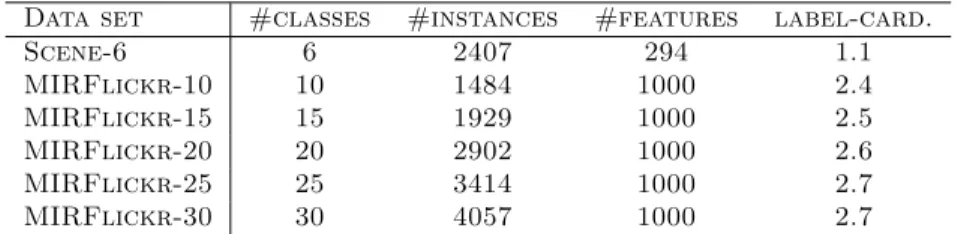
Table 1.Properties of the multi-label data sets used in the experiments.
Data set #classes #instances #features label-card.
Scene-6 6 2407 294 1.1 MIRFlickr-10 10 1484 1000 2.4 MIRFlickr-15 15 1929 1000 2.5 MIRFlickr-20 20 2902 1000 2.6 MIRFlickr-25 25 3414 1000 2.7 MIRFlickr-30 30 4057 1000 2.7 6.1 Experimental Setting
Data Sets We focused on image data sets for these experiments, since image data usually exhibits highly nonlinear semantic dependence between labels. The
scene[44] data set has 2407 images and only 6 classes, whereas theMIRFlickr[45]
data set contains 25,000 images and 457 classes. Although MIRFlickr has a very large number of classes, the labels appear in a very sparse manner. One key prop-erty of multi-label data sets is their label cardinality [42]; the average number of labels assigned to each instance. If the label cardinality of a data set is close to 1, the task reduces to a standard single label classification task, and there will not be any significant label dependence to capture. The effectiveness of multi-label learning can therefore primarily be demonstrated on data sets whose label cardi-nality is reasonably large and complex. We thus constructed a set of multi-label classification tasks from the MIRFlickr image data set that maintained reason-able label cardinalities while ranging across a set of different numbers of classes. Specifically, we constructed five multi-label subsets, 10,
MIRFlickr-15, MIRFlickr-20, MIRFlickr-25, and MIRFlickr-30, by randomly selecting L
classes, for L ∈ {10,15,20,25,30} respectively, to achieve a reasonable level of label cardinality in each case; see Table 1 for a summary.
Approaches Our proposed approach (LM-K) is based on using output kernels to capture nonlinear label dependence during training. In these experiments, we employed the homogeneous polynomial kernels as defined in (17). Withk ≥2, these polynomial kernels can automatically encode pairwise and higher-order label dependence structures in an expanded output space.
We compare the proposed approach to a number of state-of-the-art multi-label classification methods to investigate the consequences of using nonlinear output kernels. These competitors were: (1) the large margin method based on the calibrated separation ranking loss (CSRL) [8]; (2) the pairwise rank-ing loss SVM (Rank) proposed in [9], which first trains a large margin ranking model and then learns the threshold of the multi-label predications using a least-square method; and (3) the max-margin multi-label classification method (M3L) proposed in [7], which takes prior knowledge about the label correlations into account. None of these methods use output kernels. Therefore, we also compare the proposed method with a least squares regression method that uses output kernels (LS-K), thresholding its predictions for multi-label classification.
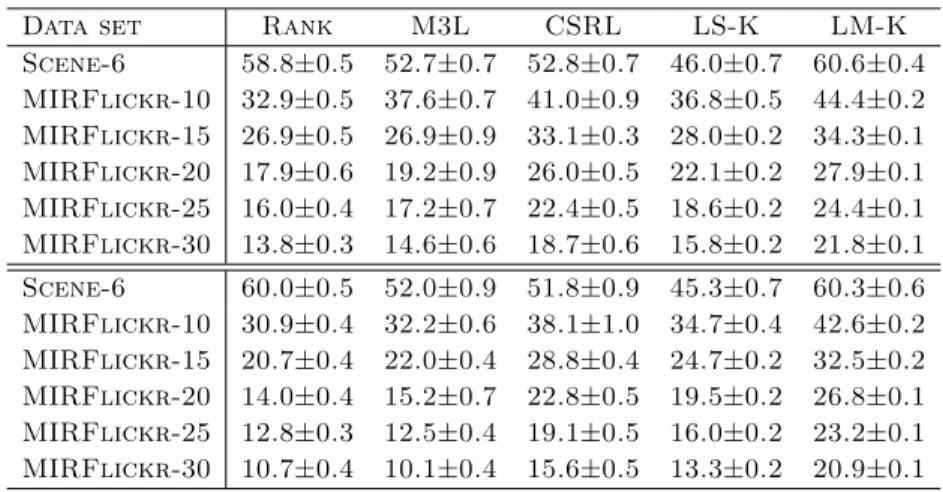
Table 2. Summary of the performance (%) for the compared methods in terms of micro-F1 (top section) and macro-F1 (bottom section).
Data set Rank M3L CSRL LS-K LM-K Scene-6 58.8±0.5 52.7±0.7 52.8±0.7 46.0±0.7 60.6±0.4 MIRFlickr-10 32.9±0.5 37.6±0.7 41.0±0.9 36.8±0.5 44.4±0.2 MIRFlickr-15 26.9±0.5 26.9±0.9 33.1±0.3 28.0±0.2 34.3±0.1 MIRFlickr-20 17.9±0.6 19.2±0.9 26.0±0.5 22.1±0.2 27.9±0.1 MIRFlickr-25 16.0±0.4 17.2±0.7 22.4±0.5 18.6±0.2 24.4±0.1 MIRFlickr-30 13.8±0.3 14.6±0.6 18.7±0.6 15.8±0.2 21.8±0.1 Scene-6 60.0±0.5 52.0±0.9 51.8±0.9 45.3±0.7 60.3±0.6 MIRFlickr-10 30.9±0.4 32.2±0.6 38.1±1.0 34.7±0.4 42.6±0.2 MIRFlickr-15 20.7±0.4 22.0±0.4 28.8±0.4 24.7±0.2 32.5±0.2 MIRFlickr-20 14.0±0.4 15.2±0.7 22.8±0.5 19.5±0.2 26.8±0.1 MIRFlickr-25 12.8±0.3 12.5±0.4 19.1±0.5 16.0±0.2 23.2±0.1 MIRFlickr-30 10.7±0.4 10.1±0.4 15.6±0.5 13.3±0.2 20.9±0.1 6.2 Experimental Results
Classification Results We first conducted a set of experiments on the six multi-label data sets by randomly sampling 300 labeled images as training data and holding out the remaining as test data. The intent is to investigate how well each approach can exploit label dependence when there are limited training instances available. In the experiments, we set the trade-off parameter α= 0.1 for the proposed approach andCSRL, and set the trade-off parameters forRank
and M3Lcorrespondingly withC = 10. We used the linear input kernel for all methods. ForLS-K andLM-K, we used the polynomial output kernel given in (17) with maximum degree k= 2, with weightsw1=w2 = 1. This polynomial
kernel automatically encodes all pairwise label dependency structures within the induced high dimensional output space. We repeated each experiment 10 times and report the average multi-label classification performance in terms of micro-F1 and macro-F1 in Table 2.
From Table 2, one can observe that the difficulty of the learning problem increases with label set size, causing degradation in the performance of all meth-ods. However, with a nonlinear output kernel, the proposed approach LM-K
consistently outperforms the three state-of-the-art large margin multi-label clas-sification methods, Rank, M3L and CSRL, across all the data sets with differ-ent numbers of classes. It also significantly outperforms least-squares regression method with the same output kernel,LS-K. These results suggest that a nonlin-ear output kernel is indeed useful for improving multi-label classification models in a setting with interesting label dependencies. Here the proposed approach ap-pears to provide an effective method for exploiting nonlinear dependence struc-ture through the use of a polynomial output kernel.
Polynomial Kernels Based on the definition of homogeneous polynomial ker-nels given in (17), one can produce many different kerker-nels with different weights
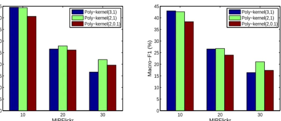
10 20 30 0 5 10 15 20 25 30 35 40 45 MIRFlickr Micro−F1 (%) Poly−kernel(3,1) Poly−kernel(2,1) Poly−kernel(2,0.1) 10 20 30 0 5 10 15 20 25 30 35 40 45 MIRFlickr Macro−F1 (%) Poly−kernel(3,1) Poly−kernel(2,1) Poly−kernel(2,0.1)
Fig. 1.Comparison of different polynomial output kernels on the MIRFlickr data sets.
{wi} and different maximum degree k. We next investigated the influence of alternative output kernels on multi-label classification. We considered three dif-ferent polynomial kernels by varying the degree number and the weights: (1) Poly-kernel(3,1) uses degree up to k = 3 and weights w1 = w2 = w3 = 1;
(2) Poly-kernel(2,1) uses degree up to k = 2 and weights w1 = w2 = 1; and
(3) Poly-kernel(2,0.1) uses degree up to k = 2 but with weights w1 = 1 and
w2= 0.1. Evidently the first polynomial kernel with maximum degree 3
consid-ers triplet-wise label dependencies, whereas the other two kernels only consider pairwise label dependence. Moreover, the last kernel put relatively less weight on the higher order dependence features.
We conducted experiments on three MIRFlickr data sets, MIRFlickr-10,
MIRFlickr-20, and MIRFlickr-30, using the same setting as above. The results
are reported in Figure 1, in terms of micro-F1 measure and macro-F1 measure. From these results one can see that even though it embodies more complex la-bel features, Poly-kernel(3,1) demonstrates inferior performance when the class number increases, compared to the less complex Poly-kernel(2,1). This suggests that Poly-kernel(3,1) can over-fit when the classification problem gets more com-plex given limited training data. On the other hand, Poly-kernel(2,0.1) further suppresses the influence of the higher order label features, and demonstrates inferior performance compared to Poly-kernel(3,1) when there are fewer labels. The intermediate Poly-kernel(2,1) demonstrates good performance on all three data sets. These results suggest selecting output kernels with the right complex-ity is important, and pairwise label features are very useful for encoding label dependence structure, somewhat vindicating an original intuition about multi-label classification [9]. A proper output kernel should give proper consideration over the pairwise feature expansions, and the complexity of the problem.
Performance vs Training Size With a modest training size, we have demon-strated that the proposed approach can effectively improve multi-label classifica-tion performance by exploiting the label dependence informaclassifica-tion and structure
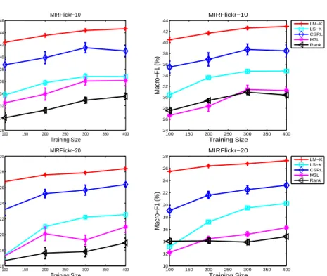
100 150 200 250 300 350 400 28 30 32 34 36 38 40 42 44 46 MIRFlickr−10 Training Size Micro−F1 (%) 100 150 200 250 300 350 400 24 26 28 30 32 34 36 38 40 42 44 MIRFlickr−10 Training Size Macro−F1 (%) LM−K LS−K CSRL M3L Rank 100 150 200 250 300 350 400 16 18 20 22 24 26 28 30 MIRFlickr−20 Training Size Micro−F1 (%) 100 150 200 250 300 350 400 10 12 14 16 18 20 22 24 26 28 MIRFlickr−20 Training Size Macro−F1 (%) LM−K LS−K CSRL M3L Rank
Fig. 2.Performance vs training size.
through the nonlinear output kernel. There remains a question of how the behav-ior of the various methods would change with increasing sample size. To answer this question, we conducted experiments with a number of different training sizes, t∈[100,200,300,400] on two of the data sets,MIRFlickr-10andMIRFlickr-20. We otherwise used the same experimental setting as above. The average re-sults and standard deviations in terms of micro-F1 and macro-F1 measure on these two data sets are plotted in Figure 2. Here, one can see that with increas-ing trainincreas-ing size, the performance of all methods generally improves. However, the proposed approach with polynomial output kernel consistently outperforms the other methods across all training sizes, evaluation measures, and data sets. These results again demonstrate the efficacy of the proposed approach for using nonlinear output kernel to capture label dependency of multi-label learning.
7
Conclusion
We have introduced a new form of multi-label classification learning that uses an output kernel between multi-label output vectors to capture a rich set of non-linear dependences between output labels, while retaining a tractable equivalent formulation as a quadratic program. Although the resulting quadratic programs
are expanded, a scalable training algorithm can be based on example-wise pro-jected gradient descent. The resulting method demonstrates advantages in multi-label image classification experiments over standard linear-output approaches.
In addition to investigating the benefits of alternative output kernels and alternative scaling strategies, an important direction for future research is to investigate other important loss formulations in machine learning, to determine whether they too might be amenable to an equivalent kernelized approach.
References
1. Joachims, T.: Text categorization with support vector machines: learn with many relevant features. In: Proc. of ECML. (1998)
2. McCallum, A.: Multi-label text classification with a mixture model trained by EM. In: AAAI Workshop on Text Learning. (1999)
3. Zhu, S., Ji, X., Xu, W., Gong., Y.: Multi-labelled classification using maximum entropy method. In: SIGIR-05. (2005)
4. Petterson, J., Caetano, T.: Submodular multi-label learning. In: Advances in Neural Information Processing Systems (NIPS). (2011)
5. Kazawa, H., Izumitani, T., Taira, H., Maeda, E.: Maximal margin labeling for multi-topic text categorization. In: NIPS 17. (2004)
6. Godbole, S., Sarawagi, S.: Discriminative methods for multi-labeled classification. In: PAKDD. (2004) 22–30
7. Hariharan, B., Vishwanathan, S., Varma, M.: Efficient max-margin multi-label classification with applications to zero-shot learning. Machine Learning88(2012) 8. Guo, Y., Schuurmans, D.: Adaptive large margin training for multilabel
classifica-tion. In: Proc. of AAAI. (2011)
9. Elisseeff, A., Weston, J.: A kernel method for multi-labelled classification. In: NIPS. (2001)
10. Schapire, R., Singer, Y.: Boostexter: A boosting-based system for text categoriza-tion. Machine Learning Journal (2000) 135–168
11. Shalev-Shwartz, S., Singer, Y.: Efficient learning of label ranking by soft projections onto polyhedra. JMLR7(2006) 1567–1599
12. Fuernkranz, J., Huellermeier, E., Mencia, E., Brinker, K.: Multilabel classification via calibrated label ranking. Machine Learning73(2) (2008)
13. Ghamrawi, N., McCallum, A.: Collective multi-label classification. In: Proc. of CIKM. (2005)
14. Zaragoza, J., Sucar, L., Morales, E., Bielza, C., Larranaga, P.: Bayesian chain classifiers for multidimensional classification. In: Proc. of IJCAI. (2011)
15. Guo, Y., Gu, S.: Multi-label classification using conditional dependency networks. In: Proc. of IJCAI. (2011)
16. Hsu, D., Kakade, S., Langford, J., Zhang, T.: Multi-label prediction via compressed sensing. In: Proceedings NIPS. (2009)
17. Chen, Y., Lin, H.: Feature-aware label space dimension reduction for multi-label classification. In: Proceedings NIPS. (2012)
18. Tai, F., Lin, H.: Multi-label classification with principal label space transformation. In: Proc. 2nd International Workshop on learning from Multi-Label Data. (2010) 19. Zhang, Y., Schneider, J.: Max margin output coding. In: Proc. ICML. (2012) 20. Zhang, Y., Schneider, J.: Multi-label output codes using canonical correlation
21. Zhou, T., Tao, D., Wu, X.: Compressed labeling on distilled labelsets for multi-label learning. Machine Learning88(2012) 69–126
22. Kimeldorf, G., Wahba, G.: Some results on tchebycheffian spline functions. Journal of Mathematical Analysis and Applications33(1971) 82–95
23. Schoelkopf, B., Smola, A.: Learning with Kernels: Support Vector Machines, Reg-ularization, Optimization, and Beyond. MIT Press (2002)
24. Huang, D., Tian, Y., De la Torre, F.: Local isomorphism to solve the pre-image problem in kernel methods. In: Proceedings CVPR. (2011)
25. Guo, Y., Schuurmans, D.: Convex relaxations of latent variable training. In: Proceedings of Advances in Neural Information Processing Systems (NIPS). (2007) 26. Xu, L., Schuurmans, D.: Unsupervised and semi-supervised multi-class support
vector machines. In: Proceedings AAAI. (2005)
27. Xu, L., Wilkinson, D., Southey, F., Schuurmans, D.: Discriminative unsupervised learning of structured predictors. In: Proceedings ICML. (2006)
28. Cortes, C., Mohri, M., Weston, J.: A general regression technique for learning transductions. In: Proceedings ICML. (2005)
29. Weston, J., Chapelle, O., Elisseeff, A., Schoelkopf, B., Vapnik, V.: Kernel depen-dency estimation. In: Proceedings NIPS. (2002)
30. Wang, Z., Shawe-Taylor, J.: A kernel regression framework for SMT. Machine Translation24(2) (2010) 87–102
31. Micchelli, C., Pontil, M.: On learning vector-valued functions. Neural computation 17(1)(2005) 177–204
32. Geurts, P., Wehenkel, L., d’Alch´e Buc, F.: Kernelizing the output of tree-based methods. In: Proceedings ICML. (2006)
33. Geurts, P., Wehenkel, L., d’Alch´e Buc, F.: Gradient boosting for kernelized output spaces. In: Proceedings ICML. (2007)
34. Geurts, P., Touleimat, N., Dutreix, M., d’Alch´e Buc, F.: Inferring biological net-works with output kernel trees. BMC Bioinformatics8(S-2) (2007)
35. Brouard, C., d’Alch´e Buc, F., Szafranski, M.: Semi-supervised penalized output kernel regression for link prediction. In: Proceedings ICML. (2011)
36. Brouard, C., Szafranski, M.: Regularized output kernel regression applied to protein-protein interaction network inference. In: NIPS MLCB Workshop. (2010) 37. Kadri, H., Duflos, E., Preux, P., Canu, S., Davy, M.: Nonlinear functional
regres-sion: a functional RKHS approach. In: Proceedings AISTATS. (2010)
38. Weston, J., Schoelkopf, B., Bousquet, O.: Joint kernel maps. In: Proceedings of the International Work-Conference on Artificial Neural Networks(IWANN). (2005) 39. Zhang, Y., Yeung, D.: A convex formulation for learning task relationships in
multi-task learning. In: Proceedings UAI. (2010)
40. Dinuzzo, F., Fukumizu, K.: Learning low-rank output kernels. In: Proceedings ACML. (2011)
41. Dinuzzo, F., Ong, C., Gehler, P., Pillonetto, G.: Learning output kernels with block coordinate descent. In: Proceedings ICML. (2011)
42. Tsoumakas, G., Katakis, I.: Multi-label classification: An overview. International Journal of Data Warehousing and Mining (2007)
43. Shawe-Taylor, J., Cristianini, N.: Kernel Methods for Pattern Analysis. Cambridge University Press (2004)
44. Boutell, M., Luo, J., Shen, X., Brown, C.: Learning multi-label scene classiffication. Pattern Recognition37(9) (2004) 1757–1771
45. Huiskes, M., Lew, M.: The MIR flickr retrieval evaluation. In: Proc. of ACM international conference on Multimedia information retrieval. (2008)