Hierarchical and spline-based models in space-time disease mapping

(1)

Departamento de Estadística e Investigación Operativa

PhD Thesis

Hierarchical and spline-based models

in space-time disease mapping

Author:

Aritz Adin Urtasun

Supervisors:

Dr. María Dolores Ugarte Martínez

Dr. Tomás Goicoa Mangado

(2)

(3)

Dr. MARÍA DOLORES UGARTE MARTÍNEZ, Catedrática de Universidad adscrita al Departamento de Estadística e Investigación Operativa de la Universidad Pública de Navarra, y Dr. TOMÁS GOICOA MANGADO, Profesor Titular del Departamento de Estadística e Investigación Operativa de la Universidad Pública de Navarra,

INFORMAN

Que la presente tesis doctoral, “Hierarchical and spline-based models in space-time disease mapping” elaborada por D. ARITZ ADIN URTASUN, ha sido realizada bajo su dirección, y cumple las condiciones exigidas por la legislación vigente para optar al grado de Doctor.

Y para que así conste, firman los presentes en Pamplona, a 12 de abril de 2017

(4)

(5)

(6)

(7)

Acknowledgments

I would like to thank all the people who has help me during thisjourney.

First of all, I would like to express my sincere gratitude to my supervisors, Dr. Lola Ugarte and Dr. Tomás Goicoa for their continuous support, help and guidance since my arrival at the Public University of Navarre until the final stage of this dissertation.

I am very grateful to the Department of Statistics and O.R. of the Public Univer-sity of Navarre, and in particular to Dr. Ana F. Militino and Dr. Jaione Etxeberria for their help and support during these years.

I wish to thank Dr. Duncan Lee for his kindness and hospitality during my research stay at the School of Mathematics and Statistics at the University of Glas-gow.

I express my gratitude to both the Spanish Ministry of Economy and Competi-tiveness (projects MTM2011-22664 co-funded by FEDER grants, and MTM2014-51992-R) and the Health Department of the Navarre Government (project 113, Res.2186/2014) for the financial support, and the National Epidemiology Center (area of Environmental Epidemiology and Cancer), the Basque Country Cancer Registry, and the Navarre Cancer Registry for providing the different data sets an-alyzed in this dissertation.

Finally, my warmest thanks to all my family, especially to my parents and my brother, and to my friends.

(8)

(9)

List of Figures

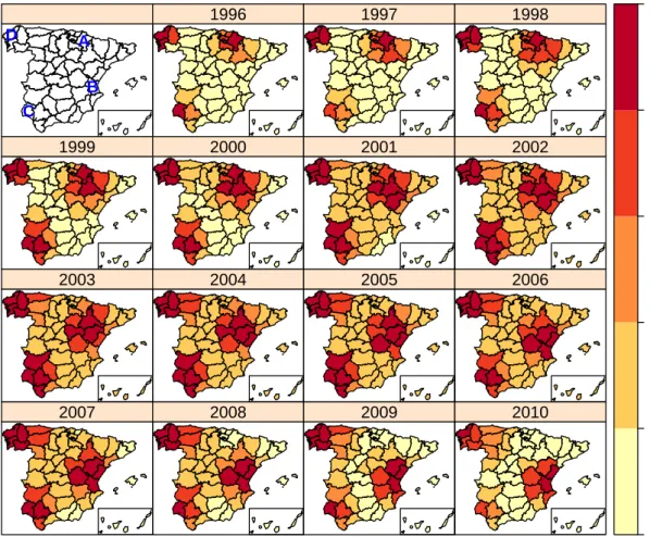
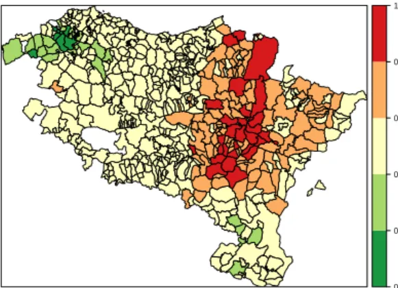
2.1 Geographical patterns of brain cancer mortality risks (top) and

sig-nificantly high risk provinces (bottom). . . 39

2.2 Overall temporal trends of brain cancer mortality risks. The X-axis represents years and the Y-axis givesexp(γ_t∗). . . 40

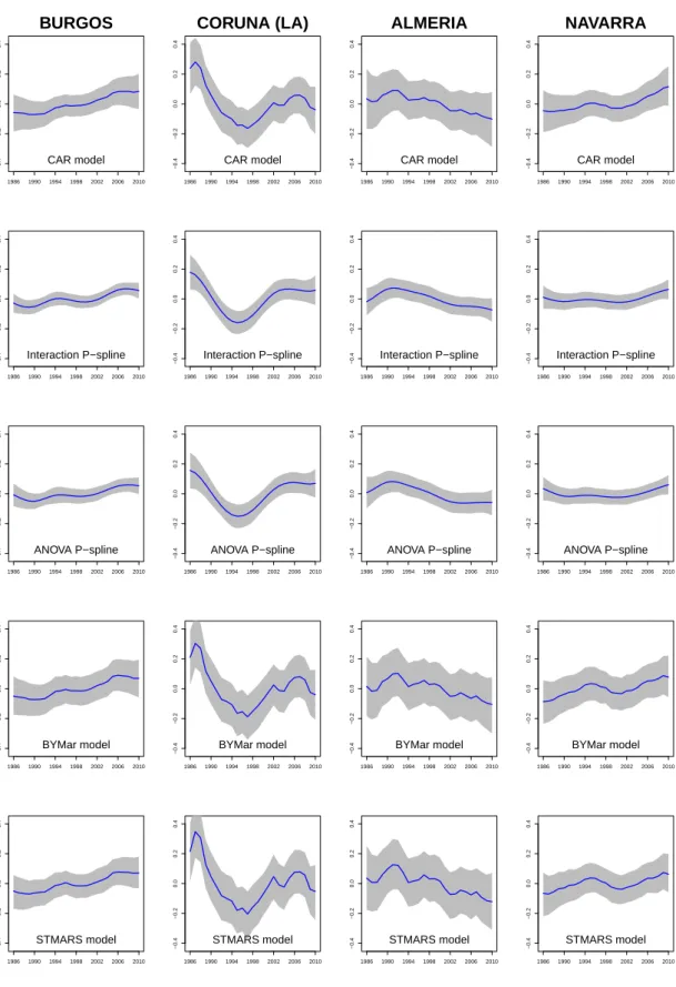
2.3 Spatio-temporal patternsδ_it∗ for each province. . . 41

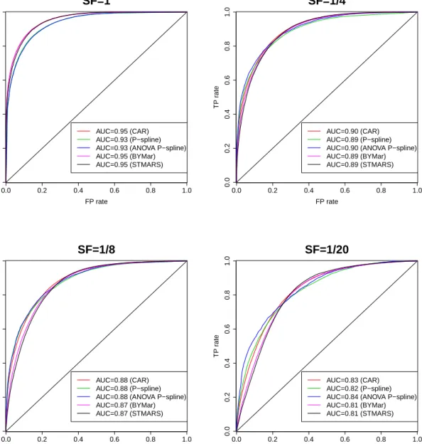
2.4 Scenario 1. AUC for different scale factor (SF) values. . . 45

2.5 Scenario 2: true risk surface. . . 46

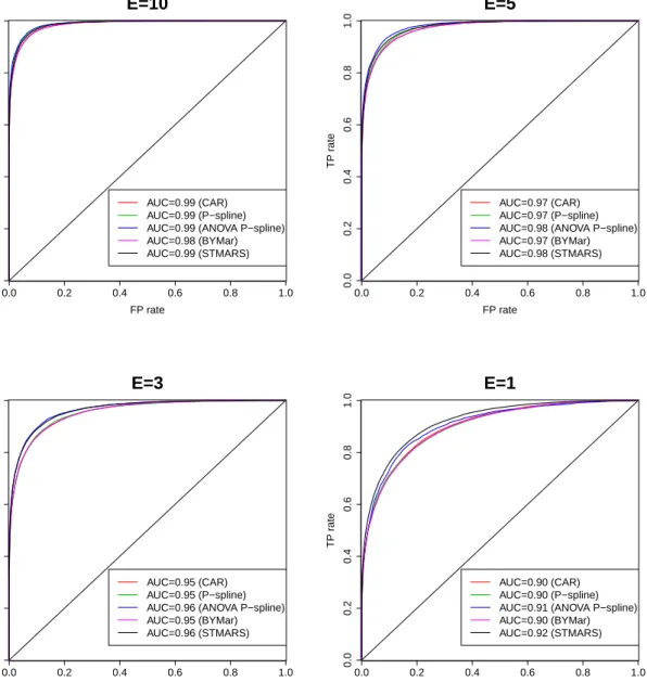
2.6 Scenario 2. AUC for different scale factor (SF) values. . . 49

3.1 Map of the n = 501 municipalities of Navarre and Basque Country. (a) Municipalities grouped in provinces; (b) Municipalities aggregated by SLAs. . . 56

3.2 Global spatial and temporal patterns in the analysis of brain cancer mortality in Navarre and the Basque Country. . . 59

3.3 Space-time interaction termδˆj(i)t for each health area. . . 60

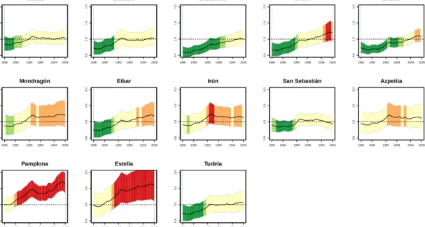
3.4 Temporal evolution of the estimated brain cancer mortality risks rˆit for the more populated municipalities of each heath area in Navarre and the Basque Country (Spain) and 95 % two-sided credible inter-vals. The red color indicates a high posterior probability of relative risks being greater than one. . . 60

3.5 Map of the municipality level spatial patterns of mortality risk (left) and global temporal pattern (right) in Scenario 1. . . 62

3.6 Province level space-time interactionsδj(i)tfor the generated log-risks surface in Scenario 1. . . 63

(12)

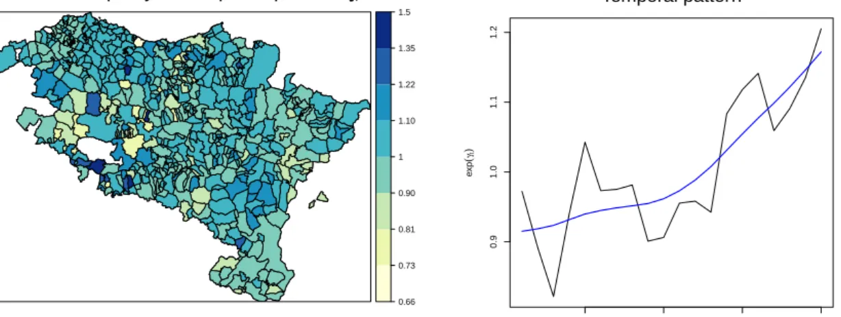
iv List of Figures 3.7 Map of the sum of municipality level ξi and basic health area level

ψj(i) spatial patterns of mortality risk (left) and SLA space-time

in-teractions δj(i)t (right) for the generated log-risks surface in Scenario 2. . . 64 3.8 Spatio-temporal true risk surface for the simulation study of Scenario

1 (top panel) and Scenario 2 (bottom panel). . . 65 4.1 Breast cancer mortality rates in Spanish provinces (per 100000 female

inhabitants). Period 1990-2010. . . 98 4.2 Spatial and temporal patterns of female breast cancer mortality

rel-ative risks in Spanish provinces. . . 101 4.3 Temporal evolutions of six selected Spanish provinces, exp(δ∗_it), and

95% two-sided credible intervals. The colors used in this figure are those associated to the legend of the map shown in Figure 4.2b but for P(exp(δ_it∗)>1). . . 102 4.4 Boxplots of the relative risk estimates for the spatially structured

one-dimensional temporal P-spline model (a), the temporally structured two-dimensional (anisotropic) spatial P-spline model with a Type II interaction (b), and the three-dimensional ANOVA-type P-spline model (c). . . 102 4.5 Map of the municipalities of Navarre and Basque Country (left) and

(13)

List of Tables

1.1 Specification and rank deficiency for the four possible types of space-time interaction proposed by Knorr-Held (2000). . . 10 1.2 Identifiability constraints for the spatio-temporal CAR models

de-scribed in Equation (1.4). . . 12 2.1 Approximated computational times (in seconds) for fitted models. . . 38 2.2 Scenario 1: average values of MARB and MRRMPSE for relative

risks and for spatial, temporal and spatio-temporal pattern estimates based on 100 simulated data sets. . . 43 2.3 Scenario 1: true and false positives rates using lower one-sided

credi-bility/confidence intervals. . . 44 2.4 Scenario 2: average values of MARB and MRRMPSE for relative

risks and for spatial, temporal and spatio-temporal pattern estimates based on 100 simulated data sets. . . 47 2.5 Scenario 2: true and false positives rates using lower one-sided

credi-bility/confidence intervals. . . 48 3.1 Main characteristics of all models described in Section 3.2. . . 54 3.2 Identifiability constraints for the space-time models including

two-level spatial random effects described in Section 3.2 and Type IV space-time interactions.. . . 55 3.3 Model comparisons in the analysis of brain cancer mortality data in

Navarre and the Basque Country. . . 57 3.4 Estimated posterior means and 95% credibility intervals for model

(14)

vi List of Tables 3.5 Average values of DIC, corrected DIC, logarithmic score (LS), root

mean squared errors (RMSE), mean absolute bias (MAB), average coverage percentages of the 95% credible interval for the risks, true positive rates (TPR) and false positive rates (FPR) in Scenario 1 and Scenario 2. . . 67 4.1 Specification of the different types of structure matrices and the prior

distribution over the regression coefficients of the interaction term fi(xt). . . 90 4.2 Identifiability constraints to fit one-dimensional temporal B-splines

or P-splines described in Equation (4.1). . . 91 4.3 Specification of the different types of structure matrices and the prior

distribution over the regression coefficients of the interaction term ft(x1,x2). . . 93

4.4 Identifiability constraints to fit two-dimensional B-splines or P-splines described in Equation (4.2). Here first order penalties for longitude and latitude are considered for P-splines. . . 94 4.5 Identifiability constraints to fit two-dimensional B-splines or P-splines

described in Equation (4.2). Here second order penalties for longitude and latitude are considered for P-splines. . . 95 4.6 Identifiability constraints for the ANOVA-type P-spline model. . . 97 4.7 Model selection criteria (DIC, DICc, WAIC and logarithmic score)

and computational time (in seconds) from fitted models in the analy-sis of breast cancer mortality data in Spain. Full Laplace approximation.100 4.8 Model selection criteria (DIC, DICc, WAIC and logarithmic score)

and computational time (in minutes) from fitted models in the anal-ysis of simulated data in the municipalities of Navarre and Basque Country. Simplified Laplace approximation. . . 105

(15)

Introduction

Disease mapping is an area of research of great interest in epidemiology and public health. The great variability inherent to classical risk estimation measures, such as the standardized mortality ratios (or crude rates), makes it necessary to use statistical techniques to stabilize those ratios. Many statistical models have been developed during the last years to study the geographical distribution of a disease and its evolution in time. However, the availability of high quality data recorded for many years and regions, and the emergence of new and increasingly sophisticated models, has brought new difficulties (large computing time and identifiability issues among others) that need to be thoroughly investigated. This dissertation is mainly developed within a fully Bayesian approach with the following main objectives.

The first goal is to provide a brief review of the literature in spatio-temporal disease mapping that is relevant to the research objectives of this dissertation. Some comments on the main statistical software used for model fitting and inference have been also included. In Chapter 1, the non-parametric model proposed by Knorr-Held (2000) is described in detail. Identifiability issues related to these models are also revised, and constraints to fix these problems are clearly stated. Chapter 1also provides some insight into a new technique for Bayesian inference based on integrated nested Laplace approximations (Rue et al., 2009). The technique is known as INLA and it provides reliable results in short computational time. It can be used in the free statistical softwareRthrough theR-INLApackage. Some of its most useful tools are also described.

The second objective of this dissertation is to compare some of the existing mod-els in the literature analyzing their smoothing effects (in both space and time), and evaluating their ability to detect high-risk areas. Five different spatio-temporal mod-els used in disease mapping have been compared in Chapter 2: the non-parametric models described by Knorr-Held (2000), a CAR-based model in space and

(16)

autore-2 Introduction gressive model in time proposed byMartínez-Beneito et al.(2008), a moving average model in space and an autoregressive model in time presented in Botella-Rocamora (2010), and three-dimensional P-spline models for spatio-temporal count data pro-posed by Ugarte et al. (2010b) and Ugarte et al. (2012a). To make the different terms of the models comparable, a decomposition of the estimated log-risks is com-puted by defining posterior spatial, temporal, and spatio-temporal “patterns”. The results are illustrated using male brain cancer mortality data in Spanish provinces during the period 1986-2010. A simulation study is also conducted to compare the performance of the models in terms of sensitivity (ability to detect true high-risk regions) and specificity (ability to discard false high-risk regions) in two different scenarios (one based on the results obtained from a CAR model and a model-free scenario).

The third objective is to solve identifiability issues in spatio-temporal disease mapping models. This is a transversal objective which will be be addressed through-out the whole dissertation. Particular attention is paid on the new model proposals of Chapter 3 and Chapter 4, where the necessary set of constraints are derived by reparameterizing the random effects using the spectral decomposition of their precision matrices (Goicoa et al., 2017).

The fourth objective is to propose a new family of spatio-temporal models in-cluding two-level spatial random effects, and allowing to model the spatial and spatio-temporal effects at different administrative aggregation levels (as for exam-ple, municipalities within provinces or health areas, or counties that are grouped in states affected by similar health policies). In Chapter 3 these new model propos-als are described and presented as natural extensions of the spatio-temporal CAR models (Knorr-Held, 2000). Brain cancer mortality data in the municipalities of Navarre and Basque Country during the period 1986-2008 is used to illustrate the results. In addition, a simulation study based on the analyzed municipality data is conducted to compare the single-level and two-level models in terms of smoothing and high-risk area detection. An appendix with both the identifiability constraints and the R code to fit these models with INLA has been included at the end of this chapter.

The fifth objective of this dissertation is to propose B-spline models in a fully Bayesian approach accounting for both the spatial and temporal correlation. In Chapter 4, different possibilities of modelling the space-time interaction using (pe-nalized or un-pe(pe-nalized) B-splines are proposed. If the interest relies on analyzing the temporal evolution of risks in small areas, fitting one-dimensional temporal B-splines for each area could be preferable. If the focus is on studying the evolution in time of the geographical distribution of the risks, two-dimensional spatial B-splines for each time point can be considered. Three-dimensional P-spline models in a fully Bayesian setting are also described, in contrast to Ugarte et al. (2010b) andUgarte

(17)

Introduction 3 et al.(2012a) that used these models in an empirical Bayes disease mapping setting. Breast cancer mortality data in continental Spain during the period 1990-2010 and a simulated data for the municipalities of Navarre and Basque Country are used to illustrate the results. An appendix with both the identifiability constraints and the R code to fit these models with INLA has also been included at the end of this chapter.

Finally, this dissertation ends with some conclusions and comments on further research lines.

(18)

(19)

1

Spatio-temporal disease mapping

1.1 Introduction

Models to describe the geographical distribution of a disease and its evolution in time are abundant in the spatio-temporal disease mapping literature. There has been a tremendous growth of statistical techniques for disease mapping in the last few years, mainly due to the availability of information from modern registers with high quality data recorded throughout many years and regions. The information provided by these analyses is crucial for health researchers as it helps to formulate hypothesis about the etiology of a disease and the main risk factors. Detecting hotspot areas is also of great interest for policy makers to plan effective prevention/intervention programmes.

The great variability inherent to classical risk estimation measures such as the standardized mortality ratio (SMR), makes necessary to use models that borrow strength from spatial and temporal neighbors in spatio-temporal disease mapping studies (see for example Ugarte et al., 2014). Research into spatial and spatio-temporal disease mapping has been carried out within a hierarchical Bayesian frame-work, with generalized linear mixed models (GLMM) playing a major role. Two main approaches have been followed for model fitting and inference, the empirical Bayes (EB) and the fully Bayes (FB) approach. Both approaches have been used in the literature and both have advantages and disadvantages (see Goicoa et al., 2012 for some discussion), but the FB approach has experienced an enormous expansion due to the advent of modern computers and free software to run Markov chain Monte Carlo (McMC) algorithms such as WinBUGS (Spiegelhalter et al., 2003), Open-BUGS (Lunn et al., 2009), JAGS (Plummer, 2016) and the new initiative STAN (Stan Development Team,2016).

The FB approach provides posterior marginal distributions of the target param-eters instead of a single point estimate. However, the posterior distributions are not

(20)

6 Spatio-temporal disease mapping usually available in closed form and McMC algorithms have to be used, a computer intensive simulation-based technique. Even though these methods are very general and can be applied to virtually any model providing exact inference, in practice these algorithms can lead to high Monte Carlo errors and large computation time due to the complexity of disease mapping models (Schrödle et al.,2011) and the high dimension of the data. Moreover, specific algorithms not implemented in available software are often needed (Schmid and Held,2004). Hence, a trade-off between exact inference, model complexity, and computing time has to be achieved. Additionally, the choice of priors for the hyperparameters is important to obtain reliable inference (see for example Wakefield,2007;Fong et al.,2010 for some discussion). In addition to McMC, an approximate method for Bayesian inference in latent Gaussian models has recently been developed byRue et al.(2009). The method uses integrated nested Laplace approximations (INLA) and numerical integration to estimate the posterior marginal distributions of the quantities of interest. Many latent Gaussian models admit conditional independence properties leading to sparse precision matrices, and INLA takes advantage of this to speed computation. This allows to make Bayesian inference without running long and complex McMC algorithms.

Model fitting and inference in the EB approach commonly rely on the well known penalized quasi-likelihood (PQL) technique. The maximum likelihood estimation of GLMM with counts usually requires numerical integration and PQL can reduce the problem to a series of weighted least squares regressions using a Laplace approxi-mation to the quasi-likelihood (see Breslow and Clayton,1993). Hence, it has been used in disease mapping as an alternative to McMC methods. It provides good point estimates for Poisson models (Dean et al.,2004), it is computationally simple and fast, and it has few convergence problems. However, it can be less accurate for binomial data, and inference relies on asymptotic distributions without clear guide-lines about when this theory provides accurate inference (see Breslow, 2004and the references therein for an in depth discussion about PQL). An additional drawback of PQL is that the variability due to the estimation of the variance components is not taken into account in the global computation of the risk variability, but some authors (see for example Ugarte et al., 2008) have developed a mean squared error estimator to avoid this limitation.

The literature about Bayesian spatio-temporal disease mapping is extensive. For example, Bernardinelli et al. (1995) use a spatio-temporal model with linear trend while Assunção et al. (2001) consider a second-degree polynomial trend model. Re-garding non-parametric models, the work byKnorr-Held(2000) proposing four types of space-time interactions deserves attention. Martínez-Beneito et al. (2008) focus on an autoregressive approach to spatio-temporal disease mapping, andUgarte et al. (2009a) compare the performance of different space-time models. Most of the re-search in disease mapping is based on conditional autoregressive priors (CAR) for

(21)

1.2 Spatio-temporal models for disease mapping 7 both spatial and temporal effects, extending the seminal work ofBesag et al.(1991). However, other approaches based on splines have been also developed. Within an EB approach,MacNab and Dean (2001) consider autoregressive local smoothing in space and B-spline smoothing for time. Ugarte et al. (2010b, 2012b) consider a pure interaction P-spline model for space and time, and Ugarte et al. (2012a) use an ANOVA type P-spline model to describe spatio-temporal patterns of prostate cancer mortality in Spain. From a FB approach, spline smoothing has also been used in disease mapping (see for example, MacNab, 2007; MacNab and Gustafson, 2007).

This dissertation is developed within a fully Bayesian approach, using the INLA estimation technique to obtain reliable results in short computational time. This technique can be easily used in the free statistical software R (R Core Team, 2017) using the R-INLA package. Most of the work in spatial and spatio-temporal dis-ease mapping with INLA considers the Besag et al. (1991) model (hereafter BYM model) which includes two spatial random effects: one assuming a Gaussian ex-changeable prior to model unstructured heterogeneity and another one assuming an intrinsic conditional autoregressive prior (iCAR) for the spatially structured vari-ability. See for example, Schrödle et al. (2011); Schrödle and Held (2011a); Held et al. (2010); Schrödle and Held (2011b) orBlangiardo et al. (2013). However, the iCAR prior is improper and has the undesirable large-scale property of tending to a negative pairwise correlation for regions located further apart (seeMacNab, 2011; Botella-Rocamora et al., 2013). In addition, the variance components in the BYM convolution model are not identifiable from the data (MacNab, 2014) and informa-tive hyperpriors are needed for posterior inference. In this dissertation, the prior proposed by Leroux et al. (1999) is considered to model the spatial effect. This prior has been shown to outperform the iCAR prior (Lee, 2011). The model can be implemented in R using the R-INLA package as shown inUgarte et al. (2014).

The rest of the chapter is organized as follows. InSection 1.2, the non-parametric model proposed by Knorr-Held (2000) is described in detail, where four types of space-time interactions can be considered to model area-specific temporal evolutions. The necessary set of identifiability constraints for each model are clearly established, which are derived by reparameterizing the random effects using the spectral decom-position of their precision matrices (Goicoa et al., 2017). In Section 1.3, the INLA estimation techniques for model fitting and inference is briefly described. Finally, the R-INLA package and some of its more useful tools are described in Section 1.4.

1.2 Spatio-temporal models for disease mapping

Suppose that the region under study is divided into n small areas labelled as i = 1, . . . , n. For each area i, data are available for different time periods labelled by

(22)

8 Spatio-temporal disease mapping t = 1, . . . , T. Then, conditional on the relative risk rit, the number of counts Oit is

assumed to be Poisson distributed with mean µit = eitrit, where eit is the number

of expected cases for area i and time t. That is

Oit|rit ∼ P oisson(µit =eitrit),

logµit = logeit+ logrit.

Here, logeitis an offset and depending on the specification oflogritdifferent models

are defined.

To compute the number of expected caseseit, both direct and indirect

‘age-and-sex’ standardization procedures can be performed (note that other standardization variables could also be used in addition to age or sex). The direct method uses a single standard population to compute the ‘age-and-sex’ adjusted rates for each area and time period, producing rates that these areas would have if they had the same age and sex distribution as the standard population. On the other hand, the indirect method uses the same ‘age-and-sex’ rates (generally those computed using the information from all the areas together along the whole study period) applied to the observed population in each small area and time point. The indirect standardization procedure has been considered in all the real data analyses presented in this dissertation, so that eit is computed as

eit = J X j=1 Nitj Oj Nj i= 1, ..., n; t= 1, ..., T,

where Oj and Nj are respectively the number of counts and the population size in

‘age-and-sex’ group j ∈ {1, . . . , J}, so that Oj = n X i=1 T X t=1 Oitj and Nj = n X i=1 T X t=1 Nitj.

Then, eit represents the number of cases we would expect if the areaiin time point

t behaves as the whole region during the studied period.

A wide range of spatio-temporal models for disease mapping has been proposed in the literature, most of them based on CAR models extending the well known BYM model (Besag et al., 1991). Probably, the parametric model with linear time trend proposed by Bernardinelli et al. (1995) and the non-parametric models including different types of space-time interactions described in Knorr-Held (2000) are the most used models in space-time disease mapping. In the parametric model proposed

(23)

1.2 Spatio-temporal models for disease mapping 9 byBernardinelli et al. (1995), the log-risks can be modelled as

logrit=η+ξi+ (β+ϕi)·t (1.1)

where η is an intercept, ξi is the spatial effect, β represents an overall linear time

trend and ϕi measures the deviation of area i from the global trend (also called

differential time trend). A modification of this model was used by Ugarte et al. (2014). These authors use the Leroux et al.(1999) CAR prior distribution (LCAR) for the spatial effect ξi instead of the originally proposed iCAR prior. That is, the

prior for the spatial random effects ξ = (ξ1, . . . , ξn)

0

is given by

ξ ∼N(0,[τξ(λξRξ+ (1−λξ)In)]−1), (1.2)

where λξ is a spatial smoothing parameter taking values between 0 and 1, In is

an identity matrix of dimension n×n, and Rξ is the n ×n spatial neighborhood

matrix with diagonal elements equal to the number of neighbors of each area and non-diagonal elements (Rξ)ij = −1 if areas i and j are neighbors and (Rξ)ij = 0

otherwise. Here, two areas are considered as neighbors if they share a common border. Note that when λξ = 0 the LCAR prior reduces to an exchangeable prior

ξ∼N(0, τ_ξ−1In), whereas the iCAR priorξ ∼N(0,[τξRξ]−)is obtained when λξ = 1. The symbol−denotes the Moore-Penrose generalized inverse of a matrix. For the differential trend ϕ = (ϕ1, . . . , ϕn)

0

, an exchangeable distribution ϕ ∼ N(0, τ−1

ϕ In)

or an iCAR prior distribution ϕ∼N(0,[τϕRξ]−) can be considered.

However, the assumption of a linear time trend may be very unrealistic in prac-tice, where it is common to observe more general temporal trends due to improve-ment in treatimprove-ments, screening and early detection programmes, and research ad-vances in general. A natural extension to Equation (1.1) is to drop out linearity and assume non-parametric trends. Slight modifications of the models proposed by Knorr-Held (2000) were considered byUgarte et al. (2014). There, the log-risks are modelled as

logrit =η+ξi+φt+γt+δit (1.3)

where η quantifies the logarithm of the global risk, ξi is the spatial component, φt

and γt represent the unstructured and structured temporal effects respectively, and

δit is the space-time interaction effect. Note that dropping the interaction terms

leads to additive models. All the components in Equation (1.4) can be modelled as Gaussian Markov random fields (GMRF) (see Rue and Held, 2005), and prior densities can be written according to some structure matrices. Again, the LCAR prior was considered for the spatial random effect ξ. The unstructured temporal random effectsφt were modelled as independent and identically distributed normal

random variables with mean 0 and precision τφ. That is, φ = (φ1, . . . , φT)

0

∼

(24)

10 Spatio-temporal disease mapping Table 1.1: Specification and rank deficiency for the four possible types of space-time interaction proposed by Knorr-Held (2000).

Space-time interaction Rδ

Rank deficiency of Rδ

RW1 prior forγ RW2 prior forγ

Type I In⊗IT − − Type II In⊗Rγ n 2n Type III Rξ⊗IT T T Type IV Rξ⊗Rγ n+T −1 2n+T −2 random effects γ = (γ1, . . . , γT) 0

, random walks of first (RW1) or second order (RW2) prior distributions were assumed, i.e., γ ∼ N(0,[τγRγ]−), where Rγ is the

T ×T structure matrix of a RW1/RW2.

The interaction random effect δ = (δ11, . . . , δ1T, . . . , δn1, . . . , δnT)

0

was assumed to follow the multivariate normal distribution δ ∼ N(0,[τδRδ]−), where Rδ is the

nT×nT matrix obtained as the Kronecker product of the corresponding spatial and temporal structure matrices (seeClayton,1996), where four types of interactions can be considered. In Type I interactions (Rδ =In⊗IT), all parameters δit are a priori

independent without any structure in space and time. In Type II interactions (Rδ= In⊗Rγ), eachδi· fori= 1, . . . , n, follows a random walk independent from all other regions; i.e., temporal trends are different from region to region, and do not have any structure in space. In Type III interactions (Rδ =Rξ⊗IT), eachδ·tfort = 1, . . . , T,

follows an independent iCAR prior distribution; i.e., different spatial distributions for each time point without any temporal structure are assumed. Finally, in Type IV interactions (Rδ = Rξ ⊗Rγ), each δit is completely dependent over space and

time. That is, different temporal trends are assumed from region to region, but trends from neighboring regions tend to be similar. The structure matrices for the different type of interactions and their rank deficiencies are summarized inTable 1.1. In practice, the temporal effect of the data is usually structured, so the uncorre-lated temporal component φt can be removed and the following model is considered logrit =η+ξi+γt+δit. (1.4)

In this model, identifiability problems arise because the overall level can be absorbed by both the spatial and time effects, and the interaction terms are confounded with the main effects. To ensure model identifiability, sum-to-zero constraints are usually imposed over the random effects of the model (see for example Knorr-Held, 2000; Schmid and Held,2004orSchrödle et al.,2011). Necessary identifiability constraints using RW1 or RW2 prior for the temporally structured random effect and different

(25)

1.3 Model fitting and inference 11 types of space-time interactions are summarized in Table 1.2. The details of how these sum-to-zero constraints solve the identifiability problems in spatio-temporal models are given in Goicoa et al. (2017). In this paper, the spatial, temporal, and spatio-temporal interaction random effects are reparameterized using the spectral decompositions of their precision matrices to establish the appropriate identifiability constraints, removing the combinations of the random effects that are in the span of the fixed effects (Reich et al., 2006; Hodges and Reich, 2010).

This procedure is briefly described in what follows. Let us consider a Gaussian random effect a ∼ N(0,[τQ]−), with precision matrix τQ. The spectral decompo-sition of Q is given by Q=UΣU0 = [Ur :Us] 0 0 0 Σe U0_r U0_s ,

where U = [Ur :Us] is an orthogonal matrix whose columns, Ur and Us, are the

eigenvectors of Q having null and non-null eigenvalues respectively, and Σe is a

diagonal matrix with the non-null eigenvalues of Q in the main diagonal. Then, as

Uis orthogonal, a=UU0a= [Ur :Us] U0_r U0_s a.

So, the random effect a can be reparameterized asa=Xβ_a+Zαa, where

X =Ur, βa =U 0 ra, and αa ∼N(0,[τΣ]e −1). Z=Us, αa=U 0 sa, (1.5)

Deleting the repeated columns obtained in the design matrices of the spatial, tem-poral, and spatio-temporal random effects of Equation (1.4) circumvents the iden-tifiability issues, which implies suitable sum-to-zero constraints (see Goicoa et al., 2017for details). The procedure will be used to derive the necessary constraints for the model proposals inChapter 3 and Chapter 4.

1.3 Model fitting and inference

Model fitting and inference in spatio-temporal disease mapping models have usually been done using either an empirical Bayes (EB) or fully Bayes (FB) approach. In the EB approach, penalized quasi-likelihood (PQL) has been widely used (see for example MacNab and Dean, 2001; Dean et al., 2004; Ugarte et al., 2008, 2009b, 2010b). From a FB perspective, usually Markov chain Monte Carlo (McMC) tech-niques have been used because the posterior distributions cannot be obtained in

(26)

12 Spatio-temporal disease mapping Table 1.2: Identifiability constraints for the spatio-temporal CAR models described in Equation (1.4).

Interaction RW1 prior forγ RW2 prior forγ

Type I n P i=1 ξi = 0, T P t=1 γt = 0, n P i=1 ξi = 0, T P t=1 γt= 0, n P i=1 T P t=1 δit= 0 n P i=1 T P t=1 δit= n P i=1 T P t=1 tδit= 0 Type II n P i=1 ξi = 0, T P t=1 γt = 0, n P i=1 ξi = 0, T P t=1 γt= T P t=1 tγt= 0, T P t=1 δit = 0, for i= 1, . . . , n T P t=1 δit= 0, fori= 1, . . . , n Type III n P i=1 ξi = 0, T P t=1 γt = 0, n P i=1 ξi = 0, T P t=1 γt= 0, n P i=1 δit= 0, fort = 1, . . . , T n P i=1 δit = 0, for t= 1, . . . , T Type IV n P i=1 ξi = 0, T P t=1 γt = 0, n P i=1 ξi = 0, T P t=1 γt= 0, T P t=1 δit = 0, for i= 1, . . . , n T P t=1 δit = 0, fori= 1, . . . , n n P i=1 δit= 0, fort = 1, . . . , T n P i=1 δit = 0, for t= 1, . . . , T

closed form (see for exampleBernardinelli et al.,1995;Knorr-Held and Besag,1998; Knorr-Held, 2000; Best et al., 2005; Martínez-Beneito et al., 2008 or Ugarte et al., 2009a). In the following section, the INLA methodology is shortly described, because this is the fitting technique that will be used in Chapter 3 and Chapter 4.

1.3.1 Integrated nested Laplace approximations (INLA)

The INLA approach recently proposed by Rue et al. (2009), is a deterministic al-gorithm for Bayesian inference based on integrated nested Laplace approximations. INLA is especially designed for latent Gaussian models (a subclass of structured additive regression models), which are flexible enough to be used in many

(27)

differ-1.3 Model fitting and inference 13 ent types of applications. See Rue et al. (2017) for a review of recent examples of applications using the R-INLA package.

In these models, the response variable y= (y1, . . . , yN)

0

is assumed to belong to an exponential family, where the mean µi is linked to a predictor νi trough a link

functiong(·), such that g(µi) = νi. The structure additive predictor νi is defined as

follows νi =η+ J X j=1 βjuji+ L X l=1 fl(zli) for i= 1, . . . , N. (1.6)

whereη is an intercept, the coefficientsβ ={β1, . . . , βJ} represents the linear effect

of some covariates u = (u1, . . . , uJ)

0

, and f = {f1(·), . . . , fL(·)} are unknown

func-tions of the covariatesz= (z1, . . . , zL)

0

. Note that a very flexible class of models are defined, since very different forms can be assumed for the unknown functions fl(·),

such as smooth and nonlinear effects of covariates, and temporal or spatial random effects among others.

The models described inSection 1.2 fit into this framework and are usually built as Bayesian hierarchical models with three stages. The first stage is the observa-tional modelπ(y|x), whereπ(·|·)denotes the conditional density andyis the vector of observations. We assume that yi are conditionally independent given the vector

of all the latent (non-observable) components of interest xand the vector of hyper-parameters θ, so the distribution of the N observations is given by the likelihood

π(y|x,θ) = N

Y

i=1

π(yi|xi,θ).

The second stage is the latent Gaussian fieldπ(x|θ), where a multivariate Gaussian prior with zero mean and precision matrixQis assumed forx. This precision matrix typically depends on the hyperparametersθ (third stage), which are not necessarily Gaussian. That is,x∼N(0,Q−1₍_θ₎₎ _{with density function given by}

π(x|θ) = (2π)−N/2|Q(θ)|1/2_exp −1 2x 0 Q(θ)x .

The components of the latent Gaussian field x are supposed to be conditionally independent with the consequence thatQ(θ)is a sparse precision matrix (Blangiardo and Cameletti, 2015, Chapter 4.7.1). Note that if the components xi and xj are

conditionally independent given all the other components x−ij, that is, if the joint

conditional distribution can be factorized as π(xi, xj|x−ij) = π(xi|x−ij)π(xj|x−ij),

thenQij(θ) = 0and vice versa (Rue and Held,2005, Chapter 2, Theorem 2.2). This

specification is known aslatent Gaussian Markov random field (GMRF). Therefore, numerical methods for sparse matrices can be used when making inference with

(28)

14 Spatio-temporal disease mapping GMRFs, which are much quicker than general algorithms for dense matrices.

Note that in the particular disease mapping model ofEquation (1.4), the latent Gaussian field is defined as x = (η,ξ0,φ0,γ0,δ0)0, while the unknown precision pa-rameters and the spatial smoothing parameter form the vector of hyperpapa-rameters θ = (τξ, λξ, τφ, τγ, τδ)

0

.

In the following, we briefly explain the approximate Bayesian inference strategy of INLA. For further details see Rue et al. (2009) or Blangiardo and Cameletti (2015). The main goal is to estimate the marginal posterior distributions for each element of the GMRF π(xi|y) = Z π(xi,θ|y)dθ= Z π(xi|θ,y)π(θ|y)dθ (1.7)

and for each element of the hyperparameter vector π(θk|y) =

Z

π(θ|y)dθ−k.

The key feature of the INLA approach is to construct nested approximations of Equation (1.7). To do that, it is necessary to computeπ(θ|y)(and then the relevant marginals π(θk|y)can be obtained), andπ(xi|θ,y), which is needed to compute the

marginal posteriors π(xi|y). For the first task, the Laplace approximation method

described in Tierney and Kadane (1986) can be used, so that the joint posterior density of the hyperparameters π(θ|y) is approximated as

˜ π(θ|y)∝ π(y|x,θ)π(x|θ)π(θ) ˜ πG(x|θ,y) x=x∗₍_θ₎_, (1.8)

where the denominator π˜G(x|θ,y) denotes the Gaussian approximation to the full

conditional distribution of x, and x∗(θ) is the mode for a given θ. To integrate out the uncertainty with respect to θ, it is essential to explore the properties of Equation (1.8) and find good evaluation points θk for a numerical integration of

Equation (1.7). This is done by an iterative algorithm (Rue et al., 2009). Addi-tionally, an appropriate area weight ∆k must be assigned to each θk. Details about

how posterior marginals π(θk|y) are computed using numerical integration of an

interpolant are available in Martins et al. (2013).

To compute the marginal distributionsπ(xi|θ,y), three different approaches are

possible: a Gaussian approximation, a full Laplace approximation, and a simplified Laplace approximation. In the Gaussian approximation, the posterior conditional distributionsπ(xi|θ,y)are directly approximated as the marginals fromπ˜G(x|θ,y).

This approximation is the fastest option and often gives accurate results in short computational time, but according toRue and Martino(2007) unsatisfactory results

(29)

1.4 The R-INLA package 15

can be obtained due to errors in the location of the posterior marginals, errors due to the lack of skewness or both. The approximation can be improved through applying another Laplace approximation to π(xi|θ,y) similar to the one described in

Equa-tion (1.8). However, this “full Laplace” strategy can be computationally expensive. That is the reason whyRue et al. (2009) develop the simplified Laplace approxima-tion based on a Taylor’s series expansion of the full Laplace approximaapproxima-tion. This method is less time consuming and gives accurate results in many applications.

Finally, an approximation to the posterior marginal density ofEquation (1.7) is given by ˜ π(xi|y) = X k ˜ π(xi|θk,y)˜π(θk|y)∆k.

1.4 The

R-INLA

package

The INLA methodology is implemented in the open sourceGMRFLib library written in C and Fortran (Martino and Rue, 2009). An interface with the free statistical software R (R Core Team, 2017), called R-INLA, is also available allowing model specification and fitting within R. The package can be downloaded and installed in

R by typing

> install.packages("INLA", repos="https://www.math.ntnu.no/inla/R/stable")

for the stable version, or

> install.packages("INLA", repos="https://www.math.ntnu.no/inla/R/testing")

for the testing version. To upgrade the package (type inla.version() to find out the currently installed version), use either the inla.upgrade(testing=TRUE) or

inla.upgrade(testing=FALSE)commands. Documentation for the package, many worked examples, and a discussion forum are also available in the R-INLA website

http://www.r-inla.org/.

As mentioned in the previous section, fixed effects, smooth and nonlinear terms, and random effects can be included in a formulaargument using thef() function. The interface is flexible enough to allow for the specification of different latent models and prior distributions for the hyperparameters (see Section 1.4.1 andSection 1.4.3 for details). We run the INLA algorithm with a call to the inla() function

> inla(formula, family=<family>, data=<data>, ...)

whereformulahas been previously defined, family is a string indicating the likeli-hood family1_{, and}_data_{is a data frame or list containing all the variables included in}

(30)

16 Spatio-temporal disease mapping the model. Many other additional arguments can be included into theinlafunction. See help(inla) for a complete list.

The output of the function is an object of class inla, a list containing all the results which can be explored with the names()function. By default, marginal dis-tributions for the latent field and for the hyperparameters are computed. In addition, the marginal posterior distribution of the linear predictor can be computed using the control.predictor=list(compute=TRUE)argument. Other features as the in-tegration strategy for π(θk|y) ("auto" (default), "ccd", "grid" or "eb") and the

approximation strategy for π(xi|θ,y) ("gaussian", "simplified.laplace"

(de-fault) or "laplace") can be also controlled within the control.inla=list(...)

argument.

Many examples of regression models, area and point-level spatial and spatio-temporal processes, as well as the corresponding R code for model fitting in R-INLA

can be found in Blangiardo and Cameletti (2015). In the following sections, a de-tailed description of someR-INLA(version 0.0-1480869339, dated 2016-12-04) model fitting tools described through this dissertation have been included.

1.4.1 Models for the latent Gaussian field

Many different latent models are implemented in the R-INLA package. The list of all available models can be obtained typing

> names(inla.models()$latent)

[1] "linear" "iid" "mec" "meb" [5] "rgeneric" "rw1" "rw2" "crw2" [9] "seasonal" "besag" "besag2" "bym" [13] "bym2" "besagproper" "besagproper2" "fgn" [17] "ar1" "ar" "ou" "generic" [21] "generic0" "generic1" "generic2" "generic3" [25] "spde" "spde2" "spde3" "iid1d" [29] "iid2d" "iid3d" "iid4d" "iid5d" [33] "2diid" "z" "rw2d" "rw2diid" [37] "slm" "matern2d" "copy" "clinear" [41] "sigm" "revsigm" "log1exp" "logdist"

For each model, a detailed description and usage examples are provided in http: //www.r-inla.org/models/latent-models. Some of them are briefly described in what follows. Assuming that x= (x1, . . . , xk)

0

is a vector of length k:

• The "iid" model defines an independent random Gaussian noise (or exchange-able) prior forx. That is

(31)

where τ is the precision parameter and Ik is the identity matrix of dimension

k×k. This model is specified inside thef() function as

> f(x, model="iid", ..., hyper=list(prec=list(...)))

• The "besag"model defines an intrinsic CAR prior for x. That is

x∼N(0,[τR]−),

whereτ is the precision parameter andRis thek×k spatial neighborhood matrix. This model is specified inside thef() function as

> f(x, model="besag", graph=<graph>, ..., + hyper=list(prec=list(...)))

where the spatial neighborhood matrix R is passed to the program through the

graph argument (an inla.graph object, a symmetric matrix or a filename con-taining the graph). By default, this model imposes the sum-to-zero constraint

Pk

i=1xi = 0 (constr=TRUE).

• The"bym"model defines theBYM (orconvolution) prior forxproposed byBesag et al.(1991). That is x=u+v; with u∼N(0,[τuR] −₎_, v∼N(0, τ_v−1Ik) where u = (u1, . . . , uk) 0

is the spatially structured component with precision pa-rameterτu (iCAR prior) and v= (v1, . . . , vk)

0

represents the unstructured spatial component with precision parameterτv (iid prior). This model is specified inside

the f()function as

> f(x, model="bym", graph=<graph>, ...,

+ hyper=list(prec.spatial=list(...), prec.unstruct=list(...)))

Since each data point is represented by two random effects, only their sum is identifiable. The "bym" model computes both the posterior distribution of u+v

(firstkelements), and the posterior distribution of the spatially structured effectu

(elements fromk+1to2k). By default, the sum-to-zero constraintPk

i=1(ui+vi) =

(32)

18 Spatio-temporal disease mapping

• The "rw1" model defines a first order random walk prior for x. It is constructed assuming independent increments

∆xi =xi−xi+1 ∼N(0, τ−1) fori= 1, . . . , k−1

whereτ is the precision parameter. This model is specified inside thef()function as

> f(x, model="rw1", ..., hyper=list(prec=list(...)))

By default, the sum-to-zero constraint Pk

i=1xi = 0 (constr=TRUE) is set.

• The"rw2"model defines asecond order random walk prior forx. It is constructed assuming independent second-order increments

∆2xi =xi−2xi+1+xi+1 ∼N(0, τ−1) for i= 1, . . . , k−2

whereτ is the precision parameter. This model is specified inside thef()function as

> f(x, model="rw2", ..., hyper=list(prec=list(...)))

By default, the sum-to-zero constraint Pk

i=1xi = 0 (constr=TRUE) is considered.

• The "generic0" model defines a generic prior for xsuch that

x∼N(0,[τC]−1),

where τ is the precision parameter and C is a structure (symmetric) matrix of dimensionk×kdefined by the user. This model is specified inside thef()function as

> f(x, model="generic0", Cmatrix=<Cmat>, ..., + hyper=list(prec=list(...)))

where the structure matrixCis passed to the program through theCmatargument (a dense or sparse-matrix).

• The "generic3" model defines a generic prior for xsuch that

x∼N  0, " _m X i=1 τiCi #−1 ,

(33)

whereτi is the specific precision parameter of the structure matrix Ci (of

dimen-sion k×k) defined by the user. This model is specified inside the f() function as

> f(x, model="generic3", Cmatrix=<list.Cmat>, ..., + hyper=list(prec1=list(...),prec2=list(...),...))

wherelist.Cmat is a list of length m (maximum 10) with the Ci matrices.

1.4.2 Implementing the LCAR prior

As already mentioned, the Leroux et al. (1999) CAR prior distribution is consid-ered in this dissertation for the spatial random effect. Recall that a LCAR prior distribution forx= (x1, . . . , xk)

0

is given by

x∼N(0,[τ(λR+ (1−λ)Ik)]−1),

where τ is the precision parameter, λ is the spatial smoothing parameter, R is the spatial neighborhood matrix of dimension k×k and Ik is an identity matrix.

This model was not originally available inR-INLA2, butUgarte et al.(2014) show how to built this prior distribution using the"generic1" model. According to the

R-INLA documentation, this model defines the following prior for x

x∼N 0, τ(Ik− β λmax C) −1! , (1.9)

whereτ is the precision parameter,Cis a structure (symmetric) matrix of dimension k×k defined by the user, and λmax is the maximum eigenvalue ofC, which allows

β to be in the rangeβ ∈[0,1). Let us define Cas C=Ik−R=    −ni+ 1, i=j 1, i∼j 0, otherwise (1.10)

whereni is the number of neighbors of the ith area. Ugarte et al.(2014) proves that

for this matrix λmax equals 1, so the covariance matrix defined in Equation (1.9)

2_{At the present time, an experimental version of the model is implemented under the name}

(34)

20 Spatio-temporal disease mapping takes the following expression

τ(Ik− β λmax C) −1 = [τ(Ik−β(Ik−R))] −1 = [τ(βR+ (1−β)Ik)] −1 ,

which matches the parameterization of the covariance matrix of the LCAR prior with β =λ. So, the LCAR prior can be specified inside the f()function as

> f(x, model="generic1", Cmatrix=<C.Leroux>, constr=TRUE, ..., + hyper=list(prec=list(...),beta=list(...)))

where C.Leroux is the structure matrix defined in Equation (1.10).

1.4.3 Prior distribution for the hyperparameters

Similar to the latent models, several prior distributions are implemented in R-INLA

for the hyperparameters θk. The list of all available priors can be obtained typing

> names(inla.models()$prior)

[1] "normal" "gaussian" "wishart1d" [4] "wishart2d" "wishart3d" "wishart4d"

[7] "wishart5d" "loggamma" "minuslogsqrtruncnormal" [10] "logtnormal" "logtgaussian" "flat"

[13] "logflat" "logiflat" "mvnorm" [16] "pc.ar" "none" "invalid" [19] "betacorrelation" "logitbeta" "pc.prec" [22] "pc.dof" "pc.cor0" "pc.cor1" [25] "pc.fgnh" "pc.spde.GA" "pc.matern" [28] "pc.range" "pc" "ref.ar" [31] "jeffreystdf" "expression:" "table:"

See the web page http://www.r-inla.org/models/priors for a detailed descrip-tion and examples of some of these priors. A novel approach using penalised com-plexity priors (PC priors) is described in Simpson et al. (2017).

In all the models for latent Gaussian fields described in Section 1.4.1, prior distributions for the precision parameters have to be specified. By default, log-Gamma distribution with parameters 1 and 5e-05 are given to the log-precision parameters in R-INLA, that is,

θ = logτ ∼logGamma(1,5e-05).

Note that for the "bym" model, the vector of hyperparameters is represented as

(35)

the spatially structured and unstructured components of the model. For the LCAR model described in Section 1.4.2, the vector of hyperparameters is represented as

θ= (logτ,logit(β)), with default hyperprior distribution

logit(β) = log β 1−β ∼N(0,0.1).

In addition to the prior distributions already implemented inR-INLA, the"table"

and"expression"priors allow the user to define any possible prior not implemented yet. Instead of using the default hyperpriors given by R-INLA, more suitable pri-ors have been implemented when analyzing real data examples in this dissertation. Specifically, an improper uniform prior distribution on the positive real line for the standard deviation, i.e., σ = 1/√τ ∼ U(0,∞); and a standard uniform distribu-tion for the spatial smoothing parameter, i.e., β ∼ U(0,1), have been defined for the hyperparameters of the random effects. However, INLA only allows to define an expression for the log-density θ1 = logτ in the first case and θ2 = logit(β) in

the second case. So, appropriate transformations are necessary to obtain equivalent distributions in each case.

Note that the σ ∼U(0,∞)prior distribution can be translated to an equivalent distribution on the log-precision scale, by making

π(θ1) = π(logτ) =π(σ) ∂σ ∂logτ ∝1· ∂exp(−logτ /2) ∂logτ ∝exp(−logτ /2), and it can be implemented in R-INLA as

> sdunif = "expression:

+ logdens = -log_precision/2; + return(logdens)"

Once the"sdunif"prior distribution has been defined, it can be included inside the

f()function as

> f(x, model=<model>, ..., hyper=list(prec=list(prior=sdunif)))

In a similar way, accounting for θ2 =logit(β) = log

β

1−β

, the density function of θ2 is expressed as π(θ2) =π(logit(β)) =π(β)· ∂β ∂θ2 =π(β)· exp(θ2) (1 + exp(θ2))2 =π(β)·β(1−β)

To define the standard uniform distributionβ ∼U(0,1)≡Beta(1,1), the log-density of π(θ2)can be implemented in R-INLA as

(36)

22 Spatio-temporal disease mapping > lunif = "expression: + a = 1; + b = 1; + beta = exp(theta)/(1+exp(theta)); + logdens = lgamma(a+b)-lgamma(a)-lgamma(b)+ + (a-1)*log(beta)+(b-1)*log(1-beta); + log_jacobian = log(beta*(1-beta)); + return(logdens+log_jacobian)"

Once the "lunif"prior distribution has been defined, it can be included inside the

f() function as

> f(x, model=<model>, ...,

+ hyper=list(beta=list(prior=lunif,initial=0)))

1.4.4 Posterior distribution of linear combinations

Depending on the context, it might be necessary to compute the posterior marginals for linear combinations of the elements in the latent field (‘fixed’ or ‘random’ effects) or for the linear predictor of the model. Details on how to compute these linear combinations within R-INLA are described in what follows.

For the first case, assume that our interest is in computing the posterior marginals of

w=Ax,

wherex= (x1, . . . , xk)

0

is the latent field andAis ap×k matrix wherepis the num-ber of linear combinations of the latent field. The functions inla.make.lincomb()

and inla.make.lincombs() can be used to define a linear combination or several linear combinations, respectively. As remarked in Martins et al. (2013), two dif-ferent approaches are provided in R-INLA. The first approach creates an enlarged latent field x˜ = (x,w) and then posterior marginals for x˜ are computed with the INLA method using the Gaussian, simplified Laplace or full Laplace approximation strategies described in Section 1.3.1. However, the addition of many linear combina-tions will lead to more dense precision matrices which will consequently slow down the computations. The second approach does not include w in the latent field, but performs a post-processing of the resulting output given by INLA and approximates the posterior marginals of w by a Gaussian distribution with

E[w|θ,y] =Aµ∗ and Var[w|θ,y] =A(Q∗)−1AT,

where µ∗ is the mean of the marginal approximationπ˜(xi|θ,y)and Q∗ is the

(37)

approach leads to a much faster approximation of the posterior marginals forwand that is why this is the default method inR-INLA. However, more accurate approxi-mations can be obtained switching to the first approach, if necessary, by including the following argument into the inlafunction

> inla(formula, family=<family>, data=<data>, ..., + control.inla=list(lincomb.derived.only=FALSE))

Spatial, temporal and spatio-temporal “patterns” are defined inSection 2.4as linear combinations of the linear predictor. Thus, the inla.make.lincombs()function is used to compute the posterior marginal distributions of these patterns.

However, as in the B-spline models proposed in Chapter 4, the response might depend on a linear combination of the latent field. Suppose that we want to fit the following model yi =η+ k X j=1 aijxi, for i= 1, . . . , N wherey= (y1, . . . , yN) 0

is the response vector,ηis an intercept,A= (aij)is a design

matrix of dimension N×k and x= (x1, . . . , xk)

0

is a vector of unknown coefficients where an exchangeable prior is considered, i.e., x ∼ N(0, τIk). This model can be

specified in R-INLA as

> # Define the formula argument

> formula <- y ~ -1 + intercept + f(x,model="iid",...) >

> # Call to the inla() function > eta <- rep(1,N)

> data <- list(intercept=c(1,rep(NA,k)),x=c(NA,1:k)) >

> inla(formula, family=<family>, data=data, ...,

+ control.predictor=list(A=cBind(eta,<A.matrix>),...))

where A.matrix contains the coefficients of the linear combinations. Internally,

R-INLA adds another layer in the hierarchical model ν∗ =Aν,

so that the likelihood function is linked to the latent field through ν∗ instead of ν, i.e., π(y|x,θ) = N Y i=1 π(yi|νi∗,θ).

(38)

24 Spatio-temporal disease mapping According toMartins et al.(2013), this feature is implemented by also adding ν∗ to the latent model, where the conditional distribution for ν∗ has the mean Aν and the precision matrix κAI, where the constant κA is set to a high value. In terms of

output from inla, the vector (ν∗,ν)will be the linear predictor.

1.4.5 Linear constraints for the latent Gaussian fields

In the spatio-temporal disease mapping models described inSection 1.2, sum-to-zero constraints are considered to ensure model identifiability between the intercept, the main spatial and temporal effects, and the space-time interaction effect.

In R-INLA, sum-to-zero constraints is the default option for intrinsic models (see Section 1.4.1) for the latent Gaussian field x, that is, Pk

i=1xi = 0. Including

this constraint (specified inside the f() function with theconstr=TRUE argument), makes it possible to identify the intercept and the main spatial/temporal effect. However, as stated in Table 1.2, additional contraints must be imposed over the spatio-temporal interaction term depending on its prior distribution. Using the

extraconstr argument, linear constrains such as Ax = b can be specified, where the number of rows of A is equal to the number of constraints to impose over x.

For example, let us consider the spatio-temporal model of Equation (1.4)where a RW1 prior is given to the temporal random effect γ = (γ1, . . . , γt)

0

, and a com-pletely structured prior (Type IV) is considered for the interaction effect δ = (δ11, . . . , δ1T, . . . , δn1, . . . , δnT)

0

. According to the Table 1.2, the following n +T sum-to-zero constraints on the interaction term are needed

T X t=1 δit= 0, for i= 1, . . . , n. n X i=1 δit = 0, fort = 1, . . . , T.

Note that these constraints can be written in the form Aδ =0 with

A= " In⊗1 0 T 10_n⊗IT # . (1.11)

The constraints are specified in the f()function as

> f(ID.delta, model="generic0", Cmatrix=<Cmat>,

+ rankdef=<rankdef>, constr=TRUE, hyper=list(prec=...), + extraconstr=list(A=<A.constr>, e=rep(0,<n.constr>)))

(39)

whereCmatis the Kronecker product of the spatial and temporal structure matrices,

rankdefis its rank deficiency, A.constris the (n+T)×nT dimension matrix given inEquation (1.11)andn.constris equal to the number of constraints to be imposed.

1.4.6 Model selection criteria

Criteria based on the deviance

When the interest is comparing different models in terms of model fitting and com-plexity, some criteria based of the deviance can be used. Given the data y with likelihood π(y|x,θ) the Bayesian deviance is defined as

D(x,θ) =−2 log{(π(y|x,θ)}+ 2 log{f(y)}. (1.12)

The deviance of the model is a measure that takes account of the variability associ-ated to the likelihood. Generally, the posterior mean devianceD(x,θ)is considered as a measure of goodness of it due to its robustness. However more complex models will fit better the data, and consequently lower values of the mean deviance will be obtained. The Deviance Information Criterion (DIC, Spiegelhalter et al., 2002) is the most commonly used measure of model fit based on the deviance for Bayesian models. The DIC is computed as the sum of the posterior mean of the deviance (a measure of goodness of fit) and the number of effective parameters (a measure of model complexity),

DIC=D(x,θ) +pD

where the quantity pD is defined as the posterior mean of the deviance minus the

deviance of the posterior means of the parameters of interest. Analogously to the Akaike information criterion (AIC), models with smaller DIC values provide better trade-off between model fit and complexity. To compute the DIC values, the op-tion control.compute=list(dic=TRUE) inside the inla() function is used. The details about how these quantities are computed in R-INLA can be found in Rue et al. (2009). It is very important to know that INLA does not compute the sat-urated deviance, i.e., the second term in Equation (1.12) is not used. In addition INLA, instead of evaluating the deviance at the posterior mean of all parameters, evaluates the deviance at the posterior mean of the parameters and at the posterior mode of the hyperparameters. The reason is that the posterior marginals for some hyperparameters (especially the precisions) might be highly skewed.

A corrected version of the DIC proposed by Plummer (2008) has been also con-sidered as model selection criterion, because it has been shown that DIC values may under-penalize complex models in disease mapping. The corrected DIC is defined

(40)

26 Spatio-temporal disease mapping as DICc=D(x,θ) + N X i=1 pDi/(1−pDi) (1.13)

where pDi is the contribution of observationi to the effective number of parameters

(see Spiegelhalter et al., 2002).

The more recently derived Watanabe-Akaike information criterion (Watanabe, 2010), also known as Widely Applicable Information Criterion (WAIC), which is recommended byGelman et al.(2014) over the DIC criterion, can be also computed by including the option control.compute=list(waic=TRUE). WAIC is a method for estimating pointwise out-of-sample prediction accuracy from a fitted Bayesian model, and unlike DIC, is invariant to parametrization and also works for singular models.

Criteria based on the predictive distribution

Different scoring rules can be defined to compare the models in terms of their pre-dictive performance by assigning a numerical score to each model based on their predictive distributions.

Given a set of spatio-temporal observations y= (y11, . . . , ynT)

0

, the logarithmic score (see Gneiting and Raftery,2007) is defined as

LS =− n X i=1 T X t=1 log(CPOit) (1.14)

where CPOit = P r(Yit = yit|y−it) values (conditional predictive ordinate, Pettit,

1990) denotes the cross-validated predictive probability mass at the observed count yit. The logarithmic score is asymptotically equivalent to the Akaike information

criterion if the observations are independent (Stone, 1977). Models with smaller resulting scores will be better in terms of predictive performance.

The probability integral transform (PIT,Dawid, 1984) for each observation can be also computed to assess the predictive quality of a model, which is defined as

PITit =P r(Yit≤yit|yit),

that is, the cross-validated predictive cumulative distribution at the observed count yit. If y comes from a continuous distribution, the PIT values have a standard

uniform distribution. So the histogram of the computed PIT values can be used as a diagnostic tool. U-shaped histograms indicate underdispersed predictive distri-butions, while hump or inverse U-shaped histograms point towards overdispersion. However, in the case of count data the predictive distribution is discrete and the

(41)

PITs are no longer uniform under the hypothesis of an ideal forecast. In this case, the adjusted version of the PIT suggested by Czado et al. (2009) can be used in-stead, although it is not recommended for binary responses or Poisson with very few counts.

As described by Rue et al. (2009), both CPO and PIT quantities are computed inR-INLA without re-running the model by including into the inla() function the argument control.compute=list(cpo=TRUE). Their accuracy in comparison with quantities that are obtained by McMC methods is discussed in Held et al. (2010). As noted in this paper, the approximation of the predictive measures might fail if the approximation of the latent field is not accurate enough. This is due to an insufficient exploration of the tail properties of involved densities. Hence, the full Laplace approximation might be obligatory to get reliable results. It is also possible to increase accuracy of the estimation for the tails of the marginal distributions by adding the option control.inla=list(strategy="laplace", npoints=<h>)

(42)

(43)

2

Evaluation of models for smoothing and

detecting high-risk areas: a comparison of

P-splines, autoregressive, and moving average

models

2.1 Introduction

Several models have been proposed for smoothing risks in disease mapping, consid-ering alternative ways of introducing both spatial and temporal dependence as well as spatio-temporal interactions. The non-parametric models proposed by Knorr-Held(2000) and described in Chapter 1, are possibly, the most widely used models in space-time disease mapping. However, other proposals have been also considered for smoothing risks. For example, Martínez-Beneito et al. (2008) propose CAR-based models in space and autoregressive models in time while Botella-Rocamora (2010) consider moving average models in space and autoregressive models in time. Lately, three dimensional P-spline models have been also used to smooth risks in space and time (Ugarte et al., 2010b, 2012a). Despite the fact that CAR and P-spline models have been compared in a spatial context (Goicoa et al., 2012), no comparisons have been performed in the spatio-temporal setting yet.

The aim of this chapter is to deal with this issue providing practitioners some guidance on choosing the most appropriate model in a particular situation. Brain cancer mortality data in Spanish provinces during the period 1986-2010 (already analyzed in Ugarte et al., 2014) will be used for illustration purposes. The main spatial, temporal and spatio-temporal patterns will be investigated. A simulation study will be performed to compare these models in different spatio-temporal sce-narios in terms of bias, variability, sensitivity (ability to detect true positives, i.e., ability to detect true high risk regions), and specificity (ability to discard false

(44)

pos-30 Evaluation of models for the detection of high-risk areas itives, i.e, ability to discard false high risk regions). Identifiability issues have been taken into account when fitting the previous models, considering the corresponding constraints for each one. In addition, an adequate decomposition of the log-risks is proposed to compare the patterns induced by all the models.

This chapter is laid out as follows. In Section 2.2 a brief review of P-spline models in spatio-temporal disease mapping is given, while Section 2.3 describes the autoregressive and moving average models mentioned above. Computational issues about model estimation and a decomposition of the estimated log-risks are detailed in Section 2.4. Brain cancer mortality data in Spanish provinces are ana-lyzed inSection 2.5 using all the models. Section 2.6 evaluates the capability of the models to detect true high risk areas performing a simulation study in two different spatio-temporal scenarios. Finally,Section 2.7concludes with a discussion and some interesting guidelines.

2.2 P-splines in spatio-temporal disease mapping

Although splines have become popular in a spatio-temporal context, their use has been mainly limited to model temporal rather than spatial effects (MacNab and Dean,2001;MacNab,2007;MacNab and Gustafson,2007). An anisotropic and non separable three-dimensional model is proposed in Ugarte et al. (2010b), extending the two-dimensional P-spline model proposed by Lee and Durbán (2009) to smooth risks in space and time. An ANOVA-type P-spline model was also considered in Ugarte et al. (2012a), allowing different smoothing parameters for the main spatial, temporal and interaction effects. In what follows, these three-dimensional P-spline models will be briefly described. See for example Goicoa et al.(2016) for a review of P-splines with B-splines bases in spatial and spatio-temporal disease mapping.

2.2.1 Interaction P-spline model

In the Interaction P-spline model (Ugarte et al., 2010b), the log-relative risks are modeled as a smooth function of the covariates

logrit =η+f(x1i, x2i, xt), for

i= 1, . . . , n,

t= 1, . . . , T, (2.1) where η is an intercept, x1i and x2i are the coordinates of the centroid of the area i

(longitude and latitude respectively),xtis the time, andf(x1i, x2i, xt)is an unknown

smooth function that is assumed to be sufficiently well approximated using P-splines with B-splines bases (Eilers and Marx, 1996).

In matrix form

Hierarchical and spline-based models in space-time disease mapping

PhD Thesis