The impact of precipitation physical processes on the polarimetric radar variables

(1)

UNIVERSITY OF OKLAHOMA GRADUATE COLLEGE

THE IMPACT OF PRECIPITATION PHYSICAL PROCESSES ON THE POLARIMETRIC RADAR VARIABLES

A DISSERTATION

SUBMITTED TO THE GRADUATE FACULTY in partial fulfillment of the requirements for the

Degree of

DOCTOR OF PHILOSOPHY

By

MATTHEW ROBERT KUMJIAN Norman, Oklahoma

(2)

THE IMPACT OF PRECIPITATION PHYSICAL PROCESSES ON THE POLARIMETRIC RADAR VARIABLES

A DISSERTATION APPROVED FOR THE SCHOOL OF METEOROLOGY

BY

______________________________ Dr. Alexander V. Ryzhkov, Co-Chair ______________________________ Dr. Howard B. Bluestein, Co-Chair ______________________________ Dr. Dušan S. Zrnić ______________________________ Dr. Alan Shapiro ______________________________ Dr. Guifu Zhang ______________________________ Dr. Eric R.I. Abraham

(3)

(4)

Acknowledgements

I want to express my gratitude to the members of my doctoral committee, who have dealt with numerous meetings, endless paperwork, and a number of inconveniences without complaints: Alexander Ryzhkov, Eric Abraham, Howie Bluestein, Alan Shapiro, Guifu Zhang, and Dušan Zrnić.

I thank Prof. Guifu Zhang for all the help and encouragement he’s given me over the past 6 years. He has always been supportive (and always thought I should have finished within a year or two of starting…). In addition, he provided me the valuable opportunity to teach in his courses, the fun experience of collecting hail, and, of course, several outstanding home-cooked Chinese meals.

Professor Alan Shapiro is a true mentor whose advice has been unwaveringly objective and honest, and whose infectious cynicism is a great source of wisdom and entertainment. I will never forget the camping trips and their valuable life lessons (“There is no such thing as too much garlic”), which I hope to remain a part of! The infamous Grill Fests were the highlights of the semesters. Prof. Shapiro is also one of the few who will show up at a dive bar on a Wednesday night (“F-5 IPA, yeaaa gotta have it!”) to hang out with the students, which leaves indelible impressions on all of us.

I thank Professor Eric Abraham for the encouragement and advice given over the years, dating back to our undergraduate physics late-night “help sessions.” He has provided some of the best school and career advice I’ve received, and I highly value his service as outside member on my committee. I hope to make a positive impression on my students as he did for me.

(5)

gratitude to Prof. Howie Bluestein. I appreciate his advice and encouragement over the years. When I was a youngster, his appearance in popular books on weather and storms served as an inspiration for me and got me thinking about the University of Oklahoma. I look forward to seeing him in Boulder next year for an excursion “through the melting layer”.

There is much that can be said about the legend himself, Dr. Dušan Zrnić. I am grateful and honored to have been a part of his research group, and for continually making his presence known. I will miss our philosophical talks about all topics, ranging from the meaning of the universe to Gilgamesh, and from the absurdities of some religious beliefs to the meaning of being a Professor. He made life in the cubicle enjoyable and entertaining, and his encouragement and helpful suggestions over the years are very much appreciated.

It is impossible to fully express my gratitude to Alexander Ryzhkov, whose guidance, understanding, and mentorship have profoundly influenced my life for the better. Working with him was the best thing that happened for my graduate studies. The number of opportunities he’s given me is incredible, and for this I am thankful. I have learned so much from his leadership and teaching, both in the realms of science (e.g., his profound influence on my academic career) and in life (e.g., the Три Заповеди Российского Зэка; see Appendix B). I strive to be able to one day achieve his level of scientific expertise, and I hope to pass on to future generations of scientists the positive influence he’s had on me. I look forward to our future collaboration and conversations!

Aside from my committee, there are numerous friends and colleagues that have been helpful in innumerable ways. I am thankful for the useful discussions and support

(6)

from David Parsons, Evgeni Fedorovich, Kelvin Droegemeier, and Yoshi Sasaki at SoM. I thank the rest of the RRDD group at NSSL (past and present): Valery Melnikov, Terry Schuur, Sebastián Torres, Dick Doviak, Pam Heinselman, Joey Picca, Jelena Andrić, Doug Forsyth, and Tonia Rollins. Great thanks to the “tool maker,” John Krause, whose code was used to produce many of the images presented in this dissertation. At ARRC, I’ve enjoyed my discussions and time with David Bodine, Bob Palmer, Tian Yu, Phil Stepanian, JoAnn Mehl, Krysta Bruehl, Phil Chilson, Jim Kurdzo, Boon Leng Cheong, and Qing Cao. I’d also like to express my thanks to Dan Dawson, Mike French, Jeff Snyder, Mike Buban, Kiel Ortega, Chris Schwarz, Dan Betten, Jana Houser, and the many others with whom I’ve spent fun times and had useful discussions. Thanks to the SoM “moms”, without whom I would still be lost: Celia Jones, Marcia Pallutto, Nancy Campbell, and Becky Steely. I am deeply grateful to Alex Schenkman, Charlotte Wainwright, and Scott and Michelle Ganson for their support and friendship, and for the many (many) hours we’ve spent together; I’ve enjoyed every moment of it.

Funding for this work comes from NSF Grant ATM-0532107; NOAA/OAR under NOAA/OU Cooperative Agreements #NA17RJ1227 and #NA11OAR4320072, U.S. Dept. of Commerce; Agreement 7000132024 with the MIT Lincoln Laboratory; and my doctoral fellowship from the University of Bonn, funded by the Deutsche Forschungsgemeinschaft (DFG) as part of the Transregional Research Center on “Patterns in Landsurface-Vegetation-Atmosphere Interactions” (TR32). Data from BOXPOL are courtesy of Meteorologisches Institüt der Universität Bonn, with thanks to Clemens Simmer, Silke Trömel, and Malte Diederich. OU-PRIME is owned and

(7)

operated by the Atmospheric Radar Research Center at the University of Oklahoma. Research-grade polarimetric radar data from KOUN are possible because of the tireless efforts of CIMMS/NSSL engineers and scientists who maintained and operated the radar. I’d also like to thank Pengefi Zhang and Dan Suppes, for their help in teaching me how to obtain, convert, and display polarimetric radar data from upgraded WSR-88Ds.

Finally, it is with the unwavering love, support, and encouragement from my family that I was able to achieve my doctorate. They have always been my greatest supporters and have never questioned my crazy idea to move to Oklahoma for nearly a decade to pursue study of my childhood fascination with the sky. Thank you so very much for everything that you have done for me.

(8)

List of Tables

Table 5.1: Fall speed relations used in Fig. 5.1. In each equation, D is in mm and the fall speed is in m s-1. ... 122 Table 6.1: Results of simulated evaporative changes in the polarimetric variables at S and C bands from the three soundings in Fig. 6.9. Simulations used the MP distribution with a rainfall rate aloft of 5 mm hr-1. ... 195 Table 6.2: As in Table 1, but the and distributions are used, respectively, the values resulting from each DSD model separated by a comma in the table. Magnitudes of Δρhv less than 10-4

are indicated as ≈0. ... 196 Table 6.3: Evaporative change in rainfall rate for each of the three soundings for the three rainfall algorithms R(ZH), R(ZH,ZDR), and R(KDP) (eqns. 6.34 – 6.36, respectively) based on the MP DSD along with the “true” rainfall rate calculated from the actual DSD. ... 198 Table 8.1: Explanation of symbols used throughout the equations and the text. ... 258

(13)

List of Figures

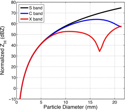
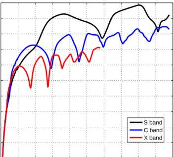
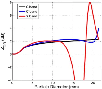
Fig. 1.1: Geometry of scattering.. ... 6 Fig. 1.2: View of the polarization plane (blue circle) illuminating a raindrop canted within the plane of polarization at angle α. The direction of wave propagation k is into the page. The raindrop’s major and minor axes (yellow arrows) are in the and directions, respectively. ... 8 Fig. 1.3: Shape factors and for oblate (top panel) and prolate (bottom panel) spheroids. ... 12 Fig. 1.4: Geometry of the two-layer spheroid, with an inner spheroid of dielectric constant 1 and outer dielectric 2. The silhouette of the inner spheroid is shown by the gray dashed curve. ... 12 Fig. 1.5: Schematic illustrating propagation effects of differential propagation phase shift and attenuation. Each panel shows successive times; the vertically-polarized signal is represented by the orange arrow, and the horizontally-polarized signal by the blue arrow, and propagation direction is given by the black vector, . The gradual separation of the H and V signals as they propagate through the rain represents the differential propagation phase shift. Signal amplitude is portrayed by the color shading of the arrows: the fading of the arrows represents attenuation. ... 21 Fig. 1.6: Schematic illustrating the depolarization of the incident electromagnetic wave as a result of hydrometeor canting. (a) The canted raindrop, characterized by major axis b and minor axis a (depicted by the yellow arrows) is illuminated by an incident horizontally-polarized wave depicted by the glowing green arrow. Because there is a component of the incident wave that is aligned with both axes of the drop (black dashed line), (b) both dipoles of the drop are excited, as depicted by the orange glowing arrows. (c) These excited dipoles emit secondary radiation that can be decomposed into horizontal and vertical components (the green dashed lines indicate the decomposition of the radiation emitted by the major axis b, and the cyan lines represent the decomposition of the radiation emitted by the minor axis a). (d) The scattered radiation in the forward and backward directions now has a cross-polar (vertically-polarized) component. ... 22 Fig. 1.7: Special cases where analytical formulas exist for the angular moments: (a) Completely random particle orientation, (b) random orientation in the horizontal plane, (c) two-dimensional axisymmetric Gaussian distribution of canting angles. In each case, the gray shaded regions represent the space of possible particle orientations. ... 31 Fig. 2.1a. Normalized radar reflectivity factors at orthogonal polarizations (H in blue, V in black) for (a) S (λ = 10.97 cm), (b) C (λ = 5.40 cm), and (c) X (λ = 3.2 cm) bands. Solid curves represent drop temperatures of 0 C; dashed curves represent drop temperatures of 20 C. ... 35

(14)

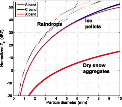
Fig. 2.1b: Normalized radar reflectivity factor at horizontal polarization (ZH) for raindrops, shown for S band (black), C band (blue), and X band (red) at two temperatures: 0 °C (solid curves) and 20 °C (dashed curves). ... 36 Fig 2.2: Normalized reflectivity factor at horizontal polarization (ZH) for raindrops (dotted lines) and ice pellets (solid lines), shown for S, C, and X bands (black, blue, and red curves). Ice pellets are considered the same size and shape as raindrops, but have a distribution of canting angles σ = 40°. ... 37 Fig. 2.3: Normalized reflectivity factor at horizontal polarization (ZH) for dry, oblate (axis ratio = 0.8, σ = 40_°) hailstones, at S, C, and X bands (black, blue, and red curves). ... 38 Fig. 2.4: Normalized reflectivity factor at horizontal polarization (ZH) for dry snow (thick curves), ice pellets (thin curves), and raindrops (dotted curves), at S, C, and X bands (black, blue, and red curves). Dry snowflakes are assumed to be oblate spheroids with axis ratio of 0.6, with density given by the empirical formula of Brandes et al. (2007). ... 39 Fig. 2.5: Normalized reflectivity factor at horizontal polarization (ZH) for melting snowflakes, shown for S, C, and X bands (black, blue, and red curves). Melting snowflakes treated using the model of Ryzhkov et al. (2008) and Giangrande (2007), at the level of the ZDR maximum in the brightband... 40 Fig. 2.6: Normalized reflectivity factor at horizontal polarization (ZH) for wet hailstones, shown for S, C, and X bands (black, blue, and red curves). Melting hailstones are treated using the model of Ryzhkov et al. (2009), at the ground level. ... 41 Fig. 2.7: Comparison of the oblate spheroidal shapes of a French-style dinner roll (left panel) to a 6-mm raindrop (right panel). Raindrop photograph adapted from Thurai et al. (2009). ... 44 Fig. 2.8: Differential reflectivity (ZDR) for raindrops at S, C, and X bands (black, blue, and red curves). Shown for two temperatures: 0 °C (top) and 20 °C (bottom). ... 44 Fig. 2.9: Differential reflectivity (ZDR) for frozen raindrops (ice pellets), shown for S, C, and X bands (black, blue, and red curves, respectively). Particle axis ratios are identical to those of raindrops; the width of canting angle distribution  = 40... 45 Fig. 2.10: Differential reflectivity (ZDR) for dry hailstones, at S, C, and X bands (black, blue, and red curves). The aspect ratio of hailstones > 1 cm in diameter is fixed at 0.8. ... 46 Fig. 2.12: Differential reflectivity (ZDR) for melting snowflakes, at S, C, and X bands (black, blue, and red curves). ... 49

(15)

Fig. 2.13: Observed vertical cross section (RHI) of ZH (left) and ZDR (right) showing a melting layer bright band between about 2.5 and 3.0 km in height. The data are from the Bonn X-band Polarimetric (BOXPOL) radar, collected on 22 June 2011 at 1144 UTC. Courtesy of the Meteorologisches Institüt at the Universität Bonn. ... 50 Fig. 2.14: Differential reflectivity (ZDR) for wet hailstones, for S, C, and X bands (black, blue, and red curves). ... 51 Fig. 2.15: Normalized specific differential phase shift (KDP) for raindrops, at S, C, and X bands (black, blue, and red curves). Shown for two temperatures: 0 °C (top) and 20 °C. ... 53 Fig. 2.16: Normalized specific differential phase shift (KDP) for ice pellets, at S, C, and X bands (black, blue, and red curves). ... 55 Fig. 2.17: Normalized specific differential phase shift (KDP) for dry hailstones, at S, C, and X bands (black, blue, and red curves). ... 55 Fig. 2.18: Normalized specific differential phase shift (KDP) for melting snowflakes, at S, C, and X bands (black, blue, and red curves). ... 57 Fig. 2.19: Normalized specific differential phase shift (KDP) for wet hailstones, at S, C, and X bands (black, blue, and red curves). ... 58 Fig. 2.20: Display of (top) ZH and (bottom) ρhv from the polarimetric WSR-88D radar in Key West, Florida (KBYX) on 7 February 2012, at 2128 UTC. Data show chaff mixed with precipitation. The chaff is clearly identified by ρhv as bands of extremely low ρhv values (< 0.70), whereas the precipitation has ρhv near unity. ... 62 Fig. 2.21: Display of (top) ZH and (bottom) ρhv from the polarimetric WSR-88D radar in Melbourne, Florida (KMLB) on 31 January 2012, at 2114 UTC. Data show a large grassfire north of the radar. The smoke and ash from the fire is clearly identified by ρhv values (< 0.50), whereas the clouds have ρhv near unity. ... 63 Fig. 2.22: Display of (top) ZH and (bottom) ρhv from the polarimetric WSR-88D radar in Huntsville, AL (KHYX) on 3 March 2012, at 0545 UTC. Data show a widespread region of biological scatterers, including insects and birds as very low ρhv, as well as a few precipitation cells evident by ρhv near unity. ... 64 Fig. 2.23: Display of (top) ZH and (bottom) ρhv from the polarimetric WSR-88D radar in Langley Hill, Washington (KLGX) on 7 February 2012, at 2242 UTC. Data show sea clutter mixed with precipitation. The sea clutter is clearly identified by ρhv values (< 0.70), whereas the precipitation has much higher ρhv (> 0.90). ... 65 Fig. 2.24: Display of (top left) ZH, (top right) Doppler velocity, (bottom left) ρhv, and (bottom right) ZDR from the polarimetric WSR-88D radar in Springfield, Missouri

(16)

(KSGF) on 29 February 2012, at 0605 UTC. Data show a tornadic debris signature, marked by high ZH, low ZDR, very low ρhv collocated with a vortex signature in the Doppler velocities, located at approximately x = 22 km, y = 39 km. ... 66 Fig. 2.25: Display of ρhv from the BOXPOL radar. Data are from the same scan as Figure 2.13. A dramatic decrease in ρhv is evident in the melting layer. The decrease in ρhv with range is a result of decreased signal-to-noise ratio, and possibly of nonuniform beam filling. ... 67 Fig. 2.26: Backscatter differential phase shift (δ) for raindrops, at S, C, and X bands (black, blue, and red curves). Shown for two temperatures: 0 °C (top) and 20 °C (bottom). ... 69 Fig. 2.27: Backscatter differential phase shift (δ) for ice pellets, at S, C, and X bands (black, blue, and red curves). ... 70 Fig. 2.28: Backscatter differential phase shift (δ) for dry hailstones, at S, C, and X bands (black, blue, and red curves). ... 70 Fig. 2.29: Backscatter differential phase δ for melting snowflakes at S, C, and X bands (black, blue, and red curves). ... 72 Fig. 2.30: As in Figure 2.13, but is shown. Note the “bump” in through the melting layer, caused by backscatter differential phase off large, wet snow aggregates. ... 73 Fig. 2.31: Schematic illustrating the difficulty estimating KDP (the slope of the dashed straight lines) in the presence of a δ bump on the radial profile of the measured (blue curve). Erroneously large positive and negative errors in the KDP estimates are depicted in red, whereas the true KDP is shown in green. ... 73 Fig. 2.32: Backscatter differential phase shift (δ) for melting hailstones, at S, C, and X bands (black, blue, and red curves). ... 74 Fig. 2.33: Linear depolarization ratio (LDR) for raindrops, at S, C, and X bands (black, blue, and red curves). Shown for two temperatures: 0 °C (top), and 20 °C (bottom). ... 76 Fig. 2.34: Linear depolarization ratio (LDR) for ice pellets, at S, C, and X bands (black, blue, and red curves). ... 77 Fig. 2.35: Linear depolarization ratio (LDR) for dry hailstones, at S, C, and X bands (black, blue, and red curves). ... 77 Fig. 2.36: Linear depolarization ratio (LDR) for dry snowflakes, at S, C, and X bands

(17)

Complex scattering amplitudes were computed using the Rayleigh approximation. The canting angle distribution width σ = 40°. ... 78 Fig. 2.37: Linear depolarization ratio (LDR) for melting snowflakes, at S, C, and X bands (black, blue, and red curves). ... 79 Fig. 2.38: Linear depolarization ratio (LDR) for wet hailstones, at S, C, and X bands (black, blue, and red curves). ... 80 Fig. 2.39: Normalized specific attenuation (AH) for raindrops at S, C, and X bands (black, blue, and red curves). Shown for two temperatures: 0 °C (top), and 20 °C (bottom). ... 83 Fig. 2.40: Normalized specific attenuation (AH) for ice pellets, at S, C, and X bands (black, blue, and red curves). ... 84 Fig. 2.41: Normalized specific attenuation (AH) for dry hailstones, at S, C, and X bands (black, blue, and red curves). ... 85 Fig. 2.42: Normalized specific attenuation (AH) for melting snow, at S, C, and X bands (black, blue, and red curves). ... 86 Fig. 2.43: Normalized specific attenuation (AH) for wet hail, at S, C, and X bands (black, blue, and red curves). Note that it is the same scale as for dry hailstones. ... 86 Fig. 2.44: Specific differential attenuation (ADP) for raindrops, at S, C, and X bands (black, blue, and red curves). Shown for two temperatures: 0 °C (top), and 20 °C (bottom). ... 88 Fig. 2.45: Specific differential attenuation (ADP) for ice pellets, at S, C, and X bands (black, blue, and red curves). ... 89 Fig. 2.46: Specific differential attenuation (ADP) for dry hailstones, at S, C, and X bands (black, blue, and red curves). ... 89 Fig. 2.47: Specific differential attenuation (ADP) in melting snowflakes at S, C, and X bands (black, blue, and red curves). ... 91 Fig. 2.48: Data from a vertical cross section through a winter stratiform precipitation event on 27 January 2009 at 2317 UTC, taken with the S-band KOUN along the 181° azimuth. The radial streak of negative ZDR emanating from about 50 km range is caused by differential attenuation. ... 91 Fig. 2.49: Specific differential attenuation (ADP) in wet hailstones at S, C, and X bands (black, blue, and red curves). ... 92

(18)

Fig. 2.50: Observations of (a) ZH, and (b) ZDR with the S-band polarimetric WSR-88D near Vance Air Force Base in Oklahoma (KVNX). Data are from 0.5° in elevation, on 3 February 2012, at 0335 UTC. The radial streaks of negative ZDR are indications of differential attenuation. ... 93 Fig. 3.1: Two-panel plot of ZH (top) and ZDR (bottom) from the polarimetric WSR-88D radar near Huntsville, AL (KHTX) collected on 2 March 2012, at 2254 UTC. Data were sampled at the 0.5⁰ elevation angle. The example shows differential attenuation, evident as the swath of negative ZDR values downrange of the supercell storm. ... 96 Fig. 3.2: Four-panel display of ZH (top left), ZDR (top right), ρhv (bottom left), and (bottom right), collected with the polarimetric WSR-88D radar near Memphis, TN (KNQA) on 1 February 2012, at 2215 UTC. Data show the effects of nonuniform beam filling, especially in the radial streaks of reduced ρhv, as well as differential attenuation in ZDR. ... 97 Fig. 3.3: Schematic illustrating nonuniform beamfilling (NBF). In this example, the bottom portion of the beam intercepts heavy rain characterized by large ΦDP values while the top of the beam intercepts ice-phase particles (with low ΦDP) above the freezing level. This large spread of ΦDP results in a reduction of ρhv. ... 98 Fig. 3.4: Four-panel display of ZH (top left), ZDR (top right), (bottom left), and ρhv (bottom right). Shown is an example of depolarization streaks, from Tropical Storm Erin (19 August 2007, 0856 UTC). Data were collected with the research WSR-88D radar (KOUN) in Norman, OK at 8.0° elevation. ... 101 Fig. 3.5: Cartoon illustrating the depolarization of the signal by crystals oriented in an electric field ( ). The original polarization of the transmitted wave (blue, only H-polarization is shown) is depolarized by the canted ice crystals, changing the polarization state of the propagating wave (red vector). From the moment of depolarization in the canted medium (green circle), the rest of the signal further along the radial is compromised, evident as a radial streak of positive or negative ZDR. The sign of ZDR depends on the accumulated along the propagation path leading up to

the canted crystals, the system differential phase upon transmission, and the orientation angle of the crystals (Ryzhkov and Zrnić 2007). ... 102 Fig. 3.6: Three-panel display of ZH (top), ZDR (middle), and ρhv (bottom) from the polarimetric WSR-88D radar near Knoxville, TN (KMRX). Shown is an example of a polarimetric three-body scattering signature (PTBSS), observed on 2 March 2012 at 2318 UTC, at elevation 2.4⁰. The PTBSS extends nearly 50 km behind the hail core. Note the large positive ZDR (> 4 dB) just beyond the hail core, followed by predominantly negative values downrange. Values of ρhv are extremely low (< 0.6) throughout. ... 103 Fig. 3.7: Schematic illustrating the polarimetric TBSS. In the top panel, selected paths

(19)

towards the ground at two off-nadir angles (θa and θb). The measured ZDR in the PTBSS is the product of three ratios: I. The “bistatic ZDR” (Aydin et al. 1998), which is the ratio of the powers of the radiation scattered downward by the hailstones (PH/PV); II. The ratio of the ground backscattering cross section at H and V polarizations (σH / σV); and a factor representing the differential attenuation suffered by the signal as it propagates through the hailstones and off the ground (LH / LV). The left column schematically shows these three factors for θa, close to nadir, whereas the right column shows the three factors for θb > θa. Adapted from Picca and Ryzhkov (2012), with changes. .... 106 Fig. 3.8: Bistatic ZDR produced by dry, oblate hailstones (axis ratio 0.8) for S and C bands (black solid and gray dashed lines, respectively). From Kumjian et al. (2010b). ... 107 Fig. 4.1: Temperature of raindrops (°C, color shading) as a function of drop size (mm) and height (m AGL). Drops were initialized at the top of the domain with temperature 0 °C. The lapse rate ( ) is 6.5 °C km-1, with initial temperature 3 °C at the top of the domain. ... 112 Fig. 4.2: As in Fig. 4.1, but the difference between the drop temperature and air temperature (ΔT) is shown. A negative difference indicates that the drops are colder than the ambient air at that level. ... 113 Fig. 4.3: Equilibrium temperature difference (ΔT in °C) as a function of drop size (in mm) for lapse rates (Γ in °C km-1) between 1 and 10 °C km-1. All drop sizes attain their equilibrium temperature difference after free fall of about 2 km. ... 114 Fig. 4.4: Complex dielectric of liquid water drops as a function of temperature for three radar wavelengths: S, (black curves), C, (dark gray curves) and X (light gray curves). (left) Real part, in solid lines, and (right) imaginary part, in dashed lines. ... 116 Fig. 4.5: ZDR (left) and δ (right) as a function of raindrop temperature, computed for a resonance-sized raindrop 5.9 mm in diameter at C band. ... 116 Fig. 5.1: Raindrop terminal fall speed as a function of diameter. Observations of Gunn and Kinzer (1949) are shown as open circle markers. The Atlas et al. (1973) exponential relation (gray solid curve), Atlas and Ulbrich (1977) power law relation (gray dotted line), Brandes et al. (2002) polynomial relation (eqn. 5.1; thick black line), and the functional relation used in bulk microphysics parameterization schemes (“Bulk MPS,” thick gray dashed line, from Uplinger 1981) are overlaid. ... 122 Fig. 5.2: DSDs from the sedimentation model. The initial DSD aloft is shown by the thin dotted line in both panels. (a) At t = 333 s, at height level z = 1000 m AGL, the one-moment bulk microphysics scheme (“1M bulk”) solution is given by the solid black line, the two-moment solution (“2M bulk”) is given by the dashed black line, and the three-moment (“3M bulk”) scheme solution is shown in the solid line with asterisk markers. The reference bin solutions are shown in solid red and blue lines, the

(20)

difference being the assumed fall speed relation. (b) As in (a), but surface (z = 0 m) DSDs at t = 333 s from the reference bin solutions. Note that in (a), the bin solutions overlap. ... 129 Fig. 5.3: Vertical profiles of the S-band polarimetric radar variables predicted by the sedimentation model at t = 333 seconds. The solutions for the one-moment (solid black line), two-moment (dashed black line), and three-moment (dotted black line) bulk schemes are compared to the reference solutions (red and blue solid curves). Variables shown are calculated for S band: (a) ZH, (b) ZDR, (c) KDP, and (d) ρhv. For the bulk schemes, all variables are censored where ZH ≤ 0 dBZ. ... 132 Fig. 5.4: Relative errors in the polarimetric variables computed from the three-moment scheme with different values of maximum shape parameter α: 10 (black solid line), 20 (dashed black line), 30 (solid gray line), and 40 (dash-dot gray line). Variables shown are (a) ZH, (b) ZDR, and (c) KDP. The Brandes et al. bin solution is considered “truth” for these error calculations. Positive errors correspond to overestimations by the 3M scheme, negative errors to underestimations. ... 134 Fig. 5.5: Results from the 1D updraft model, showing the ground-level (a) ZH and (b) ZDR as a function of the updraft speed at the top of the domain . ... 137 Fig. 5.6: Schematic of the two-dimensional wind shear model configuration. Storm-relative wind (u – ustorm) profile is shown to the left. The domain and example resulting

ZH distribution (shaded in dBZ) is shown to the right. The “cloud” rainwater mixing ratio profile is shown above the domain (g kg-1). ... 139 Fig. 5.7: Results from the two-dimensional wind shear model using the bin formulation. Panels show the two-dimensional fields of (a) ZH, (b) ZDR, (c) KDP, and (d) hv. Overlaid on panel (a) is the ZDR contours (0.5 – 2.5 dB in 0.5 dB increments), whereas panels (b)-(d) have ZH contours 10 – 40 dBZ (in 10-dBZ increments) overlaid. For ZH < 0 dBZ, all fields are set to zero... 140 Fig. 5.8: As in Fig. 5.7, except the results are from the single-moment bulk scheme configuration. ... 141 Fig. 5.9: As in Figs. 5.7 and 5.8, except the results from the two-moment bulk scheme configuration are shown. Note the changes in the color scales of ZH, ZDR and KDP. .. 143 Fig. 5.10: Fields of rainwater mixing ratio ( , in g kg-1 and contoured in black) and total number concentration ( , in m-3 and contoured in gray) from the two-dimensional wind shear model run using the two-moment scheme shown in Fig. 5.9. ... 144 Fig. 5.11: As in Figs. 5.7 – 5.9, except results from the three-moment bulk scheme configuration are shown. ... 145

(21)

Fig. 5.12: ZDR difference fields between (a) the bin model and the 1M bulk scheme, (b) the bin model and the 2M bulk scheme, and (c) the bin model and the 3M bulk scheme. Contours in 0.5-dB intervals are overlaid (solid lines for positive differences, dashed lines for negative). ... 147 Fig. 5.13: Observations from 17 June 2005, at 0544 UTC, along the azimuth 191°. ZDR (in dB) is shaded, with ZH contours of 30, 40, and 50 dBZ overlaid. The abscissa is range (distance) from the KOUN radar. The high ZDR region near the ground at a range of about 85 km is from biological scatterers (i.e., insects and/or birds). ... 149 Fig. 5.14: Example PPI from 30 May 2004 at 0.5° elevation, at 0044 UTC. The color shading is ZDR (dB), with the 30-, 40-, 50-, and 55-dBZ contours of ZH overlaid. Distances are relative to the location of the KOUN radar. ... 150 Fig. 5.15: RHI scans of ZH (left) and ZDR (right), taken at 0404 UTC 22 June 2011 from the Bonn X-band Polarimetric radar (BOXPOL) operated by the Meteorological Institute at the Universität Bonn (Germany). Data are from the 309.5⁰ azimuth. ... 151 Fig. 5.16: Vertical profile of Doppler velocity extracted from the RHI shown in Figure 5.15, at a range of 29 km. ... 152 Fig. 5.17: As in Fig. 5.15, but from 0944 UTC (top panels) and 0949 UTC (bottom panels) on 22 June 2011. Data from BOXPOL, operated by the Meteorological Institute at the Universität Bonn (Germany). ... 153 Fig. 5.18: As in Figs. 5.15 and 5.17, but from 1454 UTC on 22 June 2011. Data from BOXPOL, operated by the Meteorological Institute at the Universität Bonn (Germany). ... 154 Fig. 5.19: Comparison of relations between DSD parameters by Cao et al. (2008), indicated by the solid black line, and Milbrandt and McTaggart-Cowan (2010; MM 2010), indicated by the dashed gray line. (a) The relation between DSD slope parameter Λ and shape parameter  is shown. (b) The relation between mean-mass diameter and shape parameter  is shown. Relations were determined by Eqns. (5.16-5.17). ... 158 Figure 5.20: Number of drops sampled by the 2D video disdrometer. The vertical axis indicates height AGL of the DSD at the time shown in Figure 5.2 (this can be thought of as roughly corresponding to time). The vertical bar at 50 drops indicates the minimum sampling ability of the disdrometer. Calculations performed on the DSDs simulated by the bin solution of the 1D fallout model (Fig. 5.2). ... 159 Fig. 6.1: Cartoon illustrating net vapor diffusion (a) onto a drop from the ambient environment (condensation), and (b) away from a drop into the ambient environment (evaporation). The dashed gray line represents a volume around the drop demarcating the near-drop environment and the ambient environment. ... 169

(22)

Fig. 6.2: Cartoon illustrating how evaporation can cause an increase in the median drop size Dm of a distribution. The solid blue line indicates the drop size distribution (DSD)

before evaporation occurs; the dashed orange line represents the modified DSD owing to evaporation. ... 172 Fig. 6.3: DSD models used for the simulations. The Marshall-Palmer exponential distribution (solid black line); the gamma model (solid dark gray line); the

gamma model (solid light gray line); the gamma model with (dashed black line); and the model with (dashed dark gray line). All models are for rainfall rates of 5 mm hr-1. ... 182 Fig. 6.5: Sensitivity of the evaporative change in the S-band dual-polarization variables to various constant relative humidity profiles for the 5 DSD models. The domain depth is 2 km and isothermal at 20 C. The plotting convention for the DSD models is the same as in Fig. 6.2. The panels display evaporative changes in (a) ZH, (b) ZDR, (c) KDP, and (d) ρhv. ... 187 Fig. 6.6: As in Fig. 6.5, but for C band... 188 Fig. 6.7: Calculations of the evaporative changes in each of the polarimetric variables (each row is a variable) based on a 3-km deep idealized well-mixed layer, with a surface temperature of 30 °C. The surface relative humidity (RH) values are shown along the abscissa. Each column represents a DSD model, as indicated. The solid lines represent S-band values and the dashed lines represent C-band values. ... 189 Fig. 6.8: Sensitivity of the evaporative change in the polarimetric variables to rainfall rate for the exponential DSD. The 3-km deep domain has a dry adiabatic temperature (surface temperature of 30 °C) with a surface relative humidity of 75%. S-band values are shown in solid lines and C-band values are in dashed lines. In the left panel, ΔZH (black) and ΔKDP (gray) are shown, both in dB. In the right panel, black represents ΔZDR and gray represents Δρhv. ... 190 Fig. 6.9: Observed low-level (surface to approximately 3 km AGL) soundings used for the evaporation model simulations, representing three different evaporation scenarios: (a) Albuquerque, New Mexico on 16 August 2007 at 0000 UTC; (b) Norman, Oklahoma on 24 May 2008 at 1800 UTC, and (c) Wallops Island, Virginia on 7 October 2009 at 0000 UTC. Thick black solid (dashed) line indicates the temperature (dewpoint temperature) profile. The horizontal line with asterisk markers at the top of each sounding indicates the 3-km AGL height. ... 192 Fig. 6.10: Simulated vertical profiles of polarimetric variables for the Albuquerque sounding (Fig. 6.9a). The solid line indicates S band and the dashed line indicates C band. Variables shown are (a) ZH, (b) ZDR, (c) KDP, and (d) ρhv. The MP DSD model is used at the cloud base, with a rainfall rate of 5 mm hr-1 aloft. ... 194

(23)

Fig. 6.11: Vertical profiles of rainfall rates for the three soundings. The thick solid line is the actual R determined from the DSD at each level. The dash-dot line is R(ZH) (eqn. 6.34), the dashed line is R(KDP) (eqn. 6.35), and the dotted line is R(ZH, ZDR) (eqn. 6.36). At cloud base, the MP model is used for these simulations, with a rainfall rate of 5 mm hr-1 aloft. ... 198 Fig. 6.12: The dependence of relative change in rainfall rate ΔR/R on S-band ZDR aloft and surface relative humidity. Results are of calculations using a 3-km deep idealized well-mixed layer with surface temperature of 30 °C. Each curve corresponds to a different value of surface relative humidity (solid black line for 55%, solid gray line for 75%, and dashed gray line for 95%). Only constrained gamma models (with 5 mm hr-1 rainfall rate) are used in the calculations, where ΔR/R is independent of ZH aloft. The gray numbers along the abscissa correspond to the shape parameter (μ) values associated with the given ZDR. ... 201 Fig. 6.13: As in Figure 6.12, except here C-band values are shown. ... 202 Fig. 7.1: Genuine RHI scan collected with BOXPOL on 22 June 2011 at 1454 UTC, along the 309.5° azimuth. Polarimetric radar variables shown are (top) ZH, and (bottom) ZDR. The cell of interest is located between 13 and 14 km range... 212 Fig. 7.2: Median vertical profile of ZH through the storm in Figure 7.1, constructed from 10 extracted vertical profiles at ranges 13 – 14 km. ... 213 Fig. 7.3: Median vertical profile of ZDR through the storm in Figure 7.1, constructed from 10 extracted vertical profiles at ranges 13 – 14 km. ... 213 Fig. 7.4: Scatter of the range of Λ-ZDR points observed in nature (black points), overlaid with the ZDR from the Cao et al. (2008) relation (green). Calculations made at X band, for raindrops with temperature = 15 °C. ... 215 Fig. 7.5: Vertical profiles of slope parameter Λ (left) and shape parameter μ (right) retrieved from polarimetric radar measurements. ... 216 Fig. 7.6: Observed sounding from Essen, Germany, on 22 June 2011 at 12 UTC. ... 217 Fig. 7.7: Retrieved ZDR (blue curve) and the observed ZDR (green curve) profiles as a function of height. ... 219 Fig. 7.8: As in Figure 7.7, but the retrieved (blue) and observed (green) ZH profiles are shown. ... 219 Fig. 7.9: Relative error (%) of the retrieved ZH profile for 1454 UTC on 22 June 2011. ... 220

(24)

Figure 7.10: Retrieved DSD at each height level, with each color indicating a certain depth. As expected with coalescence growth, the initially narrow DSD broadens and acquires a shallower slope, indicative of an increase in concentration of large drops and a decrease in concentration of small drops (sizes < 2 mm). ... 221 Fig. 7.11: Retrieved profiles of KDP (left panel) and ρhv (right panel) from 22 June 2011, 1454 UTC. ... 222 Fig. 8.1: Example of polarimetric data presented as a vertical cross-section through a supercell storm on 10 May 2003, at 0346 UTC, observed with the S-band polarimetric WSR-88D in Norman, Oklahoma. From left-to-right, panels show ZH, ZDR, and ρhv. A ZDR column is evident at about 44 km range. Note that the environmental melting level is at 4.2 km above the ground, and the updraft-perturbed melting level is near 5.2 km, assuming a surface-based parcel. ... 226 Fig. 8.2: Photograph of a 1-mm drop, from Johnson and Hallett (1968). The outer ice shell has just begun to form, and dendritic growth is evident in the drop core. The photograph was taken 10 seconds after nucleation, and complete freezing took another 40 seconds. ... 230 Fig. 8.3: Time for raindrops to freeze (color shading in seconds), following the assumptions and calculations of PK97. The drops are assumed to be nucleated and remain at a given ambient temperature. Calculations are based on PK97’s eqn. (16-36). White shading indicates times over 300 seconds. ... 231 Fig. 8.4: Schematic illustrating the fraction of drops nucleated as a function of supercooled temperature . The median supercooled temperature indicates the temperature at which 50% of the drops of a given size are nucleated. Note that and

are positive; also labeled on the abscissa is (= 0 °C). ... 237

Fig. 8.5: Vertical profiles of (a) ZH, (b) ZDR, (c) ρhv, and (d) LDR computed from output of the freezing model, shown in meters above the melting level (AML). The model parameters used for the calculations include the default DSD with varying updraft maximum intensity: 19 m s-1 (solid curves), 25 m s-1 (dashed curves), and 30 m s-1 (dotted curves). These calculations are for S band, employing the Rayleigh approximation. In each case, = 15 m s-1, and 5 km. ... 243 Fig. 8.6: Vertical profiles of the number concentration (in m-3) of the 61st size bin corresponding to a liquid drop of size 6.05 mm. The concentration of raindrops is shown in the black solid line, partially-frozen drops (or “slush”) in the dashed dark gray line, and completely frozen ice pellets in the dotted gray line. The default DSD and updraft with = 25 m s-1 are used, with = 15 m s-1 and 5 km. ... 244 Fig. 8.7: Height of the freezing zone above the melting level as a function of the updraft speed. The default DSD is assumed. For these idealized calculations, the updraft

(25)

Fig. 8.8: Vertical profiles of ZDR resulting from model runs with different nucleation schemes. The default scheme described in the text is shown with the black curve and includes the size-dependent mean nucleating temperature and stochastic nucleation process. The dashed dark gray curve represents the runs when all drops are assigned a mean nucleating temperature of = -9.6 °C (the of the largest drop size in the default run). The gray dotted curve represents a simulation when all drops are assigned a = -9.6 °C and no probability distribution function (PDF); in other words, the stochastic component of nucleation has been removed, and all drops in each size bin simply nucleate at . ... 247 Fig. 8.9: Observations from the C-band OU-PRIME on 24 April 2011, at 1909 UTC, along the azimuth 233.3°. Panels shown are (a) ZH, and (b) ZDR. Range rings are shown every 5 km. The ZDR column of interest is centered at a range of about 29 km. ... 250 Fig. 8.10: (a) Fifteen observed vertical profiles of ZDR extracted from the RHI in Figure 8.9, from the ZDR column centered at a range of about 29 km (gray lines), compared to the model ZDR profile (thick black curve). (b) As in (a), but ZH profiles are shown... 251 Fig. 8.11: Vertical cross-sections of ZH (left) and ZDR (right) taken along the 309.5° azimuth on 24 June 2011, at 1034 UTC by the X-band BOXPOL radar. Data are courtesy of the Meteorological Institute of the University of Bonn. The ZDR column of interest is centered at about 23 km range. ... 252 Fig. 8.12: As in Figure 8.10, but for 11 vertical profiles extracted from the RHI in Figure 8.11. ... 252 Fig. 9.1: Pictorial catalog of the qualitative polarimetric fingerprints of different microphysical processes. The direction of the arrows indicates the direction of the change in the radar variable owing to the given process. Sideways arrows indicate changes can be in either direction. For a given process, the size of the arrow indicates the magnitude of the change relative to the other variables in a qualitative sense. ... 262 Fig. A1: Values of the (a) real part, and (b) imaginary part of the complex dielectric for water, computed based on the expressions of Ray (1972) for three radar wavelengths: S band (black curves), C band (blue curves), and X band (red curves). ... 265 Fig. A2: As in Figure A1, except for ice. ... 265 Fig. A3: Schematic cartoon illustrating several different models for treating mixed-phase hydrometeors. (a) Ice matrix with water inclusions; (b) water matrix with ice inclusions; (c) water-coated with an ice core; (d) ice-coated with a water core. ... 269 Fig. A4: Normalized values of the radar reflectivity factor at horizontal polarization (ZH) as a function of liquid water volume fraction computed for a 6-mm particle, using four models of water distribution: ice coat with water core (black solid curves), spongy with an ice matrix and water inclusions (black dashed curves), water coat with an ice

(26)

core (gray solid curves), and spongy with a water matrix and ice inclusions (gray dashed curves). Calculations performed using a T-Matrix code, for three radar wavelengths: (a) S band (10.97 cm), (b) C band (5.4 cm), and (c) X band (3.2 cm). Particle axis ratio is that of an equivalent-sized raindrop. ... 272 Fig. A5: As in Fig. A4, but differential reflectivity factor (ZDR) is shown. ... 273 Fig. A6: As in Figs. A4-A5, but normalized values of specific differential phase shift (KDP) are shown. ... 274 Fig. A7: As in Figs. A4-A6, but the backscatter differential phase shift (δ) is shown. 275 Fig. A8: As in Figs. A4-A7, but the linear depolarization ratio (LDR) is shown. ... 276 Fig. A9: As in Figs. A4-A8, but normalized values of the specific attenuation at horizontal polarization (AH) are shown. ... 277 Fig. A10: As in Figs. A4-A9, but specific differential attenuation (ADP) is shown. .... 278 Fig. B1: Три Заповеди российского Зэка (Three Commandments of the Russian Convict). ... 279

(27)

Abstract

The ongoing upgrade of the National Weather Service WSR-88D radar network to polarimetric capabilities, as well as similar upgrades worldwide, will soon provide a wealth of data and information regarding storm precipitation physics. Fully understanding how a variety of microphysical processes are revealed in polarimetric data is necessary for the best use of these new data by operational and research meteorologists. The focus of this study is to quantify a number of these precipitation physics “fingerprints” in the polarimetric radar variables by using a synthesis of explicit microphysical modeling, electromagnetic scattering calculations, thought experiments, and polarimetric radar observations.

The complete set of polarimetric variables available from linearly-orthogonal dual-polarization radars are derived from basic electromagnetic scattering principles. A detailed physical description of these variables is then provided for applications in precipitation and other atmospheric scatterers, as is a summary of common data artifacts. The impact of various precipitation physical processes on these radar variables is then quantified. Using explicit microphysical models, scattering calculations, observations, and thought experiments, the microphysical fingerprints are determined and quantified for raindrop thermal conduction, raindrop size sorting by sedimentation, updrafts, and vertical wind shear, evaporation of raindrops, coalescence of raindrops, and freezing of raindrops in deep convective storm updrafts. A catalogue of the qualitative fingerprints of a number of precipitation processes is summarized.

(28)

Chapter 0: Introduction

The dual-polarization upgrade of the United States National Weather Service (NWS) Weather Surveillance Radar 1988 Doppler (WSR-88D) network is underway. By the middle of 2013, all 159 WSR-88D radars will be equipped with polarimetric capabilities, ushering in a new era for operational and research meteorology. Soon, all NWS meteorologists will have at their disposal a wealth of new information gained from these new polarimetric radar measurements. Similar polarimetric upgrades to radars are occurring worldwide. Thus, radar polarimetry is an emerging tool that can be applied to numerous operational situations and used to improve warnings, short-term forecasts, and quantitative precipitation estimation. In addition to the numerous operational benefits, the polarimetric upgrade offers a new realm of research opportunities, especially in the realm of precipitation microphysics. No longer will the experimental domain of precipitation physics be limited to the cloud chamber or the wind tunnel; the laboratory will soon be the entire continental United States.

These new opportunities will build on several decades of work in the field of radar polarimetry. Such research efforts date back to the 1950s, with work by A. Shupyatsky (А. Шупяцкий) and collaborators at the Central Aerological Observatory, in the Soviet Union (e.g., Shupyatsky 1959; Gerzenshon and Shupyatsky 1961; Shupyatsky and Morgunov 1963; Minervin and Shupyatsky 1963; Morgunov and Shupyatsky 1964). Beginning with this pioneering work from the Golden Age of science in the USSR, the history of developments in the field is described in Seliga et al. (1990), including the considerable work by Canadian scientists with circular polarization radar (e.g., McCormick and Hendry 1970, 1975; Hendry and McCormick

(29)

1974). The “modern era” of research with orthogonal linear polarization radar began in the United States with the papers by Seliga and Bringi (1976, 1978). Significant contributions by Jameson (1983a,b, 1985a,b), Sachidananda and Zrnić (1985, 1986, 1987), Jameson and Mueller (1985), and Balakrishnan and Zrnić (1990a,b) improved the understanding and interpretation of the variables available with linearly orthogonal polarimetric radars.

Much of the ensuing work focused primarily on operational applications of polarimetric radar data, including quantitative precipitation estimation and hydrometeor classification. In contrast, polarimetric radar observations have been underutilized for research into precipitation physics. This dissertation contributes to this endeavor. The purpose of this study is to quantify the polarimetric “fingerprints” of different microphysical processes through a synthesis of observational data analysis, theory, and explicit microphysical modeling.

One approach to modeling precipitation physics is to isolate processes in simplified, one-dimensional models that treat the physics explicitly. (The alternative, used in most storm-scale numerical weather prediction models, is to treat all physical processes through the use of microphysics parameterization schemes.) The benefit of the simplified modeling approach is that a single process is isolated and can be explored in a variety of conditions, with the experimenter maintaining full control and understanding of the model. Additionally, because of the drastically-reduced computational expense, the physical process may be treated explicitly in a spectral model framework, thereby more closely approximating the process in nature. The drawbacks of such an approach are that the models are idealistic, typically do not

(30)

account for the parent storm or its circulations, and may neglect other processes that are important in nature. Whereas the parameterization scheme approach is more general and is coupled to a full dynamical model, the important physics at work in a given situation can be ambiguous, obfuscated by interactions with all other processes in the model. Additionally, microphysics parameterizations assume a priori a particle size distribution governed by only one to three moments of the distribution; this severely limits the ability of such schemes to accurately reproduce a variety of physical processes that preferentially affect certain portions of the particle size distribution.

Taking these factors into consideration, this study has adopted the philosophy of the simplistic model approach. Notwithstanding the aforementioned caveats of this approach, it allows one to fully explore the impact of certain physical processes on the polarimetric variables. In a more general model, the elucidation of the underlying physics is extremely difficult, if not impossible. By beginning with a simple modeling approach, the polarimetric radar fingerprint of each microphysical process can be unambiguously described. In this way, the dominant processes can be identified in observational data, facilitating a physical interpretation of the observations and providing a benchmark for comparisons with numerical simulations. Such comparisons can be used to identify and quantify sources of error in microphysics parameterization schemes used in convection-permitting numerical models, ultimately paving a path to refinement and validation of such schemes.

The remainder of the dissertation will be formatted as follows. The next chapter provides a theoretical basis for and formulation of all polarimetric radar variables. Chapter 2 is a discussion of the physical interpretation of the polarimetric radar

(31)

variables in different types of atmospheric scatterers. Chapter 3 provides a summary and description of common artifacts in dual-polarization radar data. Each proceeding chapter will explore a different precipitation physical process, including the development of the microphysics model, electromagnetic scattering model, and model results. These processes include thermal conduction for raindrops (Chapter 4), size sorting of raindrops (Chapter 5; with material from Kumjian and Ryzhkov 2012), evaporation of raindrops (Chapter 6; with material from Kumjian and Ryzhkov 2010), a preliminary investigation into the collisional processes of coalescence and breakup (Chapter 7, with material from Kumjian et al. 2012b), and freezing of raindrops within convective updrafts (Chapter 8; with material from Kumjian et al. 2012a). A catalog of the impact of precipitation physical processes is summarized in Chapter 9. Appendix A includes formulae for computing the complex dielectric of particles, as well as demonstrates the impact of the choice of model for distributing liquid water on or in a particle on the polarimetric radar variables. Because several of the chapters are derived from published papers, they are formatted as to be self-contained, including their own introductory and background material, as well as their own summary and conclusions.

(32)

Chapter 1: Polarimetric Radar Variables: Theoretical Formulation

This chapter presents a theoretical formulation of all dual-polarization radar variables, derived from first principles of basic electromagnetic scattering theory.

1. Electromagnetic Scattering Basics

Consider an individual hydrometeor illuminated by electromagnetic radiation. The incident electric field can be expressed as a complex vector ⃗⃗ , which describes the amplitude and phase of the radiation and can be decomposed into its components in one or more polarizations. The scattered electric field vector ⃗⃗ is related to ⃗⃗ by the scattering matrix ,

⃗⃗⃗⃗ ⃗⃗⃗⃗

where the wavenumber and R is the range (typically, with respect to the radar). In the orthogonal linear polarization basis, S for the hydrometeor is expressed as

[

]

The elements of the scattering matrix are the complex scattering functions1 . The subscripts x and y represent the scattered and incident wave polarizations, respectively. For linearly-orthogonal dual-polarization radar applications, we can expand (1.1):

[ ] [ ̂ ̂ ̂ ̂ ̂ ̂ ̂ ̂ ] [ ]

where ̂ and ̂ are the unit directional vectors of the scattered and incident waves. Because weather radars tend to be monostatic systems, we are interested in the

(33)

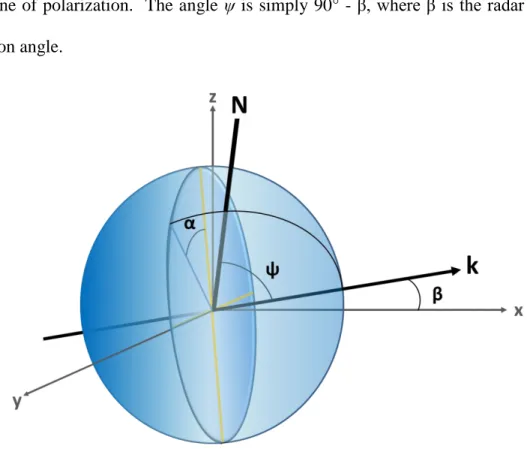
backscattered signal. If we define k = ̂ as the direction of the incident wave propagation, then the backscattered signal direction is ̂ . In general, hydrometeors can be canted with respect to the plane of polarization. The geometry of such scattering is shown in Figure 1.1. The hydrometeor canting can be described by two angles: (1) canting of the particle within the plane of polarization, α, and (2) the canting of the particle out of the plane of polarization, ψ. The angle α is taken between the projections of the true vertical and the axis of symmetry of the hydrometeor N onto the plane of polarization. The angle ψ is simply 90° - β, where β is the radar antenna elevation angle.

Fig. 1.1: Geometry of scattering. The Cartesian axes x, y, and z are shown in gray (z represents the true vertical). The plane with orthogonal yellow lines represents the plane of polarization, which is embedded within a spheroidal hydrometeor with symmetry axis N. The direction of wave propagation is k, which is at elevation angle β. The particle orientation is given by two angles: α, which is its canting angle within the plane of polarization (with respect to vertical polarization), and ψ, which is the angle between the propagation direction and symmetry axis of the particle (in other words, 90° - ψ represents the canting angle out of the plane of polarization).

(34)

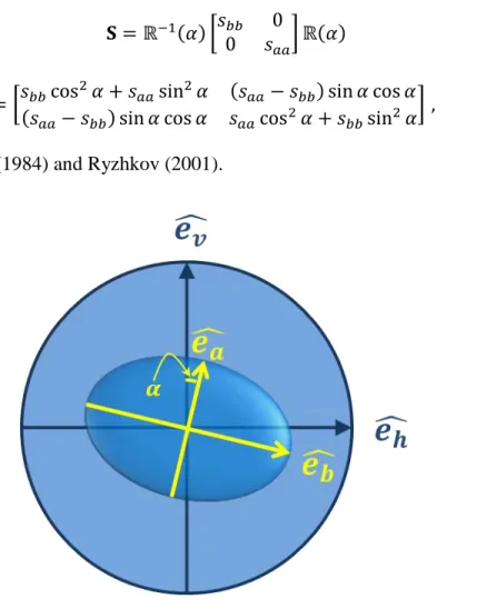
Simple geometric considerations (Fig. 1.2) allow us to account for canting within the plane of polarization (i.e., α ≠ 0°). The incident radiation at both polarizations will each have components along (and thus excite) the dipoles aligned with the particle’s major and minor axes (b and a). Thus, the incident radiation at H and V polarizations can be expressed as

̂ ̂ ̂ ̂ ̂ ̂ ̂ ̂ ̂ ̂

where we have defined the unit directional vectors ̂ and ̂ as the direction of H and V polarizations, and ̂ and ̂ as along the particle’s major and minor axes (see Fig. 1.2). Note that the relation between the principal polarization axes and the particle’s major and minor axes is given by a simple rotation matrix, :

[̂_{̂] [} ] [ ̂ ̂ ] [ ̂ ̂ ]

The scattered radiation is proportional to the component of incident radiation that illuminates each dipole, as well as the complex scattering function2 of each dipole:

[ ] [ ] [ ]

However, because the radar receives signals at H and V polarization, we must rotate the reference frame back to (H,V) using the inverse of the rotation matrix, :

[ ] _[ ] [ ]

It is clear from inspection of eqns. (1.3) and (1.7) that the scattering matrix S can be written as

(35)

_[

]

[

]

following Holt (1984) and Ryzhkov (2001).

Figure 1.2: View of the polarization plane (blue circle) illuminating a raindrop canted within the plane of polarization at angle α. The direction of wave propagation k is into the page. The raindrop’s major and minor axes (yellow arrows) are in the ̂ and ̂ directions, respectively.

Equation 1.8 is a special case of when the particle’s symmetry axis N is aligned within the plane of polarization (i.e., ψ = 0°). In general, however, ψ ≠ 0°, in which case the complex scattering functions sbb and saa are functions of ψ. Holt and Shepherd

(1979) derive these functions in the Rayleigh approximation in what is known as the “backscatter rule”:

where fa (fb) is the complex scattering function of the particle if the electric field vector

(36)

approximation is valid in raindrops for radar wavelengths > 0.9 cm and for elevation angles < 10°. At S band, this “backscatter rule” is valid for most hydrometeors except large hail. Thus, substituting eqn. (1.9) into eqn. (1.8), we obtain

[

…

]

After using several trig identities, the expression simplifies to

[

]

2. Calculating the Complex Scattering Functions

The complex scattering functions fa,b in eqn. (1.11) characterize the

electromagnetic response of particles illuminated by incident radiation. In general, fa,b

are functions of the wavelength of the incident radiation, and the irradiated particle’s properties, including size, shape, temperature, and composition. The particle’s composition affects its complex dielectric factor ε = ε’ - j ε’’, which is a measure of a material’s electromagnetic response when irradiated. The complex scattering functions can be calculated using approximate analytical formulas (e.g., Rayleigh 1871; see also Doviak and Zrnić 1993), or more rigorous numerical techniques such as the T-Matrix method (e.g., Waterman 1969; Vivekanandan et al. 1991; Mishchenko 2000) or the discrete dipole approximation (see reviews by Draine 1988; Draine and Flatau 1994). The range of validity for these methods depends on the wavelength of the incident radiation , as well as the characteristic size and composition of the particle being

(37)

radiated. For hydrometeors treated as spheroids, it is convenient to use the resonance parameter

√| |

where D is the equivalent spherical diameter of the spheroid, and ε is the complex dielectric factor. The resonance parameter is unity at the peak of the first resonance; depending on the application and desired accuracy, thresholds of 0.6 – 0.8 are used to determine the limits of the Rayleigh approximation (e.g., Ryzhkov et al. 2011).

a. Rayleigh Approximation

Under the Rayleigh approximation to the Mie (1908) solution of scattering by a sphere, the complex scattering functions are given by

where the polarizability factors of the particle along its minor and major axes are

Note in eqn. (1.13) that the forward and backward scattering functions (superscript 0 and , respectively) are identical in the Rayleigh approximation. In eqn. (1.14), we have defined the shape parameters , which are functions only of the particle axis ratio, ⁄ . For spherical particles, , and the shape parameters

⁄ . For oblate particles, b > a, and

[

√

√ ]

(38)

[_√ (

√

√ ) ]

The shape factors are shown in Figure 1.3. If we assume the particle is spherical with the same volume as the oblate or prolate spheroid, eqn. (1.13) can be simplified to

In the case of mixed-phase particles (e.g., melting hail, freezing raindrops), it is convenient to use the two-layer spheroid model (e.g., Bohren and Huffman 1983). If the volume fraction of the inner spheroid is 1, the complex scattering functions of the two-layer particle are given by

[ ]

[ ][ ]

In eqn. (1.18), the complex dielectric factors 1 and 2 correspond to the inner and outer spheroid, respectively (Fig. 1.4).

The Rayleigh formulas work well for computing radar variables based on the “real” parts of the complex scattering functions, for values of resonance parameter << 1.0. However, they should not be used to calculate variables related to the “imaginary” parts of the scattering functions for any value of , as the values provided are inaccurate.

(39)

Fig. 1.3: Shape factors and for oblate (top panel) and prolate (bottom panel) spheroids.

Fig. 1.4: Geometry of the two-layer spheroid, with an inner spheroid of dielectric constant 1

and outer dielectric 2. The silhouette of the inner spheroid is shown by the gray dashed curve.

3. The Covariance Matrix

Radar meteorologists process the received raw complex voltages to obtain the second-order moments, because the expected value or mean (first order moment) composite voltage over an ensemble of hydrometeors sums to zero owing to the random

0 0.2 0.4 0.6 0.8 1 0 0.2 0.4 0.6 0.8 1 a / b L a , L b Oblate spheroids L_a L_b 0 0.2 0.4 0.6 0.8 1 0 0.2 0.4 0.6 0.8 1 b / a L a , L b Prolate spheroids L_a L_b

(40)

phase of the individual contributions (Zrnić 1991). A fully polarimetric radar can measure all quantities in the “covariance matrix” C, defined in the linear (HV) basis as (Zrnić 1991) [ 〈 〉 〈 〉 〈 〉 〈 〉 〈 〉 〈 〉 〈 〉 〈 〉 〈 〉 ] [ 〈| | 〉 〈 〉 〈 〉 〈 〉 〈| | 〉 〈 〉 〈 〉 〈 〉 〈| | 〉 ]

In eqn. (1.19), angle brackets denote ensemble averaging, and the asterisk represents the complex conjugate. Note that the covariance matrix in (1.19) has been reduced from its more general 4x4 form by assuming reciprocity ( The diagonal elements of (1.19) are magnitudes only and represent the received polar H, cross-polar, and co-polar V powers. These diagonal elements contain no phase information, whereas the off-diagonal elements are complex and thus contain both power and phase information. This is evident by examining one of these elements (e.g., C13) in expanded form:

〈 〉 〈| | [ ]〉

The phase angles ij = i – j represent the phase lag or lead between the backscattered

radiation (i polarization) and the incident radiation (j polarization) at the location of the scatterer. In other words, in the absence of propagation effects, the co-polar phase angle ii represents the phase shift imparted on the i-polarization radiation upon

backscatter. Thus, the argument of the element C13 is the co-polar differential phase shift upon backscatter, herein denoted as

 .

Because of the symmetry in (1.19), the element C31 is simply -; thus, it is considered non-unique. The remaining off-diagonal elements that provide unique phase

(41)

〈 〉 〈| | [ ]〉 〈| | 〉 〈 〉 〈| | [ ]〉 〈| | 〉.

Note that we have defined as the so-called depolarization phase shifts (Ryzhkov 2001). To summarize the phase information available in the covariance matrix, we define the “covariance phase matrix”:

[

]

4. Polarimetric Radar Variables from the Covariance Matrix

The elements of the covariance matrix are used to infer physical properties of the hydrometeors within the radar sampling volume. The co-polar power at H polarization (C11 in eqn. 1.19) is related to the radar reflectivity factor at horizontal polarization:

| | 〈| | 〉

In eqn. (1.21), the dielectric factor | ⁄ | is written as | | Note that the coefficient comes from a normalization such that for small scatterers, Zh is identical to the Rayleigh reflectivity (based on eqn. 1.13). Similarly, the co-polar power at V polarization (C33) is related to the radar reflectivity factor at vertical polarization:

| | 〈| | 〉

The ratio of these co-polar powers is the differential reflectivity factor: