Violent scene detection using a super descriptor tensor decomposition

(1)

University of Wollongong

Research Online

Faculty of Engineering and Information

Sciences - Papers: Part A

Faculty of Engineering and Information

Sciences

1-1-2015

Violent scene detection using a super descriptor tensor decomposition

Muhammad Rizwan KHOKHER

University of Wollongong, [email protected]

Abdesselam Bouzerdoum

Son Lam Phung

Follow this and additional works at: https://ro.uow.edu.au/eispapers

Part of the Engineering Commons, and the Science and Technology Studies Commons

Recommended Citation

KHOKHER, Muhammad Rizwan; Bouzerdoum, Abdesselam; and Phung, Son Lam, "Violent scene detection using a super descriptor tensor decomposition" (2015). Faculty of Engineering and Information Sciences - Papers: Part A. 5435.

https://ro.uow.edu.au/eispapers/5435

Research Online is the open access institutional repository for the University of Wollongong. For further information contact the UOW Library: [email protected]

(2)

Violent scene detection using a super descriptor tensor decomposition

Abstract

This article presents a new method for violent scene detection using super descriptor tensor

decomposition. Multi-modal local features comprising auditory and visual features are extracted from Mel-frequency cepstral coefficients (including first and second order derivatives) and refined dense trajectories. There is usually a large number of dense trajectories extracted from a video sequence; some of these trajectories are unnecessary and can affect the accuracy. We propose to refine the dense trajectories by selecting only discriminative trajectories in the region of interest. Visual descriptors consisting of oriented gradient and motion boundary histograms are computed along the refined dense trajectories. In traditional bag-of-visual-words techniques, the feature descriptors are concatenated to form a single large feature vector for classification. This destroys the spatio-Temporal interactions among features extracted from multi-modal data. To address this problem, a super descriptor tensor

decomposition is proposed. The extracted feature descriptors are first encoded using super descriptor vector method. Then the encoded features are arranged as tensors so as to retain the spatio-Temporal structure of the features. To obtain a compact set of features for classification, the TUCKER-3

decomposition is applied to the super descriptor tensors, followed by feature selection using Fisher feature ranking. The obtained features are fed to a support vector machine classifier. Experimental evaluation is performed on violence detection benchmark dataset, MediaEval VSD2014. The proposed method outperforms most of the state-of-The-Art methods, achieving MAP2014 scores of 60.2% and 67.8% on two subsets of the dataset.

Keywords

super, descriptor, tensor, scene, decomposition, detection, violent

Disciplines

Engineering | Science and Technology Studies

Publication Details

M. Khokher, A. Bouzerdoum & S. Lam. Phung, "Violent scene detection using a super descriptor tensor decomposition," in Digital Image Computing: Techniques and Applications (DICTA), 2015 International Conference on, 2015, pp. 1-8.

(3)

Violent Scene Detection using a Super Descriptor

Tensor Decomposition

Muhammad Rizwan Khokher, Abdesselam Bouzerdoum, Son Lam Phung

School of Electrical, Computer and Telecommunication Engineering University of Wollongong, NSW, 2522, Australia

[email protected], [email protected], [email protected]

Abstract—This article presents a new method for violent scene detection using super descriptor tensor decomposition. Multi-modal local features comprising auditory and visual features are extracted from Mel-frequency cepstral coefficients (including first and second order derivatives) and refined dense trajectories. There is usually a large number of dense trajectories extracted from a video sequence; some of these trajectories are unnecessary and can affect the accuracy. We propose to refine the dense trajectories by selecting only discriminative trajectories in the region of interest. Visual descriptors consisting of oriented gradient and motion boundary histograms are computed along the refined dense trajectories. In traditional bag-of-visual-words techniques, the feature descriptors are concatenated to form a single large feature vector for classification. This destroys the spatio-temporal interactions among features extracted from multi-modal data. To address this problem, a super descriptor tensor decomposition is proposed. The extracted feature descriptors are first encoded using super descriptor vector method. Then the encoded features are arranged as tensors so as to retain the spatio-temporal structure of the features. To obtain a compact set of features for classification, the TUCKER-3 decomposition is applied to the super descriptor tensors, followed by feature selection using Fisher feature ranking. The obtained features are fed to a support vector machine classifier. Experimental evaluation is performed on violence detection benchmark dataset, MediaEval VSD2014. The proposed method outperforms most of the state-of-the-art methods, achieving MAP2014 scores of 60.2% and 67.8% on two subsets of the dataset.

Keywords—Violent scene detection; refined dense trajectories; super descriptor vector; tensor decomposition; support vector machines

I. INTRODUCTION

We live in an era where human interaction with moving images has become an affective tool for shaping one’s personality and character. The video material including television programs, movies and internet videos has increased rapidly in the last few decades. The ease of accessibility to a huge video enterprise via video-on-demand has raised the necessity of filtering the video content. The applications range from surveillance to parental control. For example, it is very important for the parents to filter inappropriate content (e.g., violence) for their children. Violence can affect a child’s personality in a harmful way. Although there are different movie ratings available, the interpretation of the word violence varies from one

individual to another. The material uploaded online usually does not have any content description in terms of violence. With this in view, there is a need to develop some methods to recognize and analyze the video content, in order to assist parents decide for themselves whether a video is appropriate for their children or not.

The task of violent scene detection (VSD) has been studied before, especially in the video surveillance domain. In the case of movies, the VSD task is significantly different where so many audio and visual effects are involved due to high editing. In this article, we focus on VSD in movies and user generated videos uploaded on internet (e.g., YouTube). The task becomes complex due to the subjective and ambiguous definition of violence. This causes researchers difficulty in terms of working on a common ground [1]. Some of the violence interpretations include violent actions by humans where there is blood [2], scenes containing gunshots, fights and explosions [3], person to person harmful acts like threatening and physical harm [4], and fighting scenes regardless of number of individuals involved and context [5, 6]. These different interpretations lead to different techniques for VSD, which makes it difficult to conduct a comparative study. Furthermore, the presence of multiple modalities and unknown duration of events complicate the problem further.

The different approaches can be categorized in terms of feature types extracted for classification (i.e., audio, visual and textual). For example in [7, 8], the authors used single modality (i.e, audio events) and extracted different audio features including zero crossing, energy entropy and some other audio features. Many researchers, on the other hand, have been interested in combining both auditory and visual modalities. The combined use of audio (e.g., chroma, spectrogram and Mel-Frequency Cepstral Coefficients (MFCC)) and visual features (e.g., motion based variance, motion of people and average motion) produced some good results [4]. In [9], the authors performed a modified probabilistic Latent Semantic Analysis (pLSA) based violence detection from audio cues and visual information by exploiting different concepts (including explosion, motion, blood and flame etc.). Many other methods have been proposed that merge the two modalities of audio and visual information for VSD, e.g., [10–13]. Other than audio-visual features, some authors also exploited the use of textual

(4)

information [14, 15].

Recently, MediaEval has been providing a benchmark for VSD task in movies since year 2011 [16]. The Affect Task of MediaEval has provided a common ground for researchers to work on this problem and compare their algorithms in an efficient way. A publicly available dataset provides a detailed annotation ground truth of multiple audio and visual concepts concerning violence [17]. In MediaEval 2014, many teams participated for the VSD task [17]. In [18], the authors used Deep Neural Networks (DNN) along with Support Vector Machines (SVM) and extracted different audio-visual features (i.e., MFCC, dense trajectories [19], spatio-temporal interest points (STIP)). This method performed best of all on one of the two VSD sub-tasks (i.e., violence detection in Hollywood movies). In [20], a set of mid-level concepts was predicted from many low level audio and visual features and then the features and concept predictions were fused to detect the violent scenes. This approach outperformed the other methods on the second VSD sub-task (i.e., violence detection in user generated videos from YouTube). The most common features used by most of the participating teams were MFCC (audio) and dense trajectories (visual+temporal) [17].

The adaptation of dense trajectories method is motivated by the fact that it is based on derivatives of optical flow [19, 21]. The motion boundary histogram (MBH) descriptor computed along dense trajectories helps suppress the irrelevant motion patterns in a simple and efficient way [22]. Even though the dense trajectory method performs very well in comparison with others, it still faces challenges due to fast view point changes along with camera motion and other visual effects present in movies. One of the reason is that there are too many trajectories computed, which increases the complexity. We propose to refine the dense trajectories by selecting discriminative trajectories present in the region of interest (ROI). This can further suppress the effects of camera motion and other noise factors.

The bag-of-visual-words (BoVW) model has been used widely for global feature representation. However, more recently super vector based methods, such as super vector coding (SVC) [23], Fisher vector (FV) [24] and vector of locally aggregated descriptors (VLAD) [25], have been proposed with promising results. These methods aggregate high order statistics and yield very high dimensional representations. In BoVW pipeline, the code vectors are obtained after super vector based coding for individual local feature descriptors. These code vectors are usually concatenated to get a single vector for the whole video segment. This does not retain the structure of interactions between the local feature descriptors. Rather than forming a one dimensional vector, it is more efficient to deal with the data in multidimensional arrays (i.e., tensors). Tensors provide a natural way to represent the multi-modal data (i.e, audio, visual modalities). By arranging the data after some super vector based coding, multidimensional tensors can be formed, and some tensor decomposition (e.g., TUCKER and

PARAFAC) can be applied. The tensor decomposition is important for high detection accuracy because it discards the noise and retains the information that is most discriminative, while achieving dimensionality reduction.

We propose a new method for VSD based on a tensor representation of auditory and visual features. The local features are extracted through MFCC from audio and refined dense trajectories from video signals. The local feature descriptors are encoded through a super vector based method using Gaussian mixture model (GMM) and sparse coding. The data is arranged as tensors, and the TUCKER-3 decomposition [26] is performed to reduce the dimension and filter out noisy features. The optimal number of features are selected based on the Fisher score for classification using SVM.

The remainder of the paper is organized as follows. Local feature extraction using MFCC and proposed refined dense trajectories method is explained in Section II. In Section III, the proposed super descriptor tensor decomposition (SDTD) model is presented. The experimental methods, results and analysis are given in Section IV. Section V concludes the paper.

II. LOCALFEATUREEXTRACTION

The proposed VSD approach exploits both audio and visual modalities to benefit from a multi-modal structure of the movies. The MFCC [27] features along with their first and second order derivatives are used for the audio modality. For the visual modality, we adapt the dense trajectories proposed by Wang et al. [21] to extract the local motion features from the video segments [21]. However, the visual features are extracted from refined dense trajectories, which are presented in Subsection II.B.

A. Mel-Frequency Cepstral Coefficients

Mel-frequency cepstral coefficients are commonly used in automatic speech recognition [27]. We briefly describe the MFCC method here. Firstly, the audio signal is segmented into short frames with some overlap. The reason for keeping the frames short is that the audio signal is assumed to be stationary over short durations. A power spectrum of each frame is calculated using the periodogram. Then a mel-filterbank of triangular filters is applied to the power spectra, and energy in each filter is summed up. To match the features closely to human hearing, the logarithms of all the filterbank energies are computed. As the filterbanks are usually overlapping in the frequency domain, a discrete cosine transform (DCT) is applied to the log filterbank energies. In the end, a set of lower DCT coefficients is taken which represents the MFCCs. In order to exploit the complete discriminative ability of MFCC, first and second order derivatives of MFCC features are also used.

B. Refined Dense Trajectories

The visual features are extracted based on dense trajectories method proposed by Wang et al.[21]. The dense

(5)

Fig. 1: Illustration of the refined dense trajectories method adapted from [21]. (a) A grid is used to densely sample the features points for each spatial scale. (b) The sample points are refined by incorporating only those points that are present in the ROI. (c) A median filter and dense optical flow field is used to track the points in each spatial scale. (d) Descriptors like HOG and MBH are computed along the dense trajectories within a volume of N×N×Lwhich is subdivided intonσ×nσ×nT.

trajectories are computed using multiple spatial scales. A grid is used to densely sample the sample points which are separately tracked in each spatial scale. The problem using the dense trajectories is that usually there are too many sample points that are required to be tracked. This results in excessive trajectories that add noise and reduce the accuracy. In order to obtain discriminative trajectories, we propose refined dense trajectories to incorporate only those points that are present in the ROI. The ROI represents the region where motion is observed. To find the ROI, a dense optical flow field is calculated. Here, the algorithm by Farneback [28] is used to extract dense optical flow as it embeds a translational motion model between two consecutive frames. Irregular and fast motion patterns can easily be tracked because of the smoothness constraints of the dense optical flow field. Motion detection is performed by calculating the magnitude of gradient of the optical flow, yielding a gray level image that provides the information about motion areas. Once the ROI is calculated, the gray level motion image is converted to a binary image by thresholding. For this purpose, minimum error thresholding by Kittler et al. is used [29]. The gray level histogram is considered as an estimate of the probability density function of the mixture population of the gray levels of the foreground and background pixels. The foreground and background class conditional probability density functions are assumed to be Gaussian. Initially, an arbitrary threshold τ is used to divide the histogram. Then an optimum threshold τopt is calculated

by minimizing the following expression:

(1)

τopt= arg min

τ [P(τ) logσf(τ) + (1−P(τ)) logσb(τ)

−P(τ) logP(τ)−(1−P(τ)) log(1−P(τ))],

where σf(τ) and σb(τ) are the foreground and background

variances respectively for threshold τ, andP(τ) representsa

priori probability of gray levels below the threshold τ. For further details of minimum error thresholding, see [29]. After performing the thresholding operation, a mask is obtained, which is then applied to the dense feature points to delete all invalid points from the ROI. Fig. 1(a) shows a frame of a sports fighting scene from VSD2014 dataset [17]. One can see the extra red points representing the end points of the trajectories all over the static textured regions of the scene. The trajectories computed through the refined dense trajectories method are shown in Fig. 1(b), where the trajectories are refined to get the discriminative motion information of the scene.

In order to track the sample points to form trajectories, the same procedure is used as in [21]. Here we describe the procedure briefly. First, the refined sample points are tracked in the succeeding frames by applying a median filter on the dense optical flow field. A trajectory is formed by concatenating tracked points in subsequent frames. The trajectories are tracked up to L frames only because they have a tendency to drift from their point of initialization, as shown in Fig. 1(c). Descriptors like HOG and MBH are computed along the trajectories within a space-time volume which leverages the motion information. The space-time volume with dimensions N ×N×L is further divided into smaller grids of size nσ × nσ × nT. This embeds the

structure information as shown in Fig. 1(d). The HOG descriptor concentrates on the static appearance information, while MBH extracts the dynamic information. The MBH descriptor computes the spatial derivatives along the vertical and horizontal components of the optical flow field, which encodes the relative motion between pixels [22]. The orientations are quantized into β bins for HOG and each component of MBH (i.e., MBHx and MBHy). Finally, L2 norm is used for the normalization of the descriptors.

(6)

III. SUPERDESCRIPTORTENSORDECOMPOSITION

Here, we propose the super descriptor tensor decomposition model to obtain the discriminative features for classification. Firstly, the audio and visual features are encoded through super descriptor vector coding. The encoded features are then represented as tensors, discriminative features are obtained through a tensor decomposition and feature selection.

A. Super Descriptor Vector

The super descriptor vector (SDV) coding [30] is used here to encode the features. For each video segmentV, a set of descriptors X = {xi, ...,xn}, xi ∈ Rm, is obtained for

each feature type (i.e., MFCC, HOG, MBHx and MBHy). Let D={d1, ...,dK} be a dictionary with K visual words,

dk ∈ Rm. The descriptors xi are modeled using GMM as

follows: p(xi) = K ∑ k=1 wkp(xi|k), (2)

where wk is the mixture weight of the kth component

density p(xi|k). The mixture weightwk corresponds to prior

probability that xi was generated by component k. The kth

component density is a normal probability density function with mean vectorµµµ_k and covariance matrixΣk,

p(xi|k) =N(xi;µµµk,Σk). (3)

The probability density function in Eq. (2) models the generation process of xi. The gradient of the log-likelihood

with respect to mean expresses the contribution of mean as follows: ∂ lnp(xi) ∂µµµ_k =p k iΣ− 1 k (xi−µµµk), (4) wherepk

i denotes the posterior p(k|xi).

Here sparse coding is used to learn the visual dictionary because it is computationally less expensive than the Expectation Maximization (EM) [31]. Sparse coding approximates xi by using a linear combination of a limited

number of visual words. The ℓ1 penalty yields a sparse solution for the following sparse coding problem,

(5) min D,ααα 1 n n ∑ i=1 1 2||xi−Dαααi|| 2 2+λ||αααi||1, subject to dTkdk ≤1,

where λ is the sparsity-inducing regularization that controls the number of non-zero sparse coding coefficients inαααi. For

further details on sparse coding based dictionary learning, see [31].

After learning the dictionary D={d1, ...,dK}and finding

the sparse coding coefficients αααi for every xi, a few

approximations are made to simplify Eq. (4). First, sparse coding coefficients are used to estimate the posterior, i.e.,

pk

i =αki, where αki is the coefficient of the ith descriptor xi

to the kth visual word dk. Second, the mean is represented

by the visual word in sparse coding, i.e.,µµµ_k =dk. Third, the

covariance is assumed to be isotropic, i.e., Σk =σ2I. After

these three approximations the RHS in Eq. (4) becomes

αk

i(xi−dk). Then for each visual word, average pooling is

used to aggregate the weighted difference vectors: uk= 1 n n ∑ i=1 αk_i(xi−dk). (6)

In the BoVW models, the vectors uk, k = 1, ..., K are

simply concatenated to get a large single vector for classification. This does not retain the structure of interactions between the features. To address this problem, we propose to arrange the coded vectors after SDV encoding in the form of tensors. For this purpose, the vectors uk, are

arranged into a K×m matrix. For l different feature types (i.e., MFCC, HOG, MBHx and MBHy), the resultantK×m

matrices are arranged as rank 3 tensor X ∈ R K×m×l_{, for}

each video segment.

B. Tensor Decomposition

The tensor X contains a large number of features. To discard noisy features and get the most discriminative and compact set of features for classification, tensor decomposition is applied. Assume we have a rank 3 tensor X(i)∈RK×m×l,i= 1,2, ..., Qfor each video segment. The tensor decomposition of X(i) to get three basis factors

A(1) _∈_RK×J1_{, A}(2)∈Rm×J2 _and_A(3)∈Rl×J3_{, is given} as

X(i)≈G(i)×1A(1)×2A(2)×3A(3), (7) G(i) ∈ R J1×J2×J3 _{is the feature core tensor of the data} tensor X(i). There are in total J1×J2×J3 number of features. ×p, p = 1,2,3, is the p-mode product of a tensor

by a matrix. For example, let G(i) = {gj1,j2,j3} and

A(1)_{= [}_a k,j1], (8) (G(i)×1A(1))k,j2,j3 = ∑ j1 gj1,j2,j3∗ak,j1.

The basis factor A(p) _{can be obtained by minimizing the} following cost function,

arg min {A(1)_,A(2)_,A(3)_} Q ∑ i=1 ∥X(i)−G(i)×1A(1)×2A(2)×3A(3)∥2F, (9) where∥·∥2_F is the Frobenius norm.

The Q simultaneous standard decompositions of rank 3 tensors X(i) in Eq. (7) are equivalent to the following tensor decomposition:

X≈G×1A(1)×2A(2)×3A(3), (10) where the tensorsX∈RK×m×l×Q _and_G_∈_RJ1×J2×J3×Q are rank 4 tensors obtained by concatenating all the tensors X(i) and G(i) along the mode-4. This unique decomposition

(7)

Fig. 2: Illustration of the proposed SDTD method. First, the individual tensors obtained after the SDV coding are concatenated to get final tensorsXandXtfor training and test dataset respectively. The training tensorXis decomposed through TUCKER-3 tensor decomposition using orthogonal interactions. Training features are obtained from the core tensorGafter decomposition. The orthogonal basis factorsU are used to get the test features fromGt=Xt× {UT_}_{. The feature selection for training and}

test features is performed on basis of their Fisher score. In the end, linear SVM is used to classify the video segments.

model is called TUCKER-3 tensor decomposition. For the detailed mathematical model, see [26].

In order to obtain meaningful and unique TUCKER-3 representation, orthogonality constraints are applied, such a model is called higher order singular value decomposition (HOSVD) or higher order orthogonal interactions (HOOI) [32, 33]. Orthogonal interactive basis are estimated as factors

A(p) =U(p) of the TUCKER-3 decomposition of the tensor X. First, the factors U(p) are randomly initialized so that the core tensor Gcan be obtained [32, 33],

G=X×1U(1)T ×2U(2) T ×3U(3) T. (11) Then the following cost function is maximized to find the factorsU(p)_,

J(U(p)) =∥X×1U(1)T ×2U(2) T ×3U(3) T∥2F, (12)

where only U(p) are unknown. If we fix U(p), the tensor X can be projected onto the subspace defined as

(13) W(−p)=X×1U(1) T×2U(2)T ×3U(3)T

=X×₋(p,4){UT}. The factors U(p) _{can be estimated as} _J

p which are leading

left vectors of the mode-pmatricized version ofW₍(_p−₎p). This leads to HOOI algorithm [33]. Once the basis factorsU(p)are obtained, the test feature core tensor Gt for a test tensor Xt can be obtained as Gt=Xt× {UT} as shown in Fig. 2.

C. Feature Selection and Classification

It is likely that some discriminative features will be lost if the size of the core tensor is set too small during the tensor decomposition. But avoiding feature loss can cause the core tensor to be large for efficient classification. To solve this

problem, the salient features for classification are selected using Fisher ranking [26]. The Fisher score of theqth feature is defined as, φ(q) = ∑C j=1Qj(¯g (j) q −¯¯gq)2 ∑Q i=1(g (i) q −¯g (ji) q )2 , (14)

whereg(qi)is theqth feature (entry)(q= 1,2, ..., J1×J2×J3) of the vectorized version of feature core tensor G(i), ji =

1,2, ..., C is the class of the training sample X(i) andQj is

the number of training samples in class j. The mean sample

¯

gq(j) for the jth class of the qth feature and the total mean

feature ¯¯gq are defined as,

¯ gq = 1 Qj ∑ i_∈j g_q(i), ¯¯gq= 1 Q Q ∑ i=1 g_q(i). (15) The features are sorted in a descending order of their Fisher score. The top features are selected for the classification using a linear SVM. The optimal number of features that can achieve the best performance is selected through experimentation on a the validation dataset.

IV. RESULTS ANDANALYSIS A. Dataset and Evaluation Criterion

We test the SDTD method on publicly available benchmark MediaEval VSD dataset [17]. The VSD2014 dataset contains three subsets: Development, Test and

Generalization subsets. The Development and Test subsets consist of Hollywood movies and the Generalization subset contains video clips from YouTube. There are twenty four movies in the Development, seven movies in the Test and eighty six clips in the Generalization subsets, with average

(8)

Fig. 4: MAP2014 score vs. number of features for (a) Hollywood movies and (b) YouTube clips. Top features are selected according to their Fisher scores.

Fig. 3: Sample video frames from the MediaEval VSD2014 dataset [17].

violence rate of 12.35%, 17.18% and 31.69%, respectively. Frame level binary annotations are provided for all the scenes. The violent scenes are identified by their start and end frames. Fig. 3 shows some violent scenes (explosion, fights, gun-shot, screaming and war violence etc.) from the VSD2014 dataset.

In order to become consistent with the participating teams in VSD2014 task, we perform the same violence detection task and use the same evaluation measure. The VSD Affect Task [17] at MediaEval 2014 aimed to auto-detect the violent video segments in movies by indicating their start and end frames. With this information it is easy to make a summarized video containing violent scenes for parental guidance. For evaluation, a modified version of the mean

average precision (MAP), dubbed MAP2014, was used [17]. The MAP2014 measure considers as a hit only predicted segments that overlap by more than 50% with their corresponding ground truth segments. If there are multiple hits on the same ground truth, only one true positive is counted and the rest are ignored.

B. Implementation

For MFCC audio features, the frame size is set to 40ms with 20ms overlap, to make alignment with dataset videos encoded with 25 fps. From each frame, 96 dimensional vector is computed comprising MFCCs and their first and second order derivatives using the MIRtoolbox [34]. For the visual features from refined dense trajectories, 8 spatial scales are used. The size of the median filter kernel is3×3. The length of the trajectories is set to L = 15 frames. The parameter values for volumeN×N×Land spatio-temporal gridnσ×

nσ×nτ are set toN = 32,nσ= 2andnτ = 3. For an8bin

quantization of orientations, the final dimension of the HOG, MBHx and MBHy descriptors is96each.

For the SDV coding, the number of visual words is set to

500. The code vectors are arranged into a 500×96 matrix. For the four feature types (i.e., MFCC, HOG, MBHx and MBHy), a 3D tensor is obtained of size 500×96×4 for each video segment. These 3D tensors are concatenated to yield a training tensor for the video segments from the training subset. The TUCKER-3 tensor decomposition is implemented using “NFEA” toolbox [35].

Finally for the classification, a linear SVM is used for the training and testing. The parameters for the linear SVM are optimized through a 5-fold cross validation on the training subset (i.e., Development). The LIBLINEAR toolbox [36] is used to implement the linear SVM. The videos in the test subsets (i.e.,Test andGeneralization) are subdivided into 75 frames clips. For the desired segment level prediction output,

(9)

the continuous clips are merged to get a single video segment if they are all classified as violent or non-violent.

C. Violent Scene Detection

In first experiment, we analyze the effect of the number of features used for classification. After the tensor decomposition, the features are sorted in a descending order according of their Fisher score, and the top features are selected as inputs to the classifier. Fig. 4 illustrates the MAP2014 scores as a function of the number of selected features. From this figure, we can see that the top 600

hundred features achieve MAP2014 score of more than 50%. The highest MAP2014 scores of 60.2% (Fig. 4(a)) and

67.8% (Fig. 4(b)) are achieved by using 4400 and 3200

features on the Test andGeneralization subsets, respectively. These are the optimal number of features that achieve the best performance. For both subsets, the number of features for a video segment are significantly reduced, from

500×96×4 = 192000 to4400and3200.

In the second experiment, we compare the SDTD method with some BoVW methods. Firstly, a dictionary is created with500 visual words usingK-means [37]. The LLC coding [38] encodes the audio-visual local features. These encoded features are then pooled and normalized using max pooling and power plus L2 normalization [39]. The resultant global features are then fed to a linear SVM for classification. By applying this BoVW model, MAP2014 scores of 54.1%and

59.6% are achieved on Test and Generalization subsets (Table I, LLC+SVM). Secondly, the SDV encoded features are directly fed to a linear SVM by simply concatenating the code vectors. There is no tensor decomposition performed on the features. This model is another example of BoVW model, where raw features from descriptors are encoded and pooled to get a global representation for classification. Here, the MAP2014 scores of58% and65.4% are achieved on the two subsets (SDV+SVM in Table I). It’s clear from the results in Table I that the SDV outperforms the LLC coding in the BoVW pipeline. Thirdly, the SDTD method performs better than the above two BoVW models; it achieves scores of 60.2% and 67.8% on the two subsets. This is because representing the features in a tensor form retains the interactions between the features that is destroyed if they are concatenated directly. There are too many features that add noise and affect the accuracy. In order to obtain the salient features, tensor decomposition along with Fisher ranking provides a better way for dimensionality reduction without compromising on the accuracy.

TABLE I: MAP2014 scores of the SDTD method and BoVW methods on the Test(Hollywood) and Generalization

(YouTube) subsets.

LLC+SVM SDV+SVM SDTD+SVM

Test(Hollywood) 54.1% 58.0% 60.2%

Generalization(YouTube) 59.6% 65.4% 67.8%

In the third experiment, we compare the SDTD approach

with several methods presented for the VSD task at MediaEval 2014 [17]. The participating teams include FUDAN [18], FAR [20], NII-UIT [40], MIC-TJU [41],

RECOD [15], VIVOLAB [42], TUB-IRML [43] and

MTMDCC [44]. The MAP2014 scores for the SDTD and previous methods on Test (Hollywood) and Generalization

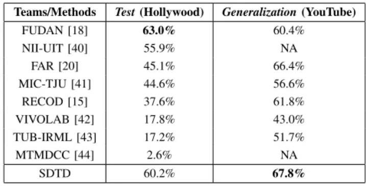
(YouTube) subsets are given in Table II. For the Hollywood movies, our SDTD method achieves a score of 60.2% and outperforms every other method except for FUDAN that has a score of 63%. One of the reasons of reduced performance can be a great amount of camera motion and variation in view point in the movies. Although the MBH descriptor along with the refined dense trajectories helps suppress the camera motion, there is still enough room for improvement. The SDTD method outperforms FUDAN and all other methods onGeneralization(YouTube) subset. The MAP2014 score achieved by the proposed method is 1.4%than that of the best performing team FAR.

TABLE II: MAP2014 scores of the SDTD method and the VSD2014 participating teams on the Test (Hollywood) and

Generalization (YouTube) subsets.

Teams/Methods Test(Hollywood) Generalization(YouTube)

FUDAN [18] 63.0% 60.4% NII-UIT [40] 55.9% NA FAR [20] 45.1% 66.4% MIC-TJU [41] 44.6% 56.6% RECOD [15] 37.6% 61.8% VIVOLAB [42] 17.8% 43.0% TUB-IRML [43] 17.2% 51.7% MTMDCC [44] 2.6% NA SDTD 60.2% 67.8% V. CONCLUSION

This paper presents a new method for violent scene detection using a super descriptor tensor decomposition. The audio and visual local features are extracted from the video segments via MFCC, HOG, MBHx and MBHy descriptors. The proposed refined dense trajectories method excludes the extra trajectories by incorporating only those that are present in the region of interest. The feature descriptors are encoded through super descriptor vector method. The encoded features are represented as tensors in order to retain the interactions between the features. The number of features are significantly reduced through TUCKER-3 tensor decomposition and Fisher score based selection. This provides a way to extract the discriminative features required for the classification, in addition to dimensionality reduction. In the end, a linear SVM is used to recognize the violent and non-violent video segments. The proposed method outperforms the traditional bag-of-visual-words models.

Through the experiments and evaluation performed on the MediaEval VSD2014 dataset, the proposed SDTD method achieves MAP2014 scores of more than 60% on theTestand

(10)

outperforms most of the state-of-the-art methods that were tested on the same dataset.

ACKNOWLEDGMENT

This work has been supported in part by a grant from the Australian Research Council.

REFERENCES [1] Technicolor, http://www.technicolor.com.

[2] L. H. Chen, H. W. Hsu, L. Y. Wang and C. W. Su, “Violence detection in movies,”In Proc. Computer Graphics, Imaging and Visualization, pp. 119–124, 2011.

[3] Y. Gong, W. Wang, S. Jiang, Q. Huang and W. Gao, “Detecting violent scenes in movies by auditory and visual cues,”Advances in Multimedia Information Processing - PCM 2008, vol. 5353, pp. 317–326, 2008. [4] T. Giannakopoulos, A. Makris, D. Kosmopoulos, S. Perantonis and S.

Theodoridis, “Audio-visual fusion for detecting violent scenes in videos,”

Artificial Intelligence: Theories, Models and Applications, vol. 6040, pp. 91–100, 2010.

[5] F. D. M. de Souza, G. C. Chavez, E. A. do Valle Jr and A. A. de Araujo, “Violence detection in video using spatio-temporal features,” In Proc. Graphics, Patterns and Images, pp. 224–230, 2010.

[6] E. B. Nievas, O. D. Suarez, G. B. Garcia and R. Sukthankar, “Violence detection in video using computer vision techniques,”In Proc. Computer Analysis of Images and Patterns, pp. 332–339, 2011.

[7] W. H. Cheng, W. T. Chu and J. L. Wu, “Semantic Context Detection based on Hierarchical Audio Models,”In Proc. Workshop on Multimedia Information Retrieval, pp. 109–115, 2003.

[8] T. Giannakopoulos, D. I. Kosmopoulos, A. Aristidou and S. Theodoridis, “Violence content classification using audio features,” Advances in Artificial Intelligence, vol. 3955, pp. 502–507, 2006.

[9] J. Lin and W. Wang, “Weakly-Supervised Violence Detection in Movies with Audio and Video based Co-training,”In Proc. Multimedia: Advances in Multimedia Information Processing, pp. 930–935, 2009.

[10] C. Penet, C. H. Demarty, G. Gravier and P. Gros, “Multimodal Information Fusion and Temporal Integration for Violence Detection in Movies,”In Proc. International Conference on Acoustics, Speech, and Signal Processing, pp. 2393–2396, 2012.

[11] G. Ye, I. H. Jhuo, D. Liu, Y. G. Jiang, D. Lee, and S. F. Chang, “Joint audio-visual bi-modal codewords for video event detection,” In Proc. International Conference on Multimedia Retrieval, 2012.

[12] M. Cristani, M. Bicego, and V. Murino, “Audio-visual event recognition in surveillance video sequences,”Multimedia, vol. 9, no. 2, pp. 257–267, 2007.

[13] M. J. Beal, N. Jojic and H. Attias, “A graphical model for audiovisual object tracking,”Pattern Analysis and Machine Intelligence, vol. 25, no. 7, pp. 828–836, 2003.

[14] L. H. Chen, H. W. Hsu, L. Y. Wang and C. W. Su, “Horror video scene recognition via multiple-instance learning,”In Proc. International Conference on Acoustics, Speech, and Signal Processing, pp. 1325–1328, 2011.

[15] S. Avila, D. Moreira, M. Perez, D. Moraes, I. Cota, V. Testoni, E. Valle, S. Goldenstein and A. Rocha, “RECOD at MediaEval 2014: Violent Scenes Detection Task,”In Working Notes Proc. MediaEval 2014 Workshop, 2014.

[16] C. H. Demarty, C. Penet, G. Gravier and M. Soleymani, “The MediaEval 2011 Affect Task: Violent scenes detection in hollywood movies,” In Proc. MediaEval 2011, Multimedia Benchmark Workshop, 2011. [17] M. Schedl, M. Sjoberg, I. Mironica, B. Ionescu, V. L. Quang, Y. G. Jiang,

C. H. Demarty, “VSD2014: A Dataset for Violent Scenes Detection in Hollywood Movies and Web Videos,”In Proc. International Workshop on Content-Based Multimedia Indexing, 2015.

[18] Q. Dai, Z. Wu, Y. G. Jiang, X. Xue and J. Tang, “Fudan-NJUST at MediaEval 2014: Violent Scenes Detection Using Deep Neural Networks,”In Working Notes Proc. MediaEval 2014 Workshop, 2014. [19] H. Wang and C. Schmid, “Action Recognition with Improved

Trajectories,”In Proc. International Conference on Computer Vision, pp. 3551–3558, 2013.

[20] M. Sjoberg, I. Mironica, M. Schedl and B. Ionescu, “FAR at MediaEval 2014 Violent Scenes Detection: A Concept-based Fusion Approach,”In Working Notes Proc. MediaEval 2014 Workshop, 2014.

[21] H. Wang, A. Klaser, C. Schmid and C. L. Liu, “Dense trajectories and motion boundary descriptors for action recognition,”International Journal of Computer Vision, vol. 103, pp. 60–79, 2013.

[22] N. Dalal, B. Triggs and C. Schmid, “Human detection using oriented histograms of flow and appearance,”In Proc. European Conference on Computer Vision, pp. 428–441, 2006.

[23] X. Zhou, K. Yu, T. Zhang and T. Huang, “Image classification using super-vector coding of local image descriptors,” In Proc. European Conference on Computer Vision, pp. 141–154, 2010.

[24] F. Perronnin, J. Sanchez and T. Mensink, “Improving the Fisher Kernel for Large-Scale Image Classification,”In Proc. European Conference on Computer Vision, pp. 143–156, 2010.

[25] H. Jegou, M. Douze, C. Schmid and P. Perez, “Aggregating local descriptors into a compact image representation,” In Proc. IEEE Conference on Computer Vision and Pattern Recognition, pp. 3304–3311, 2010.

[26] A. H. Phan and A. Cichocki, “Tensor decompositions for feature extraction and classification of high dimensional datasets,” Nonlinear theory and its applications, IEICE, vol. 1, no. 1, pp. 37–68, 2010. [27] S. Davis and P. Mermelstein, “Comparison of parametric representations

for monosyllabic word recognition in continuously spoken sentences,”

Acoustics, Speech and Signal Processing, vol.28, no.4, pp.357–366, 1980. [28] G. Farneback, “Two-frame motion estimation based on polynomial expansion,” In Proc. Scandinavian Conference on Image Analysis, pp. 363–370, 2003.

[29] J. Kittler and J. Illingworth, “Minimum Error Thresholding,” Pattern Recognition, vol. 19, no. 1, pp. 41–47, 1986.

[30] X. Yang and Y. Tian, “Action Recognition Using Super Sparse Coding Vector with Spatio-Temporal Awareness,”In Proc. European Conference on Computer Vision, pp. 727–741, 2014.

[31] J. Mairal, F. Bach, J. Ponce and G. Sapiro, “Online Dictionary Learning for Sparse Coding,” In Proc. International Conference on Machine Learning, pp. 689–696, 2009.

[32] L. D. Lathauwer, B. D. Moor and J. Vandewalle, “Multilinear singular value decomposition,”SIAM Journal of Matrix Analysis and Applications, vol. 21, no. 4, pp. 1253–1278, 2000.

[33] L. D. Lathauwer, B. D. Moor and J. Vandewalle, “On the best rank-1 and rank-(Rrank-1,R2, . . . ,RN) approximation of higher-order tensors,”

SIAM Journal of Matrix Analysis and Applications, vol. 21, no. 4, pp. 1324–1342, 2000.

[34] O. Lartillot, P. Toiviainen and T. Eerola, “MIRtoolbox,”University of Jyvaskyla. Code available at

https://www.jyu.fi/hum/laitokset/musiikki/en/research/coe/materials/mirtoolbox. [35] A. H. Phan, “NFEA: Tensor toolbox for feature

extraction and Application,” Lab for Advanced Brain

Signal Processing, BSI, RIKEN, 2011. Code available at

http://www.bsp.brain.riken.jp/ phan/nfea/nfea.html.

[36] R. E. Fan, K. W. Chang, C. J. Hsieh, X. R. Wang and C. J. Lin, “LIBLINEAR: A Library for Large Linear Classification,” Journal of Machine Learning Research, vol. 9, pp. 1871–1874, 2008. Code available at http://www.csie.ntu.edu.tw/ cjlin/liblinear/.

[37] C. M. Bishop, “Pattern Recognition and Machine Learning,”Springer, 2006.

[38] J. Wang, J. Yang, K. Yu, F. Lv, T. S. Huang and Y. Gong, “Locality constrained linear coding for image classification,” In Proc. Computer Vision and Pattern Recognition, pp. 3360–3367, 2010.

[39] S. Lazebnik, C. Schmid and J. Ponce, “Beyond bags of features: Spatial pyramid matching for recognizing natural scene categories,” In Proc. Computer Vision and Pattern Recognition, pp. 2169–2178, 2006. [40] V. Lam, D. D. Le, S. Phan, S. Satoh and D. A. Duong, “NII-UIT at

MediaEval 2014 Violent Scenes Detection Affect Task,”In Working Notes Proc. MediaEval 2014 Workshop, 2014.

[41] B. Zhang, Y. Yi, H. Wang and J. Yu, “MIC-TJU at MediaEval Violent Scenes Detection (VSD) 2014,”In Working Notes Proc. MediaEval 2014 Workshop, 2014.

[42] D. Castan, M. Rodriguez, A. Ortega, C. Orrite and E. Lleida, “ViVoLab and CVLab - MediaEval 2014: Violent Scenes Detection Affect Task,”

In Working Notes Proc. MediaEval 2014 Workshop, 2014.

[43] E. Acar and S. Albayrak, “TUB-IRML at MediaEval 2014 Violent Scenes Detection Task: Violence Modeling through Feature Space Partitioning,”In Working Notes Proc. MediaEval 2014 Workshop, 2014. [44] B. do Nascimento Teixeira, “MTM at MediaEval 2014 Violence Detection,”In Working Notes Proc. MediaEval 2014 Workshop, 2014.