Application of Entropy Theory in Hydrologic Analysis and Simulation

APPLICATION OF ENTROPY THEORY IN HYDROLOGIC ANALYSIS AND SIMULATION

A Dissertation by

ZENGCHAO HAO

Submitted to the Office of Graduate Studies of Texas A&M University

in partial fulfillment of the requirements for the degree of DOCTOR OF PHILOSOPHY

May 2012

APPLICATION OF ENTROPY THEORY IN HYDROLOGIC ANALYSIS AND SIMULATION

A Dissertation by

ZENGCHAO HAO

Submitted to the Office of Graduate Studies of Texas A&M University

in partial fulfillment of the requirements for the degree of DOCTOR OF PHILOSOPHY

Approved by:

Chair of Committee, Vijay P. Singh Committee Members, Yongheng Huang

Ralph A. Wurbs Hongbin Zhan Mohsen Pourahmadi Head of Department, Stephen W. Searcy

May 2012

ABSTRACT

Application of Entropy Theory in Hydrologic Analysis and Simulation. (May 2012)

Zengchao Hao, B.S., China Agricultural University, China; M.S., Tsinghua University, China

Chair of Advisory Committee: Dr. Vijay P. Singh

The dissertation focuses on the application of entropy theory in hydrologic analysis and simulation, namely, rainfall analysis, streamflow simulation and drought analysis.

The extreme value distribution has been employed for modeling extreme rainfall values. Based on the analysis of changes in the frequency distribution of annual rainfall maxima in Texas with the changes in duration, climate zone and distance from the sea, an entropy-based distribution is proposed as an alternative distribution for modeling extreme rainfall values. The performance of the entropy based distribution is validated by comparing with the commonly used generalized extreme value (GEV) distribution based on synthetic and observed data and is shown to be preferable for extreme rainfall values with high skewness.

An entropy based method is proposed for single-site monthly streamflow simulation. An entropy-copula method is also proposed to simplify the entropy based method and preserve the inter-annual dependence of monthly streamflow. Both methods

are shown to preserve statistics, such as mean, standard deviation, skenwess and lag-one correlation, well for monthly streamflow in the Colorado River basin. The entropy and entropy-copula methods are also extended for multi-site annual streamflow simulation at four stations in the Colorado River basin. Simulation results show that both methods preserve the mean, standard deviation and skewness equally well but differ in preserving the dependence structure (e.g., Pearson linear correlation).

An entropy based method is proposed for constructing the joint distribution of drought variables with different marginal distributions and is applied for drought analysis based on monthly streamflow of Brazos River at Waco, Texas. Coupling the entropy theory and copula theory, an entropy-copula method is also proposed for constructing the joint distribution for drought analysis, which is illustrated with a case study based on the Parmer drought severity index (PDSI) data in Climate Division 5 in Texas.

DEDICATION

ACKNOWLEDGEMENTS

I would like to gratefully and sincerely thank my advisor, Dr. Vijay P. Singh, for his invaluable guidance, support and encouragement throughout my doctoral work. I also would like to thank Dr. Yongheng Huang, Dr. Ralph A. Wurbs, Dr. Hongbin Zhan, and Dr. Mohsen Pourahmadi for their constructive suggestions to improve the preliminary proposal and final dissertation.

TABLE OF CONTENTS

Page

ABSTRACT ... iii

DEDICATION ... v

ACKNOWLEDGEMENTS ... vi

TABLE OF CONTENTS ... vii

LIST OF FIGURES ... ix

LIST OF TABLES ... xii

CHAPTER I INTRODUCTION ... 1

II ENTROPY BASED METHOD FOR RAINFALL ANALYSIS ... 6

2.1 Introduction ... 6

2.2 Empirical frequency distribution ... 8

2.3 Annual maximum rainfall distribution using entropy theory ... 18

2.4 Model evaluation ... 21

2.5 Application of the entropy based distribution ... 30

2.6 Conclusion ... 33

III ENTROPY BASED METHOD FOR SINGLE-SITE MONTHLY STREAMFLOW SIMULATION ... 36

3.1 Introduction ... 36

3.2 Method ... 40

3.3 Test with synthetic data ... 48

3.4 Application ... 53

3.5 Conclusion ... 66

IV ENTROPY-COPULA METHOD FOR SINGLE-SITE MONTHLY STREAMFLOW SIMULATION ... 68

4.2 Method ... 70

4.3 Application ... 76

4.4 Conclusion ... 91

V MULTI-SITE ANNUAL STREAMFLOW SIMULATION WITH ENTROPY AND COPULA METHODS ... 92

5.1 Introduction ... 92

5.2 Method ... 95

5.3 Application ... 103

5.4 Conclusion ... 115

VI ENTROPY BASED METHOD FOR DROUGHT ANALYSIS ... 117

6.1 Introduction ... 117

6.2 Method ... 118

6.3 Application ... 124

6.4 Conclusion ... 134

VII ENTROPY-COPULA METHOD FOR DROUGHT ANALYSIS ... 136

7.1 Introduction ... 136 7.2 Entropy-copula method ... 137 7.3 Method assessment ... 142 7.4 Case study ... 147 7.5 Conclusion ... 157 VIII CONCLUSION ... 159 8.1 Rainfall analysis ... 159 8.2 Streamflow simulation ... 160 8.3 Drought analysis ... 161 REFERENCES ... 163 VITA ... 174

LIST OF FIGURES

Page Figure 2. 1 Regions of climate zones in Texas ... 8 Figure 2. 2 Rainfall stations used in this study ... 10 Figure 2. 3 Histograms and probability density functions of rainfall data of different

durations ... 11 Figure 2. 4 Skewness of annual rainfall maxima of different durations ... 12 Figure 2. 5 Histograms and probability density functions of 12-hour rainfall data

of different climate zones ... 14 Figure 2. 6 Histograms and probability density functions of 12-hour rainfall data

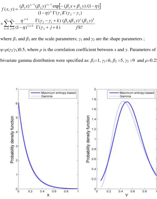
of different distances from the Gulf of Mexico ... 17 Figure 2. 7 Parent distributions for Monte Carlo simulation ... 23 Figure 2. 8 IDF curves for different durations ... 33 Figure 3. 1 Maximum entropy-based marginal PDFs and gamma marginal PDFs

for variables X and Y ... 49 Figure 3. 2 Comparison of maximum entropy-based joint distribution and bivariate

gamma distribution ... 51 Figure 3. 3 Boxplots of statistics of the calibration sample and generated data pairs 52 Figure 3. 4 Maximum entropy-based marginal PDFs and empirical histograms for

scaled May and June streamflow ... 55 Figure 3. 5 Contours of the maximum entropy-based PDF of scaled May and June

streamflow ... 56 Figure 3. 6 Boxplots of mean, standard deviation, skewness and lag-one correlation

of generated and historical data for simulation S1.. ... 57 Figure 3. 7 Absolute errors of mean, standard deviation, skewness and lag-one

Figure 3. 8 Boxplots of mean, standard deviation, skewness and lag-one correlation of generated and historical data for simulation S2 ... 60 Figure 3. 9 Boxplots of maximum and minimum values of generated and historical

data for simulation S1 and S2 ... 62 Figure 3. 10 Boxplots of kurtosis of historical and generated data ... 64 Figure 3. 11 Boxplots of ratio of drought, surplus and storage capacity statistics .... 65 Figure 4. 1 Empirical and theoretical distribution for May streamflow ... 77 Figure 4. 2 Empirical and theoretical distribution for September streamflow ... 78 Figure 4. 3 K-Plot of different copulas for May-June streamflow pairs ... 80 Figure 4. 4 K-Plot of different copulas for October-November streamflow pairs .... 81 Figure 4. 5 Comparison of observed monthly streamflow and a sequence of

generated monthly streamflow. ... 84 Figure 4. 6 Boxplots of basic statistics of generated and historical monthly

streamflow from the ECG method ... 86 Figure 4. 7 Boxplots of basic statistics of generated and historical annual

streamflow from two methods ... 87 Figure 4. 8 Boxplots of lag-four correlation of generated and historical monthly

streamflow from two methods ... 89 Figure 4. 9 Boxplots of inter-annual dependence of generated and historical monthly

streamflow from the EECG method. ... 90 Figure 5. 1 Illustration of four stations in Colorado River basin ... 104 Figure 5. 2 Marginal PDF of the annual streamflow at site 1 from entropy method

and entropy-copula method ... 107 Figure 5. 3 Scatter plot of observed streamflow (star) and generated streamflow

from entropy method (open circle) and entropy-copula method (dot) .... 109 Figure 5. 4 Boxplots of mean, standard deviation and skewness of annual

Figure 5. 5 Boxplots of maximum and minimum values of annual streamflow from entropy method and entropy-copula method ... 112 Figure 5. 6 Boxplots of Pearson, Keandall, and Spearman correlations of annual

streamflow pairs from entropy method and entropy-copula method. . .. 113 Figure 6. 1 Scatterplot of observed data and generated data from ME1 and ME2

distributions ... 125 Figure 6. 2 Comparison of empirical and theoretical probability for drought duration

and severity ... 126 Figure 6. 3 Empirical histograms and marginal PDFs from entropy-based ME2,

exponential and gamma distributions ... 128 Figure 6. 4 Empirical probabilities and theoretical probabilities from entropy-based

ME2, exponential and gamma distributions ... 130 Figure 6. 5 Contours of joint return period (years) of drought duration and severity

from entropy-based ME2 distribution ... 133 Figure 6. 6 Conditional return periods of drought duration and severity from

entropy-based ME2 distribution ... 134 Figure 7. 1 Monthly PDSI data of Climate Division 5 in Texas ... 146 Figure 7. 2 Empirical histograms and entropy-based probability density function .. 148 Figure 7. 3 Empirical and entropy-based cumulative distribution function ... 149 Figure 7. 4 Comparison of empirical and theoretical joint probability distributions 150 Figure 7. 5 Comparison of theoretical and empirical type I joint return period... 153 Figure 7. 6 Type I joint return period of drought duration and severity ... 154 Figure 7. 7 Type II joint return period of drought duration and severity ... 155 Figure 7. 8 Conditional return period for drought duration given drought severity

LIST OF TABLES

Page Table 2. 1 Median of estimated quantiles with random numbers generated from

the GEV distribution ... 24

Table 2. 2 RMSE of estimated quantiles with random numbers generated from the GEV distribution ... 25

Table 2. 3 Median of estimated quantiles with random numbers generated from the log-normal distribution with different skewness (k) ... 26

Table 2. 4 RMSE of estimated quantiles with random numbers generated from the log-normal distribution with different skewness (k) ... 27

Table 2. 5 Number of stations with the minimum RMSE from each distribution .... 30

Table 2. 6 Number of stations with the minimum RMSE for different climate zones and durations ... 31

Table 2. 7 Number of stations with the minimum RMSE for different distances from the sea and durations ... 32

Table 3. 1 Relative error (%) of statistics for each month for simulation S1 ... 59

Table 3. 2 Comparison of statistics of generated and observed streamflow of January and May for simulation S1 and S2 ... 61

Table 4. 1 Copulas with associated parameter space and Kendall’ tau ... 72

Table 4. 2 Statistics Sn and associated p-values for different streamflow pairs ... 83

Table 4. 3 Statistics Tn and associated p-values for different streamflow paris ... 83

Table 4. 4 Relative error (%) for simulated statistics of each month ... 86

Table 5. 1 Statistics of annual streamflow at four sites ... 104

Table 5. 2 Goodness of fit test for statistics Sn and Tn with associated p values for different streamflow pairs . ... 108

Table 5. 3 Relative error (%) of statistics generated from entropy method and

entropy-copula method ... 111 Table 5. 4 Relative error (%) of different dependence measure from entropy method and entropy-copula method ... 114 Table 6. 1 Return period of drought duration and severity. ... 132 Table 7. 1 Number of cases of ENT distribution with the best performance for

different types of datasets ... 144 Table 7. 2 RMSE and AIC values of different distributions for the case study ... 146 Table 7. 3 Univariate return period for drought duration and severity ... 151

CHAPTER I INTRODUCTION

Characterization of hydrologic events, such as rainfall, streamflow and drought, is needed for water resources planning and management. Due to the stochastic nature of hydrologic phenomena, stochastic methods are commonly used. For rainfall analysis, a proper distribution is generally needed to investigate statistical properties of rainfall quantiles and extrapolate beyond the available data for engineering purposes. For streamflow simulation, synthetic streamflow with statistical properties similar to those historical streamflows are required for evaluation of alternative designs and policies against the range of sequences that are likely to occur in the future. A joint distribution with different marginal distributions is generally needed to characterize the correlation between drought variables and distribution property of individual drought variables to analyze return periods corresponding to some occurrence levels of drought events.

A proper characterization of hydrologic events necessitates the consideration of uncertainty in the estimation from limited observations. Entropy theory defines a measure of uncertainty or information and thus provides a proper way to characterize hydrologic events with stochastic nature. Application of entropy theory to rainfall analysis, streamflow simulation and drought analysis constitutes the objective of this study.

Rainfall frequency analysis is needed for the construction of intensity-duration- ____________

frequency (IDF) curves which are used for engineering design of drainage systems, culverts, roadways and parking lots. Extreme values, such as the annual rainfall maxima, are generally used for frequency analysis. The generalized extreme value (GEV)

distribution, which is based on the extreme value theory, has been commonly used for modeling extreme rainfall in different states. However, there are a variety of studies for extreme rainfall analysis in which other distributions have often been employed.

Extreme rainfall exhibits different properties for different durations and in different regions. The question is: what is the effect of time duration, climate zone and the distance from the Gulf of Mexico on the frequency distribution of annual rainfall maxima? In this study, the State of Texas was selected as the study area and we try to answer these three questions to provide an insight into the analysis of extreme rainfall.

In chapter II, the change in the form of the annual rainfall maximum frequency distribution with changes in time duration, climate zone, and distance from the Gulf of Mexico is investigated. An entropy based distribution is then proposed to model the annual rainfall maxima. The performance of the proposed method is compared with the commonly used GEV distribution based on the synthetic data and real observations.

Streamflow is a component of a variety of hydrologic analysis, such as the reservoir planning and operation. Since historical streamflow does not allow for the evaluation of alternative designs and policies against the range of sequences that are likely to occur in the future, synthetic streamflow data are useful in water resources studies. It is desired that synthetic streamflow is similar to historical streamflow and preserves moment statistics (such as mean, standard deviation, and skewness), and

dependence structure (such as lag-one correlation). For traditional methods, the Gaussian assumption is generally needed for parametric methods in which transformation

techniques are employed. However, some problems arise, such as the generation of negative values due to the Gaussian assumption and the bias in simulated statistics due to the transformation techniques. In addition, the lag-one correlation (or Pearson

product-moment correlation coefficient) only measures the linear dependence of random variables, which may not be adequate in reality. Moreover, some unusual features, such as the bimodality, may exist in the probability density function of streamflow data. It is difficult for the commonly used parametric approach to represent these features. Though the mixed distribution can be used to resolve the bimodality, bias in the statistics of streamflow may occur.

In Chapter III, an entropy based method is proposed for monthly streamflow simulation. With the joint distribution of monthly streamflows of two adjacent months derived using the entropy theory, monthly streamflow is then generated by sequential sampling from the conditional distribution. The proposed entropy-based method does not rely on the assumption of the marginal distributions to be normal and data

transformation is not needed. Therefore, issues with the data transformation existing in the commonly used parametric approaches can be avoided. This method can be extended to model more statistics of the underlying streamflow data if needed. The disadvantage of the entropy based method is that the method will be computationally cumbersome when more statistics need to be modeled.

In Chapter IV, an entropy-copula method is proposed for single-site monthly streamflow simulation in which the joint distribution is constructed using the copula theory with the marginal distribution derived using the entropy theory. The entropy-copula method simplifies the entropy method for monthly streamflow simulation in that less number of parameters needs to be estimated simultaneously. Furthermore, the entropy-copula method is also capable of modeling the nonlinear dependence of streamflow between different months due to the copula component. The proposed entropy-copula method is also extended with an aggregated variable to guide the

sequential simulation to improve the preservation of high-order correlation and preserve the inter-annual dependence of monthly streamflow.

In Chapter V, both the entropy method and entropy-copula methods are extended to higher dimension for multi-site annual streamflow simulation. The difference between two methods lies in modeling the dependence structure of streamflow. For the entropy method, the joint constraints are used for modeling the dependence while the copula is used for modeling the dependence for the entropy-copula method. Application of the proposed method based on annual streamflow from four stations in Colorado River basin illustrates the effectiveness and difference of the entropy method and entropy-copula method for streamflow simulation.

Drought analysis is important for water resources planning and management. A drought event can be characterized with certain properties, such as duration and severity. Drought duration and severity, assumed as random variables, have been commonly used for drought analysis and a traditional way for characterizing drought is fitting an

empirical distribution to drought duration and severity. The joint distribution is needed to model the correlation between drought variables. Traditional joint distributions that have been applied for drought analysis generally assume that the marginal distribution is of the same type. The copula method has been employed extensively for modeling drought duration and severity with the attractive property that the marginal distribution can be of different forms. However, the marginal distributions are often derived by empirically fitting to the data.

In Chapter VI, an entropy based distribution is proposed for constructing the joint distribution of drought variable. The feature of the proposed entropy-based distribution is that the marginal distributions can be of different forms. The advantage of the

proposed method is the marginal distribution can be derived with whatever is known from observations and is not restricted by the empirical forms of distributions.

In Chapter VII, an entropy-copula method is proposed for constructing a joint distribution for drought analysis. Flexible distribution forms can be derived with the entropy method and the commonly used distributions can also be derived as special cases of the entropy based distribution. A variety of copulas have been proposed that are capable of modeling different dependence structures. The joint distribution constructed with the copula method with the marginal distributions derived from the entropy theory is expected to be capable of modeling drought variables separately and jointly.

CHAPTER II

ENTROPY BASED METHOD FOR RAINFALL ANALYSIS

2.1 Introduction

Rainfall frequency analysis is used for constructing intensity-duration-frequency (IDF) curves which are needed for a range of hydrologic designs, including drainage systems, culverts, roadways, parking lots, runways, and so on. Extreme rainfall values, such as annual rainfall maxima, are of interest in modeling floods and quantifying the effect of climate change. From the fitted distribution, statistical properties of extreme rainfall values can be investigated and extrapolated beyond the available data for engineering purposes.

The generalized extreme value (GEV) distribution is one of the frequently employed probability distributions for modeling and characterizing extreme values. Derived from the extreme value theory, it is a three-parameter distribution encompassing three classes of distributions, namely, Gumbel, Frechet and Weibull. This distribution has been used for extreme rainfall frequency analysis in different areas of the world. Schaefer [1990] used the GEV distribution for frequency analysis of annual rainfall maxima of durations of 2 h, 6 h and 24 h for the state of Washington. Huff and Angel [1992] selected the GEV distribution to model the distribution of annual rainfall maxima for durations from 5 minutes to 10 days in mid-western United States. Parrett [1997] also used the GEV distribution to construct dimensionless frequency curves of annual

rainfall maxima of durations of 2 h, 6 h and 24 h within each region in Montana. Using the L-moment ratio diagram, Asquith [1998] determined that the GEV distribution was an appropriate distribution for modeling the distribution of annual maxima for durations from 1 to 7 days. Alila [1999] showed that the annual rainfall extremes for durations from 5 minutes to 24 hours in Canada were better described by the GEV distribution than other distributions, such as the generalized logistic (GLO), Pearson type 3 (P3) and EV1 distributions.

Extreme rainfall exhibits different properties for different durations in different regions. Analysis of rainfall characteristics is important for choosing a suitable rainfall distribution and consequently estimating rainfall quantiles. Therefore, the objective of this study is to investigate the change in the form of the annual rainfall maxima frequency distribution with changes in time duration, climate zone, and distance from the Gulf of Mexico; and then derive an entropy-based distribution that is sufficiently flexible for characterizing rainfall distributions for different durations in different climatic regions or at different distances from the sea. The performance of the proposed entropy based distribution is assessed using synthetic data through Monte Carlo

simulation and real observations and is shown to be a promising alternative distribution to the commonly used GEV distribution for modeling extreme rainfall values, especially for observations with high skewness.

The study is organized as follows. In section 2.2, the change in form of empirical distribution of annual rainfall maxima is investigated. Using the entropy theory, a

is assessed by comparing with the GEV distribution in Section 2.4. After the application of the proposed entropy based distribution in section 2.5, conclusions are given in section 2.6.

2.2 Empirical frequency distribution 2.2.1 Study area

Figure 2. 1 Regions of climate zones in Texas ([Larkin and Bomar, 1983]).

The area selected for this study is the state of Texas (longitude: 93° 31' W to 106° 38' W, latitude: 25° 50' N to 36° 30' N). The climate of Texas is strongly influenced by physical features including the Gulf of Mexico. The passage of frontal systems from northwest and the moist air moving inland from the Gulf of Mexico are the two

the most important factor that determines the regional climatic differences in Texas [North et al., 1995].

There are three major types of climate in Texas which are classified as

Continental, Mountain and Modified Marine with no clearly distinguishable boundaries, while the modified marine zone is further classified into four “subtropical” zones

[Larkin and Bomar, 1983; Narasimhan et al., 2008], as shown in Figure 2. 1.The

Mountain climate is dominant in several mountains of the Trans-Pecos region and is not included in this study. The different climate zones of the Continental and Modified Marine climate are abbreviated as Continental Steppe (CS), Subtropical Arid (SA), Subtropical Humid (SH), Sub-tropical Sub-Humid (SSH) and Sub-Tropical Steppe zone (SST). In addition, the U.S. National Weather Service divided Texas into 10 climate divisions (including Upper Coast, East Texas, High Plain, Trans-Pecos and so on ) which are used accordingly in this study.

2.2.2 Data description

Data for 15-minute, hourly, and daily duration for National Weather Service (NWS) stations, as shown in Figure 2. 2, were obtained from the National Climatic Data Center (http://www.ncdc.noaa.gov). The 15 and 45-minute annual maxima were

compiled from the 15-minute data. Likewise, the rainfall data for different hourly durations (1-hour and 12-hour) and daily durations (1-day, 7-day and 30-day) were compiled from hourly and daily data, respectively. Annual rainfall maxima data were then obtained from these rainfall data for different durations.

Figure 2. 2 Rainfall stations used in this study.

2.2.3 Change in distribution form with time duration

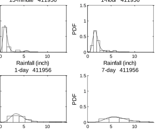
Histograms of annual rainfall maxima of different durations were prepared for all raingage stations used in this study and those for a sample station (411956) are shown in Figure 2. 3. It was observed that frequency distributions for short durations were more skewed with sharp peaks but tended to be less skewed with increase in the duration. For example, annual rainfall maxima data for station 411956 had a skewness value of 2.7 for 15-minute data but 1.1 for 30-day data (not shown).

0 5 10 0 0.5 1 1.5 Rainfall (inch) 15-minute 411956 P D F 0 5 10 0 0.5 1 1.5 Rainfall (inch) 1-hour 411956 P D F 0 5 10 0 0.5 1 1.5 Rainfall (inch) 1-day 411956 P D F 0 5 10 0 0.5 1 1.5 Rainfall (inch) 7-day 411956 P D F

Figure 2. 3 Histograms and probability density functions of rainfall data of different durations (for station 411956 in the Subtropical Humid (SH) climate

zone).

To further show this characteristic, the boxplot of skewness values for 40 datasets of different durations is demonstrated in Figure 2. 4. For example, the 75 percentile of skewness of the 15 minute duration was around 3.2 while that for the 30-day duration was 1.2. This is partly because for short duration like 15 minutes, a large amount of rainfall may occur within a short time in certain cases exhibiting large

skewness while for long durations, like 30 days, the data is averaged and thus it exhibits less skewness.

-0.5 0 0.5 1 1.5 2 2.5 3 3.5 4 4.5

15-minute 45-minute 1-hour 12-hour 1-day 7-day 30-day

S ke w n e ss

Figure 2. 4 Skewness of annual rainfall maxima of different durations (40 datasets for each duration).

2.2.4 Change in distribution form with climatic zone

Subtropical humid zone (SH)

The subtropical humid (SH) zone lies in the eastern part of Texas which is mostly noted for warm summers [Larkin and Bomar, 1983]. Ten stations were selected for the study. This zone includes most parts of Upper Coast and East Texas division. There are four rainfall generating mechanisms that exist in the Upper Coast area, leading to varying patterns from year to year as one or more of these controls change: in May the

typical thunderstorm pattern is expected slightly inland while the belt of maximum activity is along the coast by July; in September tropical disturbances can cause very heavy rains for some years, while in December frontal activity affects the region

[National Fibers Information Center, 1987]. The East Texas division is characterized by a fairly uniform seasonal rainfall with slight maxima occurring in May and December and there is little variation in the weather in the summer season, because the influence of the Gulf of Mexico is dominant [ National Fibers Information Center, 1987]. The most widespread and lengthy precipitation periods in East Texas during spring and autumn occur when the cold air forms a barrier, forcing the overriding moist Gulf air to be deflected upward where it cools and condenses [Carr, 1967].

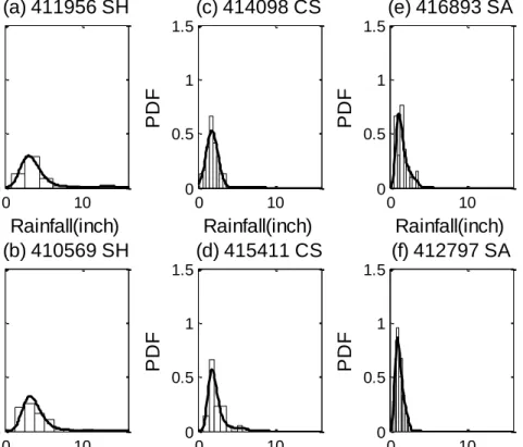
For two stations 411956 and 410569, the histograms are shown in Figure 2. 5 (a) and (b) for 12-hour annual rainfall maxima. It can be seen that frequency distributions are smooth for the data of this duration. This region is along the coast and the rainfall pattern is affected by the Gulf of Mexico. Since the proximity to the coast is the most determining factor for regional climate differences [North et al., 1995], the reason for this frequency distribution pattern may be due to the moderating moisture from the Gulf of Mexico.

Subtropical sub-humid zone (SSH)

The subtropical sub-humid (SSH) zone is located in the central part of Texas which is characterized by hot summers and dry winters [Larkin and Bomar, 1983]. No clear pattern was discernible from the frequency distribution of several stations in this climate zone.

0 10 0 0.5 1 1.5 Rainfall(inch) (a) 411956 SH P D F 0 10 0 0.5 1 1.5 Rainfall(inch) (c) 414098 CS P D F 0 10 0 0.5 1 1.5 Rainfall(inch) (e) 416893 SA P D F 0 10 0 0.5 1 1.5 Rainfall(inch) (b) 410569 SH P D F 0 10 0 0.5 1 1.5 Rainfall(inch) (d) 415411 CS P D F 0 10 0 0.5 1 1.5 Rainfall(inch) (f) 412797 SA P D F

Figure 2. 5 Histograms and probability density functions of 12-hour rainfall data of different climate zones.

Continental steppe zone (CS)

The continental steppe (CS) zone lies in the northwestern part of Texas and includes the regions similar to the High Plain division. The rainfall amount increases steadily through spring and reaches a maximum in May or June, while the thunderstorm activity is also on the rise during the spring season [National Fibers Information Center, 1987]. In this region, summer is the wet season and thunderstorms are numerous in June and July but begin to decrease in August. Two stations 414098 and 415411 were used for analysis and the histograms for 12-hour annual rainfall maxima are shown in Figure

2. 5 (c) and (d). The frequency distributions in this part are relatively sharp, compared with those from the SH climate zone. The reason may be that the maximum rainfall mainly comes from the thunderstorms during the summer season.

Subtropical Arid zone (SA)

The subtropical arid zone lies in the extreme western part of Texas and includes the region similar to the Pecos division. The basin and plateau region of the Trans-Pecos features a subtropical arid climate, which is marked by summertime rainfall anomalies of the mountain relief [Larkin and Bomar, 1983]. Rainfall reaches its maximum in July and in summer, where the rain comes mainly from thunderstorms, often affected by local topography [National Fibers Information Center,1987]. In the Trans-Pecos region, the biggest percentage of rainfall occurring in this area is due to convective showers and thundershower activity, while the thundershower activity is the primary contributor of rainfall during late summer and early autumn months [Carr, 1967]. Two stations 416893 and 412797 were selected for analysis and the histograms for the 12-hour annual rainfall maxima are shown in Figure 2. 5 (e) and (f). The

frequency distributions were relatively sharp compared with those from the SH climate zone. The reason for the variation of rainfall may be that the heavy rainfall in SA is mainly produced due to the convective shower and thundershower activity.

Subtropical steppe zone (SST)

From the mid-Rio Grande Valley to the Pecos Valley, the broad swath of Texas has a subtropical Steppe (SST) climate and is typified by semi-arid to arid conditions

[Larkin and Bomar, 1983]. No clear pattern of frequency distributions in this zone was found from the data of several stations.

In general, frequency distributions for regions in extremely northern and western parts (or the CS and SA climate zones) were sharp; however, those for the regions in the southeast near the Gulf Mexico (or the SH climate zones) were rather smooth. In

general, frequency distributions became smoother from northwest to southeast. Although only a few of the possible mechanisms of rainfall in each region were investigated, the analysis provided an insight into the reason for the specific rainfall frequency

distribution pattern in each climate region.

2.2.5 Influence of the distance from the sea (or the Gulf of Mexico)

The Gulf of Mexico is particularly important for the climate of Texas, as it provides the source of moisture and modulates the average seasonal and diurnal cycles, particularly in the coastal regions [North et al., 1995]. In general, the average annual rainfall decreases with increasing distance from the Gulf of Mexico.

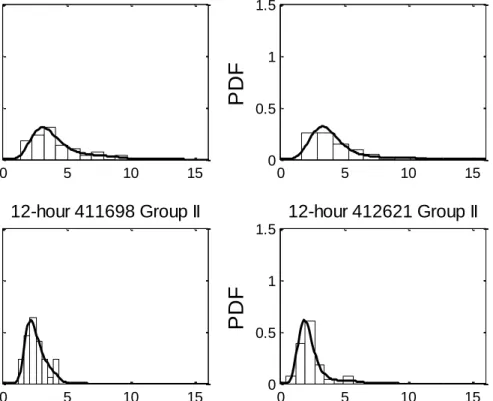
To assess the effect of the Gulf of Mexico on the distribution of annual rainfall maxima, 20 stations were selected and divided into two groups each with 10 stations according to the distance from the Gulf of Mexico. The histograms of 12-hour

maximum rainfall for four sample stations are shown in Figure 2. 6. It can be seen that the frequency distributions in group II (more than 250 miles away from the Gulf) are not as smooth as those in group I (within 60 miles from the Gulf), which are located along the coast. The smoothness of frequency distributions in Group I is partly due to the closeness of rainfall stations to the Gulf of Mexico. The effect of Gulf of Mexico is

reduced with the distance and the topology factor may also play an important role for the rainfall generating mechanism. The frequency distribution pattern for the two stations in Group II may be due to the mixed effect of the Gulf of Mexico and topology.

0 5 10 15 0 0.5 1 1.5 12-hour 414309 Group I

P

D

F

P

D

F

P

D

F

P

D

F

Figure 2. 6 Histograms and probability density functions of 12-hour rainfall data of different distances from the Gulf of Mexico (414309, 60 miles; 412015, 20 miles;

411698, 480 miles; 412621, 450 miles ).

It is clear that the probability distribution varies with time duration, climate zone and distance from the sea (or Gulf of Mexico). The question arises if a probability

distribution that can accommodate the effect of these factors. This is addressed in what follows.

2.3 Annual maximum rainfall distribution using entropy theory 2.3.1 Derivation of distribution

Let the annual maximum rainfall for a given duration be represented as a continuous random variable X є [a, b] with a probability density function (PDF), f(x). For f(x), the Shannon entropy E can be defined as [Shannon, 1948; Shannon and Weaver, 1949]:



where x is a value of random variable X with lower limit a and upper limit b. Jaynes [1957] developed the principle of maximum entropy (POME) which states that the probability density function should be selected among all the distributions with the maximum entropy subjected the given constraints. The constraints can be expressed in general form as:

) ( ) ( ) ( r b a r x f x dx E g g



where the function gr(x) in equation (2.2) is the known function with g0(x)=1; E(gr) is the

r-th expected value obtained from observations with g0=1; m is the number of constraints.

The maximum entropy based probability density function can then be obtained by maximizing the entropy in equation (2.1), subject to equations (2.2) using the method of Lagrange multipliers, as [Kesavan and Kapur, 1992]:

)] ( )... ( ) ( exp[ ) (x _{0 1}g₁ x ₂g₂ x g x f     _{m m} (2.3)

where λr (r=0, 1,…, m) are the Lagrange multipliers.

2.3.2 Maximum entropy distribution with moments as constraints

Moments can be used for the reconstruction of density based on maximum entropy [Mead and Papanicolaou, 1984]. With the first four moments as constraints, the maximum entropy-based probability density function (denoted as ENT4) defined on the interval [a, b], with the function g(x) in equation (2.2) expressed as gi(x)=xi (i=1, 2, 3 and

4) , can be expressed as:

) exp( ) ( 4 4 3 3 2 2 1 0 x x x x x f       (2.4)

In this study, the lower bound of the interval a is set to be zero, while the upper bound b was set to be 20 times the observed maximum value. Since higher moments are involved in this distribution, a relatively large datasets would be needed for the accuracy of the moment estimation.

With the first four moments as constraints, the skewness, kurtosis and multiple modes can be included in the resulting maximum entropy-based distribution [Zellner and Highfield, 1988]. Each maximum of the polynomial inside the exponential corresponds to one mode and thus the multiple modes may exist in the maximum distribution [Smith, 1993]. Matz [1978] developed a new algorithm for the maximum likelihood estimate of this distribution and showed its good performance in characterizing features of empirical distributions, including the bi-modal. Comparing this distribution with the Pearson distribution, Zellner and Highfield [1988] showed that it was comparable with the

Pearson distribution while provided a better fit for small sample size, especially at the tails. Smith [1993] used the maximum entropy-based distribution with moments as constraints for decision analysis to construct the distribution of value lottery and showed the distribution with first four moments as constraints performed well.

In this study, the entropy based distribution in equation (2.4) was proposed as an alternative for modeling extreme rainfall values. In addition, the entropy distribution with the first three moments as constraint was also selected as the candidate for modeling extreme rainfall values. From equation (2.3), this distribution with three parameters (denoted as ENT3) can be expressed as:

) exp( ) ( 3 3 2 2 1 0 x x x x f      (2.5) 2.3.3 Estimation of parameters

The Lagrange multipliers of equation (2.4) has to be determined using equations (2.2) where E(gr)(r=1, 2, 3, 4) are the expectation of the first four non-central moments.

Generally the analytical solution does not exist and the numerical estimation of the Lagrange multipliers is needed. To that end, one can maximize the function [Mead and Papanicolaou, 1984; Wu, 2003]:









i H       1 ) 0 ( ) 1 ( λ λ r=1, 2, 3, 4 ( (2.7) where the gradient Г is expressed as:

, ) ( ) ( exp 4 0 dx x g x g g b a r i r r i i





4 3, 2, 1, = , , ) ( ) ( exp ) ( ) ( exp ) ( ) ( ) ( exp 4 0 4 0 4 0 , j i dx x g x g dx x g x g dx x g x g x g H b a r j r r b a r i r r b a r i j r r j i













To quantify the performance of the proposed distribution in modeling the extreme rainfall quantiles, the root mean square error (RMSE) was used defined as:



estimated quantile from the fitted distribution corresponding to the empirical non-exceedance probabilities estimated from the plotting position formula. In this study, the Gringorten plotting position formula is used defined as [Gringorten, 1963]:

12 . 0 44 . 0    n i P (2.11) where i is the rank of the observed values and n is the length of the observed data.

2.4.2 Synthetic data from known distribution

Monte Carlo experiments were first carried out to compare the quantiles

estimated from the GEV, ENT4 and ENT3 distributions. Two Monte Carlo simulations were conducted with random numbers generated from the known GEV and lognormal distributions. Random numbers of three different lengths (namely, 40, 70 and 100) were generated, which were used to approximate the record length of the 15-minutes, hourly and daily rainfall data in this study. For the first simulation (S1), the quantiles

corresponding to different return periods (T = 5, 10, 25, 50, 100, 200 years) were first assessed with the random number generated from the GEV distribution. For the second simulation (S2), the quantiles corresponding to relatively long return period (T=100 and 200 years) from the three distributions were assessed with the synthetic data generated from log-normal distribution with different skewness values.

Random number from Generalized Extreme Value distribution (GEV)

The generalized extreme value (GEV) distribution has been applied extensively in hydrology for extreme rainfall analysis. Its probability density function is defined as:

                              _       _      0 , ) exp( exp 1 0 , ) ( 1 exp ) ( 1 1 ) , , ; ( / 1 1 / 1 k u x u x k u x k u x k k x f k k         (2.12)

where k, σ and u are the shape, scale and location parameter. In this study, the MATLAB function gevfit was used for the parameter estimation of the GEV distribution with maximum likelihood method.

0 1 2 3 4 5 6 0 0.5 1 1.5 x (a) P D F 0 1 2 3 4 5 6 0 0.5 1 x (b) P D F s=1 s=2 s=2.5 s=3

Figure 2. 7 Parent distributions for Monte Carlo simulation. (a) GEV distribution; (b) Lognormal distribution with different skewness (s).

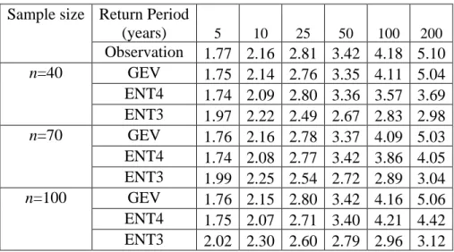
1000 datasets of random numbers with different sample sizes (n=40, 70, 100) were generated from this parent distribution. The GEV, ENT4 and ENT3 distributions were then fitted to these datasets and the quantiles corresponding to different return periods were obtained. Parameters (k, σ , u) of the parent distribution were assigned as (0.3,0.3,1.2) and the probability density function is shown in Figure 2. 7

The median and the RMSE values of the estimated quantiles for simulation S1 are shown in Table 2. 1. From the median values, it can be seen that for short return periods (T ≤ 50 years), the median values from the ENT4 and GEV distributions were close to

each other for each sample size. For example, for sample size n=100, the median values from GEV and ENT4 for return period 50 years were 3.42 and 3.40, respectively, while the observed value was 3.42.

Table 2. 1 Median of estimated quantiles with random numbers generated from the GEV distribution.

Sample size Return Period

(years) 5 10 25 50 100 200 Observation 1.77 2.16 2.81 3.42 4.18 5.10 n=40 GEV 1.75 2.14 2.76 3.35 4.11 5.04 ENT4 1.74 2.09 2.80 3.36 3.57 3.69 ENT3 1.97 2.22 2.49 2.67 2.83 2.98 n=70 GEV 1.76 2.16 2.78 3.37 4.09 5.03 ENT4 1.74 2.08 2.77 3.42 3.86 4.05 ENT3 1.99 2.25 2.54 2.72 2.89 3.04 n=100 GEV 1.76 2.15 2.80 3.42 4.16 5.06 ENT4 1.75 2.07 2.71 3.40 4.21 4.42 ENT3 2.02 2.30 2.60 2.79 2.96 3.12

The RMSE values of the estimated quantiles for simulation S1 are shown in Table 2. 2. Generally the RMSE values of the ENT4 distribution were slightly larger than those of the GEV distribution, however, these results were acceptable. For the quantiles

corresponding to the relatively long return periods (100 and 200 years), the median quantile from the ENT4 distribution is slightly underestimated, while that from the GEV distribution was close to the true value. This is not unexpected, since the random

numbers were generated from the GEV distribution and then the GEV distribution was fitted. Generally ENT4 modeled the data generated from the GEV distribution well,

especially when the sample size was relatively large. The ENT3 distribution also estimated the quantiles relatively well for short periods (T ≤ 25 years), while it did not model the quantiles well corresponding to relatively long return periods (T ≥ 50 years).

Table 2. 2 RMSE of estimated quantiles with random numbers generated from the GEV distribution.

Sample size Distribution Return Period (years)

5 10 25 50 100 200 n=40 GEV 0.14 0.25 0.55 0.96 1.64 2.73 ENT4 0.15 0.28 0.77 1.70 1.74 2.00 ENT3 _{0.38 0.47 0.66 0.95 1.43 2.12} n=70 GEV 0.10 0.19 0.40 0.69 1.15 1.86 ENT4 0.12 0.22 0.52 1.02 2.28 2.38 ENT3 0.35 0.41 0.59 0.91 1.45 2.36 n=100 GEV _{0.09 0.16 0.34 0.57 0.93 1.46} ENT4 0.11 0.18 0.42 0.97 2.67 2.74 ENT3 0.36 0.44 0.62 0.90 1.37 2.05

Random number from log-normal distribution

The probability density function of the log-normal distribution can be expressed as: 2 2 2 ₂ ) (ln 2 1 ) (   u x e x x f    (2.13) where u is the mean in the log-scale and σ2

is the variance in the real scale. The skewness coefficient s is related with the variance σ2 _{as s=[exp(σ}2_)+2][exp(σ2

this study, the MATLAB function lognfit was used for the parameter estimation of the log-normal distribution with maximum likelihood method.

Table 2. 3 Median of estimated quantiles with random numbers generated from the log-normal distribution with different skewness (k).

Sample Size Skewness k=1 k=2 k=2.5 k=3

Quantile x100 x200 x100 x200 x100 x200 x100 x200 Observation 2.80 3.03 4.87 5.59 5.99 7.03 7.13 8.53 n=40 GEV 2.73 2.95 5.12 6.02 6.48 7.94 7.84 10.00 ENT 2.61 2.72 4.34 4.54 5.15 5.39 5.93 6.21 ENT3 2.44 2.55 3.85 4.11 4.62 4.97 5.35 5.81 n=70 GEV 2.77 2.99 5.07 5.98 6.57 8.09 8.25 10.57 ENT 2.69 2.83 4.60 4.88 5.58 5.91 6.83 7.26 ENT3 2.46 2.58 3.88 4.14 4.75 5.12 5.78 6.30 n=100 GEV 2.80 3.01 5.13 6.08 6.60 8.14 8.34 10.66 ENT 2.74 2.88 4.77 5.05 5.92 6.30 7.19 7.70 ENT3 2.48 2.59 3.90 4.17 4.81 5.21 5.85 6.42

1000 datasets of random numbers with different sample sizes (n=40, 70 and 100) with different skewness 1, 2 , 2.5 and 3 were generated from log-normal distribution and used for comparison. Parameter u is assigned as 0.3 while the standard deviations

corresponding to different skeweness values were assigned as 0.31, 0.55, 0.64 and 0.72, respectively. The PDFs for the parent distributions with these parameters are shown in Figure 2. 7 (b). The objective of this simulation was to show the performance of these distributions in modeling data with different skewness. The median and RMSE values of the estimated quantiles for return period 100 and 200 years (denoted as x100 and x200) corresponding to non-exceedance probability 0.99 and 0.995 are shown in Table 2. 3 and Table 2. 4.

Table 2. 4 RMSE of estimated quantiles with random numbers generated from the log-normal distribution with different skewness (k).

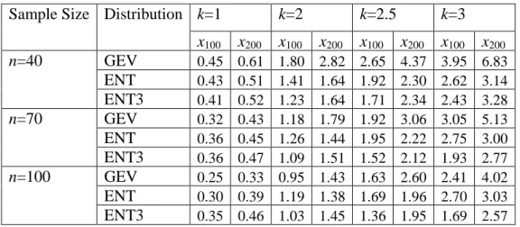
Sample Size Distribution k=1 k=2 k=2.5 k=3 x100 x200 x100 x200 x100 x200 x100 x200 n=40 GEV 0.45 0.61 1.80 2.82 2.65 4.37 3.95 6.83 ENT 0.43 0.51 1.41 1.64 1.92 2.30 2.62 3.14 ENT3 0.41 0.52 1.23 1.64 1.71 2.34 2.43 3.28 n=70 GEV 0.32 0.43 1.18 1.79 1.92 3.06 3.05 5.13 ENT 0.36 0.45 1.26 1.44 1.95 2.22 2.75 3.00 ENT3 0.36 0.47 1.09 1.51 1.52 2.12 1.93 2.77 n=100 GEV 0.25 0.33 0.95 1.43 1.63 2.60 2.41 4.02 ENT 0.30 0.39 1.19 1.38 1.69 1.96 2.70 3.03 ENT3 0.35 0.46 1.03 1.45 1.36 1.95 1.69 2.57

For the case with skewness k=1, the median quantiles from the ENT4 distribution was not as close to the observed values as from the GEV distribution. However, the difference of the estimated median from GEV and ENT4 was relatively small, especially for relatively large sample sizes. For example, for n=100, the median values from GEV and ENT4 were 2.80 and 2.74 with the observed value being 2.80. Generally the RMSE values of the two distributions were close to each other. For example, the RMSE of GEV and ENT4 for x200 were 0.43 and 0.45, respectively, for n=70. The performance of ENT4 is improved with the increase of sample size. Generally the performance of ENT4 and GEV were comparable in this case.

For skewness values of k=2 and 2.5, the median values from GEV were

overestimated while those from ENT4 were slightly underestimated. When the sample size was relatively small (n=40), the GEV distribution performs slightly better than the ENT4 distribution for the median values. However, the RMSE value from the GEV is

higher than the ENT4 distribution. When the sample size was relatively large (n=100), the ENT4 distribution generally performed better than the GEV distribution for the median value, while their performance was comparable for the RMSE values. For example, for the case with k=2.5 and sample size n=100, the median values from GEV and ENT4 corresponding to the 100 year return period were 6.60 and 5.92 while the true value was 5.99. The corresponding RMSE values for GEV and ENT4 were, respectively, 1.63 and 1.69, which are comparable. The performance of the ENT4 distribution

improved with the increase of sample size.

For the skewness k=3, the median value estimated from GEV was overestimated significantly, while ENT4 still performed relatively well for estimating quantiles, especially when the sample size was relatively large. For example, the true quantile corresponding to the 100 year return period was 7.13, while the quantiles from GEV and ENT4 with sample size (n=70) were 8.25 and 6.83, respectively. The corresponding RMSE values were 3.05 and 2.75, indicating that ENT4 performed relatively better.

Though the RMSE values from ENT3 distribution was comparable with the ENT4 distribution and sometimes even smaller than ENT4 distribution, generally the median value from ENT3 was underestimated significantly for each sample size with different skewness. These results showed that generally ENT3 did not perform as well as the GEV and ENT4 distributions and was not suitable for modeling extreme values. Summary

The Month Carlo simulation S1 showed that generally the ENT4 distribution was comparable to the GEV distribution in modeling extreme rainfall values. Since the GEV

distribution has been extensively applied for modeling extreme values, the results from the first simulation S1 showed that the ENT4 distribution would also be a candidate for modeling the extreme values. The Monte Carlo simulation S2 showed that the

performance of the ENT4 distribution was comparable with GEV for low skewness , especially when the sample sizes were relatively large (n ≥ 70). When the skewness was relatively high ( k ≥ 2), the ENT4 distribution performed relatively better than the GEV distribution for estimating quantiles corresponding to relatively long return periods, especially when the sample size was large. Botero and Francés [2010] also found that the GEV distribution led to large errors for quantile estimation corresponding to long return periods for high skewness.

Synthetic data from other distributions (e.g., gamma distribution) were also used for comparison and generally similar results were obtained (not presented). Thus it can be concluded from the Monte Carlo simulation that generally the ENT4 distribution provided an alternative to the commonly used GEV distribution and should be preferable for observations with higher skewness. The ENT3 distribution was not suitable for modeling extreme values.

2.4.3 Real rainfall data from observation

To further compare the performance of the GEV distribution and ENT4 distribution, the observed rainfall data from 40 stations for different time duration (15-min, 45-(15-min, 1-hour, 12-hour, 1-day, 7-day and 30-day) were also used. The two distributions were compared based on empirical and theoretical quantiles according to the RMSE measure. The number of stations for each distribution performing the best

(with the least RMSE) is shown in Table 2. 5. For all durations, the ENT4 distribution performed the best for the largest number of stations. For example, for the annual

rainfall maxima of the 12-hour duration, the ENT4 distribution performed the best for 36 stations according to RMSE. From these results, it can be seen that the ENT4

distribution would be a good candidate for modeling annual rainfall maxima.

Table 2. 5 Number of stations with the minimum RMSE from each distribution.

Duration ENT GEV ENT3

15-minute 33 7 0 45-minute 36 3 1 1-hour 36 4 0 12-hour 36 4 0 1-day 33 7 0 7-day 32 8 0 30-day 32 8 0

2.5 Application of the entropy based distribution

The entropy-based distribution was used to fit the rainfall data in section 2.2, as shown in Figure 2. 3, Figure 2. 5 and Figure 2. 6, together with the empirical histograms as shown in the previous section. These figures show that the entropy-based distribution (ENT4) fitted the empirical histograms well for the rainfall data of different durations, climate zones and different distances from the Gulf.

The GEV distribution was also applied here for further comparison with the ENT4 distribution. For each duration (15-min, 45-min, 1-hour, 12-hour, 1-day, 7-day and 30-day), 10 stations were used in each climate zone (except that for the SA climate

zone, 6 stations were used for 15-minute and 45-minute duration due to data limitation). The number of stations that ENT4 or GEV performed better in different climate zones is shown in Table 2. 6. Taking the result in the CS climate zone as an example, the ENT4 distribution performed better for all durations for at least 8 out of 10 datasets.

Table 2. 6 Number of stations with the minimum RMSE for different climate zones and durations.

Duration CS SAa SH

ENT GEV ENT GEV ENT GEV

15-minute 9 1 4 2 10 0 45-minutes 10 0 6 0 9 1 1-hour 9 1 9 1 10 0 12-hour _{9 1 10 0 8 2} 1-day 8 2 7 3 9 1 7-day 8 2 8 2 7 3 30-day 8 2 8 2 7 3 a

For SA climate region of 15 and 45-minute data, only 6 stations are selected due to data limitation

The ENT4 distribution was also compared with the GEV distribution for different distances from the sea (Group I and Group II) with 10 stations in each group. There were not enough stations with a relatively long record of 15 minutes data in Group I and thus only the hourly (1-hour and 12-hour) and daily data (1-day, 7-day and 30-day) were used for comparison. The number of cases that ENT4 performed better than GEV for the two groups is shown in Table 2. 7. It can be seen that generally the ENT4 distribution performed better than the GEV distribution. Taking the 1 hour data as an

example, the ENT4 distribution had less RMSE for 10 and 8 cases for Groups I and II, respectively.

Table 2. 7 Number of stations with the minimum RMSE for different distances from the sea and durations.

Duration Group I Group II

1-hour 10 8

12-hour 5 9

1-day 9 9

7-day 9 9

30-day 10 9

The annual maximum rainfall distribution can then be employed for the construction of intensity-duration-frequency (IDF) curves [Singh, 1992], which is defined as a relationship of rainfall intensity occurring over a certain duration d with different return periods. The hourly annual rainfall data for station 418583 were used to construct the IDF curves, as shown in Figure 2. 8. The empirical return period (TE) was obtained from the Gringorten plotting position formula as TE=1/(1-P), where P is the nonexceedance probability. The empirical return period were also plotted on the IDF curves. Note that the accuracy of the empirical return period for the highest-ranked peak flows is limited [Stedinger, 1993; Beckers and Alila, 2004]. Generally the return period from the IDF curves fitted the empirical return period well. For example, for the return period 20 years, the theoretical rainfall quantile from the ENT4 distribution was 4.6 inch while the observed quantile was 4.8 inch.

0 10 20 30 40 50 60 70 80 90 100 0 1 2 3 4 5 6

Return period (year)

R a in fa ll q u a n ti le ( in ch ) D=1h D=6h D=12h

Figure 2. 8 IDF curves for different durations (for station 418583).

2.6 Conclusion

Frequency characteristics of annual rainfall maxima from different stations in Texas are analyzed. Results show that frequency distributions of annual rainfall maxima are highly skewed for short durations, like 15 min, and tend to be smoothed when the duration is relatively long. The distributions also show different patterns across different regions. In northern and western parts, like the CS and SA climate zones, distributions are sharp; however, they are relatively smooth in the southeast, like the SH climate zone. The possible reason is that in the CS and SA climate zones, heavy rainfall is mainly

produced by thunderstorms, while in the SH climate zone, the moisture from the Gulf of Mexico is the moderating factor. For the other climate zones, no clear pattern is found, which may be due to the mixed effect of different rainfall mechanisms. The frequency distribution of rainfall near the Gulf of Mexico is smoother than that far away from the Gulf. The reason may be that the Gulf of Mexico serves as the moisture source.

An entropy based distribution is proposed for frequency analysis of annual rainfall maxima. Monte Carlo simulation based on the synthetic data from different distributions shows that the ENT4 distribution is comparable with the GEV distribution and is preferable for the datasets with high skewness. Furthermore, the ENT4

distribution performs better for most cases than the GEV distribution in the general performance of modeling the quantiles based on the observed rainfall data. These results from the synthetic data and real observations show that the ENT4 distribution is a good candidate to model the annual rainfall maxima of different time scales across Texas.

The ENT4 distribution is applied to the frequency distribution of annual rainfall maxima of different durations, climate zones and distances from the sea, and results show that the ENT4 distribution fits the empirical densities well. Further comparison between the ENT4 and GEV distributions shows that ENT4 performs better than GEV for different durations, climate zones and distances from the sea though the distribution pattern changes. Application of the proposed method for rainfall analysis is illustrated with the construction of IDF curves based on rainfall data of one sample station.

and distance from the Gulf of Mexico sheds some light on the analysis of rainfall of different durations in Texas.

CHAPTER III

ENTROPY BASED METHOD FOR

SINGLE-SITE MONTHLY STREAMFLOW SIMULATION*

3.1 Introduction

Streamflow simulation plays an important role in water resources planning and management. The key requirement for streamflow simulation is that synthetic

streamflow sequences preserve key statistical properties of the historical record, such as mean, standard deviation, skewness, and lag correlations. A number of models for streamflow simulation have been proposed and these models can be classified into two groups: parametric and non-parametric.

A commonly used parametric model for synthetic streamflow generation is the autoregressive moving average (ARMA) model [Lettenmaier and Burges, 1977; Hipel and McLeod, 1978; Hipel et al., 1979; Salas and Delleur, 1980; Loucks et al., 1981; Vogel and Stedinger, 1988; Savic et al., 1989], which is quite flexible and can be used for annual as well as seasonal streamflow simulation. The ARMA model is based on the Gaussian assumption which is not usually satisfied by streamflow data. An alternative to the ARMA model for simulating seasonal streamflow is the disaggregation model which has been widely applied [Valencia and Schaake, 1973; Mejia and Rousselle, 1976]. For ____________

*Reprinted with permission from “Single-site monthly streamflow simulation using entropy theory” by Hao, Z. and V. P. Singh (2011), Water Resources Research, 47, W09528, doi:10.1029/2010WR010208, Copyright [2011] by American Geophysical Union.

the disaggregation model, annual or aggregated streamflow is generated with an

appropriate model and then the generated streamflow is disaggregated to obtain monthly or seasonal streamflow. The disaggregation model ensures the sum of low time scale streamflow values (e.g., monthly) adds up to high time scale streamflow values (e.g., yearly), but has many parameters that need to be estimated. To reduce the number of parameters, several parsimonious models have been proposed, such as condensed

disaggregation model [Stedinger et al., 1985; Grygier and Stedinger, 1988] and stepwise disaggregation model [Santos and Salas, 1992]. Koutsoyiannis and Maneta [1996] proposed a simple disaggregation model that combines models of lower scale (e.g., monthly) and higher scale (e.g., yearly) with the accurate adjusting procedure.

Parametric models generally require the assumption regarding the marginal distribution of underlying streamflow data. However, the Gaussian assumption usually made may not hold in reality. Therefore, transformation techniques to render the data to be normal are often applied, which in turn give rise to several potential drawbacks. First, some bias of the statistical properties in the original domain may be caused when data is simulated in the transformed domain. Second, negative values may be generated. Third, non-Gaussian features, such as skewness and bimodal, cannot be captured and

reproduced efficiently [Prairie et al., 2006]. The autoregressive model with gamma distribution has been proposed to avoid the data transformation [Fernandez and Salas, 1990] , though the bimodal property cannot be reproduced. Furthermore, it is hard for a usual parametric model to capture the nonlinear relationships that may be observed in the historical record [Salas and Lee, 2010].

An attractive alternative is nonparametric models and Lall [1995] provided a review of the application of non-parametric models in hydrology. Nonparametric models are often based on bootstrap techniques or kernel density estimation and they avoid model selection, minimize (or avoid) parameter estimation, and do not make any assumption about the probability distribution. Lall and Sharma [1996] proposed a nearest neighbor bootstrap method for re-sampling monthly streamflow, while

probabilistically preserving the dependence structure. To reproduce the serial correlation of historical data, Vogel and Shallcross [1996] suggested the moving block bootstrap (MBB) by resampling the observed time series in approximately independent blocks, and compared the method with parametric methods for generating annual streamflow series. Sharma et al. [1997] proposed a nonparametric method for monthly streamflow simulation applying the conditional density function with Gaussian kernel, and Sharma and O'Neill [2002] extended that method to impose a long-term dependence in the simulated streamflow by incorporating an aggregated variable (denoted as NPL model). Salas and Lee [2010] developed a nonparametric method using the K-Nearest Neighbor (KNN) resampling technique with gamma kernel perturbation that can generate data different from the historical record for single site seasonal streamflow simulation. For this method, two approaches, one with the aggregate variable (denoted as KGKA model) and another with the pilot variable (denoted as the KGKP model), were developed to preserve the annual variability.

Nonparametric methods have also been applied for seasonal streamflow simulation with disaggregation approach. Tarboton et al. [1998] developed a

nonparametric disaggregation model for simulation based on the conditional distribution obtained by a kernel density estimation method. To address the issue of inefficiency of kernel density estimation method in higher dimensions, Prairie et al. [2007] applied a fast KNN based bootstrap approach to construct and simulate from the conditional distribution. Lee et al. [2010] proposed a space-time disaggregation model based on KNN coupled with a genetic algorithm that can overcome the shortcomings of the models proposed by Prairie et al. [2007] and Koutsoyiannis and Manetas [1996]. Based on KNN re-sampling, Nowak et al. [2010] proposed a space-time disaggregation

algorithm for disaggregating annual flow to daily flows at different sites.

To simulate streamflow, an assumption about the marginal distribution is often made, especially for parametric models. However, many streamflow records cannot be characterized by commonly assumed probability distributions [Sharma and O'Neill, 2002]. The ability to preserve the cross boundary relation (e.g., the correlation between the last season of the previous year and the first season of the current year) and the generation of negative values are two issues that emerge for both parametric and

nonparametric models [ Lee et al., 2010]. To address the first issue, Mejia and Rousselle [1976] made a modification to link past and present values being disaggregated. A practical way to address this problem is to start the generation from a season where the correlation is small. However, this does not work when all correlations between seasons are high. The issue of negative values arises due to the use of normal transformation in parametric models and the application of the Gaussian kernel in nonparametric models.

Generally, negative values generated during simulation can be disregarded. However, this solution may not be appropriate when too many negative values are generated.

This study proposes a new model for simulating monthly streamflow at a single site which is capable of preserving key statistics, such as mean, standard deviation, skewness and lag-one correlation. The model is based on entropy theory, wherein a probability distribution function (PDF) is derived without the assumption of normality or the use of a normal transformation. Moreover, the model can preserve the

cross-correlation and avoids generation of negative values. It can also be extended to incorporate higher-order moments and more lag correlations if needed. With the

specified statistical properties, such as mean, standard deviation, skewness, and lag-one correlation as constraints, the joint probability density function of streamflow of two adjacent months is constructed by maximizing entropy, and the conditional density function is derived from the joint PDF, from which streamflow can be generated .

The paper is organized as follows. Describing the framework of the method in section 3.2, the proposed method is tested using a synthetic example with known

underlying model in section 3.3, followed by an application to the Colorado River basin for streamflow simulation in section 3.4. Conclusions along with a summary of the main features of the proposed method are given in section 3.5.

3.2 Method

The first step in the streamflow simulation is the derivation of joint and conditional probability density functions of streamflow. The derivation involves the expression of the joint Shannon entropy, specification of constraints based on the