A marginal sampler for
σ
-stable
Poisson-Kingman mixture models
Mar´ıa Lomel´ı
Gatsby Computational Neuroscience Unit, UCL
Stefano Favaro
Department of Economics and Statistics, University of Torino
and Collegio Carlo Alberto
Yee Whye Teh
Department of Statistics, University of Oxford
September 25, 2015
Abstract
We investigate the class ofσ-stable Poisson-Kingman random probability mea-sures (RPMs) in the context of Bayesian nonparametric mixture modeling. This is a large class of discrete RPMs which encompasses most of the popular discrete RPMs used in Bayesian nonparametrics, such as the Dirichlet process, Pitman-Yor process, the normalized inverse Gaussian process and the normalized gener-alized Gamma process. We show how certain sampling properties and marginal characterizations of σ-stable Poisson-Kingman RPMs can be usefully exploited for devising a Markov chain Monte Carlo (MCMC) algorithm for making infer-ence in Bayesian nonparametric mixture modeling. Specifically, we introduce a novel and efficient MCMC sampling scheme in an augmented space that has a fixed number of auxiliary variables per iteration. We apply our sampling scheme for a density estimation and clustering tasks with unidimensional and multidi-mensional datasets, and compare it against competing sampling schemes.
Keywords: Bayesian nonparametrics; Mixture models; MCMC posterior sampling; Normal-ized generalNormal-ized Gamma process; Pitman-Yor process; σ-stable Poisson-Kingman random probability measures.
1
Introduction
Flexibly modeling the distribution of continuous data is an important concern in Bayesian nonparametrics and it requires the specification of a prior model for continuous distributions. A fruitful and general approach for defining such a prior model was first suggested by Lo (1984) in terms of an infinite dimensional mixture model, which is nowadays the subject of a rich and active literature. Specifically, letP be a discrete random probability measure (RPM) with distributionP. Given a collection of continuous and possibly multivariate observations
X1, . . . , Xn, the infinite dimensional mixture model is defined hierarchically by means of a
corresponding collection of latent random variablesY1, . . . , Ynfrom an exchangeable sequence
directed by P, i.e.,
P „ P,
Yi|P iid„ P
Xi|Yi ind„ Fp¨|Yiq (1)
where Fp¨|Yiq is a continuous distribution parameterized by Yi. The distribution Fp¨|Yiq is
referred to as the kernel, whereas P is the mixing measure. The nonparametric hierarchical model (1) defines a mixture model with a countably infinite number of components. By the discreteness of P, each pair of the Yi’s takes on the same value with positive probability,
with this value identifying a mixture component. In such a way, theYi’s allocate theXi’s to
a random number of mixture components, thus providing a model for the unknown number of clusters within the data. The formulation of (1) presented in Lo (1984) sets P to be the Dirichlet process introduced by Ferguson (1973), hence the name of Dirichlet process mixture model.
It is apparent that one can replace a Dirichlet process mixing measure with any other dis-crete RPM. Ishwaran & James (2001) first replaced the Dirichlet process with stick-breaking RPMs. As a notable example they focussed on the two parameter Poisson-Dirichet process, also known as Pitman-Yor process, which is a discrete RPM introduced in Perman et al. (1992) and further investigated in Pitman & Yor (1997) and James (2002). Nieto-Barajas et al. (2004) replaced the Dirichlet process with normalized random measures (NRMs) and
Lijoi et al. (2007) focused on the normalized generalized Gamma process. See also James (2002) Lijoi et al. (2005), James et al. (2009) and James (2013). Both the Pitman-Yor process and the normalized generalized Gamma process are valid alternatives to the Dirichlet process: they preserve almost the same mathematical tractability but they also provide clus-tering properties that make use of all of the information contained in the sample. It is well known that the Dirichlet process allocates observations to the mixture model components with a probability depending solely on the number of times that the mixture’s component occurs. In contrast, under the Pitman-Yor process and the normalized generalized Gamma process, the allocation probability depends heavily on the number of distinct mixture com-ponents. This more flexible allocation mechanism turns out to be a key feature for making inference under the mixture model (1). See Lijoi et al. (2005) and Lijoi et al. (2007) for details.
Several Markov chain Monte Carlo (MCMC) methods have been proposed for pos-terior sampling from the Dirichlet process mixture model. On one hand, the marginal MCMC methods remove the infinite dimensionality of the problem by exploiting the tractable marginalization with respect to the Dirichlet process. See Escobar (1994), MacEachern (1994) and Escobar & West (1995) for early works, and Neal (2000) for an overview with some noteworthy developments such as the celebrated Algorithm 8. On the other hand, the conditional MCMC methods maintain the infinite dimensional part and find appropriate ways for sampling a sufficient but finite number of the atoms of the Dirichlet process. See Ishwaran & James (2001), Walker (2007), Papaspiliopoulos & Roberts (2008). Recently, marginal and conditional MCMC methods have been developed under more general classes of mixing measures, such as stick-breaking RPMs and NRMs, among others. See Ishwaran & James (2001), Griffin & Walker (2011), Barrios et al. (2013), Favaro & Teh (2013) and Favaro et al. (2014) for details.
In this paper we introduce a marginal MCMC method for posterior sampling from (1) withP belonging the class ofσ-stable Poisson-Kingman RPMs introduced in Pitman (2003). We refer to such a model as a σ-stable Poisson-Kingman mixture model. A conditional MCMC method for σ-stable Poisson-Kingman mixture model has been recently introduced
in Favaro & Walker (2012). The class ofσ-stable Poisson-Kingman RPMs forms a large class of discrete RPMs which encompasses most of the popular discrete RPMs used in Bayesian nonparametrics, e.g., the Pitman-Yor and the normalized generalized Gamma processes. It also includes the Dirichlet process as a special limiting case. Our main contribution is to provide a general framework for doing posterior inference with all the members of this class of priors. Differently from Favaro & Walker (2012), we exploit marginal properties ofσ -stable Poisson-Kingman RPMs in order to remove the infinite dimensionality of the sampling problem. Since efficient algorithms often rely upon simplifying properties of the priors, just as inference algorithms for graphical models rely upon the conditional independencies encoded by the graph, in our experiments, we found that this improved the algorithmic performance. We applied our algorithm for a density estimation and clustering tasks with unidimensional and multidimensional datasets and compare it against competing sampling schemes.
The paper is structured as follows. In Section 2, we recall the definition of σ-stable Poisson-Kingman RPM, as well as some of its marginal properties which are fundamental for devising our marginal MCMC method. In Section 3, we present the marginal MCMC method for posterior sampling σ-stable Poisson-Kingman mixture models. Section 4 con-tains unidimensional and multidimensional experiments and Section 5 concludes with a brief discussion.
2
Preliminaries on
σ
-stable Poisson-Kingman RPMs
We start by recalling the definition of completely random measures (CRMs), the reader is referred to Kingman (1967) for a detailed account on CRMs. Let X be a complete and
separable metric space endowed with the Borelσ-fieldBpXq. A CRMµis a random element
taking values on the space of boundedly finite measures on X such that, for any A1, . . . , An
in BpXq, with AiXAj “ H for i ‰j, the random variables µpA1q, . . . , µpAnq are mutually
independent. Kingman (1967) showed thatµis discrete almost surely so it can be represented in terms of nonnegative random masses pukqkě1 atX-valued random locations pφkqkě1, that
is µ“řkě1ukδφk. The distribution of µis characterized in terms of the distribution of the random point setpuk, φkqkě1 as a Poisson random measure onR`ˆXwith mean measureν,
which is referred to as the L´evy intensity measure. In this paper we focus on homogeneous CRMs, namely, CRMs such that νpds, dyq “ ρpdsqH0pdyq for some L´evy measure ρ on
R` and some non-atomic base distribution H0 on X. Homogeneity implies independence
between pukqkě1 and pφkqkě1, where pφkqkě1 are independent and identically distributed as H0 while the law ofpukqkě1 is governed by ρ and denote by CRMpρ, H0q the distribution of
a homogeneous CRM.
Homogeneous CRMs provide a fundamental tool for defining almost surely discrete random probability measures (RPMs) via the normalization approach. Specifically, let µ
be a homogeneous CRM with L´evy measure ρ and base distribution H0. Furthermore, let T “ µpXq “ řkě1uk be the total mass of µ. Both positiveness and finiteness of
the random variable T are ensured by the following conditions: ş
R`ρpdsq “ `8 and
ş
R`p1 ´e
´sqρpdsq ă `8. Once these conditions are satisfied, one can define an almost
surely discrete RPM as P “ µ T “ ÿ kě1 pkδφk (2)
with pk “ uk{T. Since µ is homogeneous, the law of the random probabilities ppkqkě1 is
governed by the L´evy measure ρ, and the atoms pφkqkě1 are random variables independent
ofppkqkě1 and independent and identically distributed according to H0. The RPM displayed
in (2) is known from James et al. (2009) as the normalized random measure (NRM) with L´evy measure ρ and base distribution H0. We refer to James (2002) and Regazzini et al. (2003) for a comprehensive account on homogeneous NRMs and denote by NRMpρ, H0q the
distribution of P.
Since P “µ{T is almost surely discrete, there is positive probability of Yi “Yj for each
pair of indexes i ‰ j. This induces a random partition Π on N, where i and j are in the
same block in Π if and only if Yi “ Yj. Kingman (1978) showed that Π is exchangeable
and its distribution, the so-called exchangeable partition probability function (EPPF), can be deduced from the law of the NRM. See Pitman (2006) for a comprehensive account of EPPFs. A second object induced by pYiqiě1 is a size-biased permutation of the atoms in µ. Specifically, order the blocks in Π by increasing order of the least element in each block, and for each k P N let Zk be the least element of the kth block. Zk is the index among
pYiqiě1 of the first appearance of the kth unique value in the sequence. Let Vk “ µptYZkuq be the mass of the corresponding atom in µ. Then pVkqkě1 is a size-biased permutation of
the masses of atoms in µ, with larger masses tending to appear earlier in the sequence. It is easy to see that ř
kě1Vk “T, and that the sequence can be understood as a stick-breaking
construction: starting with a stick of length S0 “ T; break off the first piece of length V1;
the leftover length of stick is S1 “ S0 ´V1; then the second piece with length V2 is broken
off, etc.
Theorem 2.1 of Perman et al. (1992) states that the sequence of surplus massespSkqkě0
forms a Markov chain and gives the corresponding initial distribution and transition kernels, see the supplementary material for details. Let us denote by fρptq the density function of
T. The EPPF of the random partition Π can be derived from this theorem by enriching the generative process for the sequence pYiqiě1 as follows, where we simulate parts of the CRM
as and when required.
i) Start with drawing the total mass from its distribution Pρ,H0pT P dtq “ fρptqdt.
ii) The first drawY1 fromµ{T is a size-biased pick from the masses ofµ. The actual value
of Y1 is simply Y˚
1 „ H0, while the mass of the corresponding atom in µ is V1, with
conditional distribution given by
Pρ,H0pV1 Pdv1|T P dtq “
v1 t ρpdv1q
fρpt´v1q
fρptq .
The leftover mass is S1 “T ´V1.
iii) For subsequent draws iě2:
– LetKbe the current number of distinct values amongY1, . . . , Yi´1, andY1˚, . . . , YK˚
the unique values, i.e., atoms inµ. The masses of these firstK atoms are denoted
V1, . . . , VK and the leftover mass isSK “T ´
řK
k“1Vk.
– For eachk ďK, with probability Vk{T, we set Yi “Yk˚.
– With probabilitySK{T, Yi takes on the value of an atom inµbesides the first K
atoms. The actual valueY˚
K`1 is drawn from H0, while its mass is drawn from
Pρ,H0pVK`1 PdvK`1|SK PdsKq “ vK`1 sK ρpdvK`1q fρpsK´vK`1q fρpsKq .
The leftover mass is again SK`1 “SK ´VK`1.
By multiplying the above infinitesimal probabilities one obtains the joint distribution of the random elements T, Π, pViqiě1 and pYi˚qiě1. Such a joint distribution was first obtained in
Pitman (2003) and it is recalled in the next proposition, see also Pitman (2006) for details.
Proposition 1. Let Πn be the exchangeable random partition ofrns:“ t1, . . . , nuinduced by
a sample pYiqiPrns from P „NRMpρ, H0q. Let pYj˚qjPrKs be the K distinct values in pYiqiPrns
with masses pVjqjPrKs. Then
Pρ,H0pT Pdt,Πn“ pckqkPrKs, Yk˚P dyk˚, Vk Pdvk for kP rKsq (3) “t´nfρpt´řKk“1vkqdt K ź k“1 v|ck| k ρpdvkqH0pdy ˚ kq,
where pckqkPrKs denotes a particular partition ofrns withK blocks, c1, . . . , cK, ordered by
in-creasing least element and|ck|is the cardinality of blockck. The distribution (3) is invariant
to the size-biased order.
2.1
σ
-stable Poisson-Kingman RPMs
Poisson-Kingman RPMs have been introduced in Pitman (2003) as a generalization of ho-mogeneous NRMs. Let µ„CRMpρ, H0qand let T “µpXq be finite, positive almost surely,
and absolutely continuous with respect to Lebesgue measure. For anyt PR`, let us consider
the conditional distribution of µ{t given that the total mass T P dt. This distribution is
denoted by PKpρ, δt, H0q, it is the distribution of a RPM and δt denotes the Dirac delta
function. Poisson-Kingman RPMs form a class of RPMs whose distributions are obtained by mixing PKpρ, δt, H0q, over t, with respect to some distributionγ on the positive real line.
Specifically, a Poisson-Kingman RPM has the hierarchical representation
T „γ
P|T “t„PKpρ, δt, H0q. (4)
The RPM P is referred to as the Poisson-Kingman RPM with L´evy measure ρ, base dis-tribution H0 and mixing distribution γ. Throughout the paper we denote by PKpρ, γ, H0q
the distribution of P. If γpdtq “fρptqdt then the distribution PKpρ, fρ, H0q coincides with
NRMpρ, H0q. Since µ is homogeneous, the atoms pφkqkě1 of P are independent of their
massesppkqkě1 and form a sequence of independent random variables identically distributed
according to H0. Finally, the masses of P have distribution governed by the L´evy measure
ρ and the distribution γ.
In this paper we focus on the class of σ-stable Poisson-Kingman RPMs. This is a note-worthy subclass of Poisson-Kingman RPMs which encompasses most of the popular discrete RPMs used in Bayesian nonparametrics, e.g., the Pitman-Yor process and the normalized generalized Gamma process. For any σ P p0,1q, fσptq “ π1 ř8j“0 p´1jq!j`1sinpπσjqΓptσjσj``11q is the
density function of a positive σ-stable random variable, let us denote it by fσ. A σ-stable
Poisson-Kingman RPMs is a Poisson-Kingman RPM with L´evy measure
ρpdxq “ρσpdxq:“ σ
Γp1´σqx
´σ´1dx, (5)
base distribution H0 and mixing distribution γpdtq “ hptqfσpdtq{ş`80 hptqfσptqdt, for any
nonnegative measurable function h. Accordingly, σ-stable Poisson-Kingman RPMs form a class of discrete RPMs indexed by the parameter pσ, hq. The Dirichlet process is a limiting
σ-stable Poisson-Kingman RPM if σ Ñ0, for some choices of h. Throughout the paper we
denote by PKpρσ, h, H0qthe distribution of aσ-stable Poisson-Kingman RPM with parameter pσ, hq.
Examples ofσ-stable Poisson-Kingman RPMs are obtained by specifying the tilting func-tion h. The normalized σ-stable process (NS) in Kingman (1975) corresponds to hptq “ 1.
The normalized generalized gamma process (NGG) in James (2002) and Pitman (2003) cor-responds to hptq “ exptτ ´τ1{σtu, for any τ ą0. See also Lijoi et al. (2005), Lijoi et al. (2007), Lijoi et al. (2008), Jameset al. (2009) and James (2013). ThePitman-Yor process (PY) in Perman et al. (1992) corresponds to hptq “ ΓΓpθp{θσ``11qqt´θ with θ ě ´σ, see Pitman
& Yor (1997). The Gamma-tilted process (GT) corresponds to hptq “t´θexpt´ηtu, for any
η ą0 or η“0 and θ ą ´σ. The Poisson-Gamma class (PG) in James (2013) corresponds tohptq “ş
R`exptτ´τ
1{σtuFpdτq, for any distribution functionF over the positive real line.
See also Pitman & Yor (1997) and James (2002). Let T a positive random variable, the composition of classes (CC) in Ho et al. (2008) corresponds to hptq “ ş`8 ErfptT1{σqs
where f is any positive function, see James (2002) for details. Let Sσ a positive σ-stable
random variable, the Lamperti class (LT) in Ho et al. (2008) corresponds to the choice
hptq “LσE`gpSσt´1q
˘
, (6)
whereL1σ “ sinpππσqş0`8y2σ`2fypyσqcosyσ´pπσ1 q`1dy and g is any positive function such that (6) is well-defined, see James (2002) for details. The Mittag-Leffler class (ML) in Ho et al. (2008) corresponds to the choice of gpxq “ expt´xσuin the tilting function (6). Figure 1 shows the
relationships among these examples of σ-stable Poisson-Kingman RPMs.
PKP(⇢, T) NRM(⇢) -PK(hT) Gibbs-Type CC (f, F⌧) LC (f) PG (F⌧) ML GT (⌘, ✓) MDP(F✓) NGG (⌧) PY (✓) NIG(⌧) NS( ) DP(✓) MFSD ⇢ = ⇢ T=T hT= h(f, F⌧) hT = h ( ⌘ ,✓ ) ⌘ =0 , ✓ > ⌧ 1 =S f=exp F ⌧= F (✓,⌘ ) F⌧= ⌧ f =exp ! 0 ✓=0 =0 . 5 ⌧=0 !0 2(0,1) < 0 =0 F✓ = ✓ 1
Figure 1: Mixture of DPs (MDP), Mixture of finite symmetric Dirichlet (MFSD). The distribution of the exchangeable random partition induced by a sample from a σ -stable Poisson-Kingman RPMs is obtained by a direct application of Proposition 1. See the supplementary material for details about the EPPF underσ-stable Poisson-Kingman RPMs. The next proposition specializes Proposition 1 to the context of σ-stable Poisson-Kingman RPMs.
Proposition 2. Let Πn be the exchangeable random partition of rns induced by a sample pYiqiPrns from P „PKpρσ, h, H0q. Then,
Pρσ,h,H0pΠn “ pckqkPrKsq “ Vn,K K ź k“1 W|ck| (7) where we set Vn,K “ ş R` şt 0t ´npt´sqn´1´kσhptqf σpsqdtds and Wm “ Γpm´σq{Γp1´σq “ r1´σsm´1 :“ śm´2 i“0 p1´σ`iq.
Proposition 2 provides one of the main tools for deriving the marginal MCMC sampler in Section 3. We refer to Gnedin & Pitman (2006) and Pitman (2006) for a comprehensive study of exchangeable random partitions with distribution of the form (7). These random exchangeable partitions are typically referred to as Gibbs-type with parameter σP p0,1q.
3
Marginal samplers for
σ
-stable Poisson-Kingman
mix-ture models
In this section we develop a marginal sampler that can be effectively applied to all mem-bers of the σ-stable Poisson-Kingman process family. Our sampler does not require any numerical integrations, nor evaluations of special functions, e.g. the density fσ of the
posi-tiveσ-stable distribution as in Wuertzet al. (2013). It applies to non-conjugate hierarchical mixture models based on σ-stable Poisson-Kingman RPMs, by extending the Reuse data augmentation scheme of Favaro & Teh (2013).
3.1
Effective representation with data augmentation
If γpdtq9hptqfσptq, the joint distribution over the induced partition Πn, total mass T and
surplus mass S is given by:
Pρσ,γ,H0pT Pdt, S P ds,Πn“ pckqkPrKsq “t´npt´sqn´1´Kσfσpsqhptqdt σ K Γpn´Kσq K ź k“1 Γp|ck| ´σq Γp1´σq Ip0,tqpsqIp0,8qptq.
Except for two difficulties, this joint distribution easily allows us to construct marginal samplers. The first difficulty is that it is necessary to computefσ if working with an MCMC
scheme using the above representation. Current software packages compute these using numerical integration techniques, which can be unnecessarily expensive. The following is an integral representation (Kanter, 1975, Zolotarev, 1966), with a view to introducing an auxiliary variable into our system thus removing the need to evaluate the integral numerically. Letσ P p0,1q. Then, fσptq “ 1 π σ 1´σ ˆ 1 t ˙11 ´σ żπ 0 Apzqexp ˜ ´ ˆ 1 t ˙1σ ´σ Apzq ¸ dz (8)
where Zolotarev’s function is
Apzq “ „ sinpσzq sinpzq 11 ´σ „sinpp1´σqzq sinpσzq , zP p0, πq.
Zolotarev’s representation has been used by Devroye (2009) to construct a random num-ber generator for polynomially and exponentially tilted σ-stable random variables and in a rejection sampling scheme by Favaro & Walker (2012). Our proposal here is to introduce an auxiliary variable Z using a data augmentation scheme (Tanner & Wong (1987)), with conditional distribution given T Pdt described by the integrand in (8).
The second difficulty is that the variablesT and S are dependent and that computations with small values of T and S might not be numerically stable. To address these problems, we propose the following reparameterization: W “ 1´σσ logT, and R “ S{T where W P R
and R P p0,1q. This gives our final representation:
Pρσ,γ,H0pW Pdw, R Pdr, Z Pdz,Πn “ pckqkPrKsq “ 1 πe ´wp1`p1´σqKq p1´rqn´1´Kσr´ 1 1´σhpe1´σσwqApzqe´e´wr ´1´σσ Apzq σ K Γpn´σKq K ź k“1 r1´σs|ck|´1.
3.2
σ
-stable Poisson-Kingman mixture models
To make the derivation of our sampler explicit, we will consider aσ-stable Poisson-Kingman RPM as the random mixing distribution in a Bayesian nonparametric mixture model:
T „γ
P|T „PKpρσ, δT, H0q
Yi |P iid„P
Xi |Yi ind„ Fp¨ |Yiq
where Fp¨ | Yq is the observation’s distribution, and our dataset consists of n observations pxiqiPrns of the corresponding variables pXiqiPrns. We will assume that Fp¨ |Yq is smooth.
In the following we will derive two marginal samplers for our nonparametric mixture models. As opposed to conditional samplers, which maintain explicit representations of the random probability measure P, marginal samplers marginalize out P, retaining only the induced partition Πn of the dataset. In our case, including as well the auxiliary variablesW,
R, Z in the final representation presented above. Denoting the unique values (component parameters) by pYk˚qkPrKs, the joint distribution over all variables is given by:
PpW Pdw, RP dr, Z P dz,Πn“ pckqkPrKs, Yk˚ Pdyk˚ fork P rKs, Xi Pdxi for iP rnsq “1 πe ´wp1`p1´σqKq p1´rqn´1´Kσr´1´1σhpe1´σσwqApzqe´r ´1σ ´σe´wApzq dw dr dz ˆ σ K Γpn´σKq K ź k“1 r1´σsnk´1H0pdy ˚ kq ź iPck Fpdxi|y˚kq. (9)
The system of predictive distributions governing the distribution over partitions given the other variables can be read from the joint distribution (9). Specifically, the conditional distribution of a new variable Yn`1 is:
PpYn`1 Pdyn`1|Πn “ pckqkPrKs, Y ˚ k Pdy˚k for k P rKs, W P dw, RPdr, Z Pdzq 9σepσ´1qwp1´rq´σ Γpn`1´σKq Γpn`1´σpK`1qqH0pdyn`1q ` K ÿ k“1 p|ck| ´σqδy˚ kpdyn`1q.
The conditional probability of the next observation joining an existing cluster ck is
on the σ-stable CRM. The conditional probability of joining a new cluster is more complex and dependent upon the auxiliary variables. Such system of predictive distributions were first studied by Blackwell & McQueen (1973) for the chinese restaurant process, see also Aldous (1985) for details and Ewens (1972) for an early account in population genetics.
3.3
Sampler updates
In this section we will first describe Gibbs updates to the partition Πn, conditioned on the
auxiliary variables W, R, Z before describing updates to the auxiliary variables. We describe a non-conjugate case where the component parameterspYk˚qkPrKs cannot be marginalized out
and we derive an extension of Favaro & Teh (2013). In the case where the base distribution
H0 is conjugate to the observation’s distribution Fp¨q, the component parameters can be
marginalized out as well, which leads to an extension to Algorithm 3 of Neal (2000).
3.3.1 Non-Conjugate Marginalized Sampler
In general, the base distributionH0 might not be conjugate to the observation’s distribution F, and the cluster parameters cannot be marginalized out tractably. In this case the state space of our Markov chain consists of pckqkPrKs, W, R, Z, as well as the cluster parameters
pYk˚qkPrKs. The Gibbs updates to the partition involve updating the cluster assignment of
one observation, say the ith one, at a time. We can adapt the Reuse algorithm of Favaro & Teh (2013) to update our partitions.
In this algorithm a fixed number M ą0 of potential new clusters are maintained along
with those in the current partition pckqkPrKs. The parameters for each of these potential
new clusters are denoted by pY`newq`PrMs. When updating the cluster assignment of the ith
observation, we consider the potential new clusters as well as those inpckiqkPrK is. If one of the potential new clusters is chosen, it is moved into the partition, and in its place a new cluster is generated by drawing a new parameter from H0. For the converse, when a cluster in the partition is emptied, it is moved into the list of potential new clusters, displacing a randomly chosen one. Once every iteration through the dataset, the parameters of the potential new clusters are refreshed by iid draws from H0, see the pseudocode in Algorithm
1 for details. The conditional probability of the cluster assignment of theith observation is:
Ppi joins cluster cki |rest q9p|cki| ´σqFpXi Pdxi|yk˚q
Ppi joins new cluster ` |rest q9 1
Mσe pσ´1qw p1´rq´σ Γpn´σK iq Γpn´σpK i`1qqFpXi Pdxi|y new ` q.
If H0 is conjugate, we can replace the likelihood term in the cluster assignment rule by the conditional density of x under cluster c, denoted by FpX P dx|xcq, given the observations
Xc“ pXjqjPc currently assigned to the cluster:
FpX P dx|xcq “
ş
H0pdyqFpX Pdx|yqśjPcFpX Pdxj|yq
ş
H0pdyqśjPcFpX Pdxj|yq .
3.3.2 Updates to Auxiliary Variables
Updates to the auxiliary variables W, R and Z are straightforward. Their conditional densities can be read off the joint density (9):
PpW Pdw| rest q9e´wp1`p1´σqKqhpe1´σσwqe´r ´1´σσ e´wApzq dw, wPR PpRP dr| rest q9p1´rqn´1´Kσr´ 1 1´σe´r ´1´σσ e´wApzq dr, rP p0,1q PpZ Pdz| rest q9Apzqe´r ´1´σσ e´wApzq dz, z P p0, πq.
Although these are not in standard form, their states can be updated easily using generic MCMC methods. We used slice sampling by Neal (2003) in our implementation, see the supplementary material for details. If we have a prior on the index parameter σ, it can be updated as well. Due to the heavy tailed nature of the conditional distribution, we recommend transforming σ to log σ
1´σ.
3.4
Differences with Favaro & Walker (2012) conditional sampler
If we start with Proposition 1, we can do the following 2 changes of variables: Pj “ T´řVj
`ăjV` andUj “ 1´řPj
`ăjP`. Then, we obtain the corresponding joint in terms ofN p0,1q-valued stick-breaking weights tUjuNj“1 which corresponds to equation (19) of Favaro & Walker (2012).
The truncation level N needs to be randomised to have an exact MCMC scheme. The authors propose to do so with Kalli et al. (2011)’s efficient slice sampler. The number of
Algorithm 1ReUsepΠn, M,tXiuiPrns,tYc˚ucPΠn, H0q Draw tYjeuMj“1
i.i.d.
„ H0
for i“1Ñn do
LetcPΠn be such thatiPc
cÐcztiu if c“ H then k „UniformDiscretepM1 q Ye k ÐYc˚ Πn ÐΠnztcu end if Set c1 according to Pr
ri joins cluster c1 | tXiuiPc, Yc˚,rests
if c1 P rMs then Πn ÐΠnY ttiuu Y˚ tiu ÐY e c1 Ye c1 „H0 else c1 Ðc1Y tiu end if end for
auxiliary variables,N`2, is a random quantity as opposed to keeping it fixed when using our
marginal sampler. This could potentially lead to slower running times and larger memory requirements to store these quantities when the number of data points is large. Furthermore, in our implementation of this sampler, we found that some of this auxiliary variables are highly correlated which leads to slow mixing of the chain. A quantitative comparison is presented in Table 2 in terms of running times and effective sample sizes (ESS).
Algorithm 2MarginalSamplerNonConj(hT, σ, M, H0)
for t“2Ñiter do
Updatezptq: Slice sample ˜
PpZ Pdz |restq
Updatepptq : Slice sample ˜
PpP Pdp|restq
Updatewptq: Slice sample ˜
PpW Pdw|restq
Updateπptq,tx˚
cupctPqπ: ReUsepΠn, M,tYiuiPrns,tXc˚ucPΠn, H0|rest)
4
Numerical illustrations
In this section, we illustrate the algorithm on unidimensional and multidimensional data sets. We applied our MCMC sampler for density estimation of aσ-stable PKpσ, H0, hTptqqmixture
model, for various choices of hptq. In those experiments where we used a conjugate prior
for the mixture component’s parameter we sampled the parameters rather than integrating them out. We kept the hyperparameters of each h-tilting function fixed.
4.1
Unidimensional experiment
The dataset from Roeder (1990) consists of measurements of velocities in km/sec of 82 galaxies from a survey of the Corona Borealis region. We chose the base distributionH0 and the corresponding likelihood F for the kth cluster:
H0pdµk,dτkq “Fpdµk|µ0, τ0τkqFpdτk |α0, β0q Fpdx1, . . . ,dxnk |µk, τkq “ nk ź i“1 N `xi |µk, τk´1 ˘
where X1, . . . , Xnk are the observations currently assigned to cluster k. N denotes a Normal distribution with given mean µk and variance τk´1. In the first sampler (Marg-Conj
I), we usedH0pdµk,dτkq “ N
`
dµk|µ0, τ0´1
˘
δtτk“τ1uwith a common precision parameter
among all clusters and set it to be 14 of the range of the data. In the second sampler (Marg-Conj II), we used H0pdµk,dτkq “ N
`
dµk |µ0, τ0´1τk´1
˘
Gammapτk | α0, β0q. In the third
sampler (Marg-NonConj), we used a non conjugate distribution for the mean per cluster ,
µ“logϕwhere ϕ„Gammapϕ|a0, b0qand τk „Gammapτk |α0, β0q.
In Table 1, we reported a modest increase in the running times if we use a non-conjugate prior (Marg-NonConj) for the mean versus a conjugate prior (Marg-Conj II) . In Table 2, the algorithm’s sensibility to the number of new componentsM was tested and compared against the conditional sampler of Favaro & Walker (2012). As we increase the marginal sampler’s number of new components per iteration the ESS increases. Intuitively, the computation time increases but also leads to a potentially better mixing of the algorithm. In contrast, we found that the conditional sampler was not performing too well due to high correlations
Algorithm σ M Running time ESS(˘std)
Pitma-Yor process (θ“10)
Marginal-Conj II 0.5 4 23770.3(2098.22) 4857.644(447.583)
Marginal-NonConj 0.5 4 46352.4(252.27) 5663.696(89.264)
Normalized Generalized Gamma process (τ “1)
Marginal-Conj II 0.5 4 22434.1(78.191) 3400.855(110.420)
Marginal-NonConj 0.5 4 28933.5(133.97) 5361.945(88.521)
Table 1: Running times in seconds and number of cluster’s ESS averaged over 5 chains. Unidimensional dataset, 30,000 iterations, 10,000 burn in.
Algorithm σ M Running time ESS(˘std)
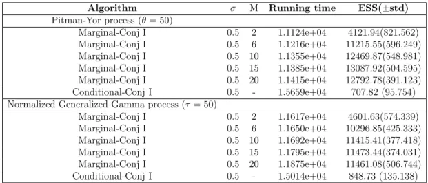
Pitman-Yor process (θ“50) Marginal-Conj I 0.5 2 1.1124e+04 4121.94(821.562) Marginal-Conj I 0.5 6 1.1216e+04 11215.55(596.249) Marginal-Conj I 0.5 10 1.1355e+04 12469.87(548.981) Marginal-Conj I 0.5 15 1.1385e+04 13087.92(504.595) Marginal-Conj I 0.5 20 1.1415e+04 12792.78(391.123) Conditional-Conj I 0.5 - 1.5659e+04 707.82 (95.754)
Normalized Generalized Gamma process (τ “50)
Marginal-Conj I 0.5 2 1.1617e+04 4601.63(574.339) Marginal-Conj I 0.5 6 1.1650e+04 10296.85(425.333) Marginal-Conj I 0.5 10 1.1692e+04 11415.41(377.418) Marginal-Conj I 0.5 15 1.1795e+04 11473.44(374.031) Marginal-Conj I 0.5 20 1.1875e+04 11461.08(506.744) Conditional-Conj I 0.5 - 1.5014e+04 848.73 (135.138)
Table 2: Running times in seconds and number of cluster’s ESS averaged over 10 chains. Unidimensional dataset, 50,000 iterations per chain, 20,000 burn in.
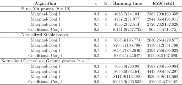
between the auxiliary variables. Finally, in Table 3 we present that different values for σ
can be effectively chosen without modifying the algorithm as opposed to Favaro & Walker (2012), which is only available for σ “0.5.
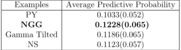
After assessing the algorithm’s performance we used it for inference with a nonparametric mixture model where the top level is a prior from theσ-Stable Poisson-Kingman class. Since any prior in this class can be chosen, one possible criterion for model selection is predictive performance. In Table 4, we reported the average (leave one out) predictive probabilities, see the supplementary material for details. We can see that all priors in this class have similar average predictive probabilities but the NGG slightly outperforms the rest.
In Figure 2, the mode of the posterior distribution is reported, it is around 10 clusters and there are 6 clusters in the coclustering probability matrix. Indeed, a good estimate of the density might include superfluous components having vanishingly small weights as explained
Algorithm σ M Running time ESS(˘std) Pitma-Yor process (θ“10) Marginal-Conj I 0.3 4 4685.7(84.104) 2382.799(169.359) Marginal-Conj I 0.5 4 4757.2(37.077) 2944.065(195.011) Marginal-Conj I 0.7 4 4655.2(52.514) 2726.232(132.828) Conditional-Conj I 0.5 - 10141.6(237.735) 905.444(41.475)
Normalized Stable process
Marginal-Conj I 0.3 4 7658.3(193.773) 2630.264(429.877)
Marginal-Conj I 0.5 4 8203.1(106.798) 3139.412(351.788)
Marginal-Conj I 0.7 4 8095.7(85.2640) 2394.756(295.923)
Conditional-Conj I 0.5 - 10033.1(22.647) 912.382(167.089)
Normalized Generalized Gamma process (τ “1)
Marginal-Conj I 0.3 4 7685.8(208.98) 3587.733(569.984)
Marginal-Conj I 0.5 4 8055.6(93.164) 4443.905(367.297)
Marginal-Conj I 0.7 4 8117.9(113.188) 4936.649(411.568)
Conditional-Conj I 0.5 - 10046.9(206.538) 1000.214(70.148)
Table 3: Running times in seconds and number of cluster’s ESS averaged over 5 chains. Unidimensional dataset, 30,000 iterations per chain, 10,000 burn in.
0 5 10 15 20 25 30 0 0.05 0.1 0.15 0.2 0.25 10 20 30 40 50 60 70 80 10 20 30 40 50 60 70 80 0 0.1 0.2 0.3 0.4 0.5 0.6 0.7 0.8 0.9 1
Figure 2: 210,000 iterations, 10,000 burn in and 20 thinning factor.
in Miller & Harrison (2013). The third plot shows the corresponding density estimate which is consistent under certain conditions as shown in De Blasi et al. (2015).
4.2
Multidimensional experiment
The dataset from de la Mata-Espinosa et al. (2011) consists ofn D-dimensional triacylglyc-eride profiles of different types of oils wheren“120 andD“4000. The observations consist
of profiles of olive, monovarietal vegetable and blends of oils. Within each type there could be several subtypes so we cannot know the number of varieties a priori. We preprocessed the data by applying Principal Component Analysis (PCA) (Jolliffe, 2002) to get the relevant dimensions in it, a useful technique when the signal to noise ratio is small. We used the
Examples Average Predictive Probability
PY 0.1033p0.052q
NGG 0.1228(0.065)
Gamma Tilted 0.1186p0.065q
NS 0.1123p0.057q
Table 4: Unidimensional experiment’s average (leave one out) predictive probabilities. first d“8 principal components which explained 97% of the variance and encoded sufficient
information for the mixture model to recover distinct clusters.
Then a σ-stable Poisson-Kingman mixture of multivariate Normals with unknown co-variance matrix and mean vector was chosen for differenth-tilting functions. A multivariate Normal-Inverse Wishart was chosen as a base measure and the corresponding likelihood F
for the kth cluster:
H0pdµk,dΣkq “Nd ` dµk|µ0, r0Σ´k1 ˘ IWdpdΣk |ν0, S0q Fpdx1, . . . ,dxnk |µk,Σkq “ nk ź i“1 Ndpdxi |µk,Σkq
where X1, . . . , Xnk are the observations currently assigned to cluster k. Nd denotes a d -variate Normal distribution with given mean vector µk and covariance matrix r0Σ´k1, IWd
denotes an inverse Wishart overdˆdpositive definite matrices with given degrees of freedom
and scale matrix. The Inverse Wishart is parameterised as in Gelman et al. (1995). S0 was chosen to be a diagonal matrix with each diagonal element given by the maximum range of the data across all dimensions and degrees of freedom ν“d`3, a weakly informative case.
In Table 5, the average (5-fold) predictive probabilities are reported, see supplementary material for details. Again, we observe that all priors in this class have similar average predictive probabilities. In Figure 3, the mean curve per cluster and the coclustering prob-ability matrix are reported. This mean curve reflects the average triacylglyceride profile per oil type. The coclustering probability matrix was used as an input to an agglomerative clustering algorithm to obtain a hierarchical clustering representation as in Medvedovic & Sivaganesan (2002). In certain contexts, it is useful to think of a hierarchical clustering rather than a flat one, it might be natural to think of superclasses.
In Figure 3, the mean curves per cluster are shown. These were found by thresholding the hierarchy to 8 clusters and ignoring clusters of size one. The first plot corresponds to the
Examples Average Predictive Probability (5 fold)
DP 5.5484e-12 (7.6848e-13)
PY 4.1285e-12 (7.5549e-13)
NGG 9.6266e-12 (3.4035e-12)
Gamma tilted 6.7099e-12(1.5767e-12)
NS 8.3328e-12(9.7106e-13)
Lamperti tilted 5.4251e-12 (1.0538e-12)
Table 5: Multidimensional experiment’s average (5-fold) predictive probabilities. olive oil cluster, it is well represented by the mean curve. The last two plots correspond to data that belongs to olive blends of oil. The third and fourth plots correspond to non-olive monovarietal oil clusters. We could interpret the two clusters as different varieties of vegetable oil since their corresponding mean curves are indeed different. In the dendrogram it is clear that most of the data belongs to 3 large clusters and that 60% of the triacylglycerides are olive oil.
0 0.1 0.2 0.3 0.4 0.5 0.6 0.7 0.8 0.9 1 107111 89 82 59 83 101 91 46 48 87 96 102103 106110 112 99 49 53 80 97 88 81 95 61 98100 51 94 93 22 24 27 31 32 29 37 36 35 30 28 34 33 20 1 2 23 25 26 16 21 54 40 47 75 79 92 50 55105 108109 104 57 58 60 62 63 64 65 66 77 78 52 56 67 3 4 5 6 8 19 9 7 12 11 14113 15 90 10 43 117 42 13 17 18115 41114 39118 45 38 44116 68 70 71 72 73120 74 69 84 85 86 76 119
Dendrogram with Matlab linkage routine
0 500 1000 1500 2000 2500 3000 3500 4000 −5 0 5 10 15 20 25 Cluster size =71 0 500 1000 1500 2000 2500 3000 3500 4000 −2 0 2 4 6 8 10 12 14 16 Cluster size =22 0 500 1000 1500 2000 2500 3000 3500 4000 0 2 4 6 8 10 12 14 16 18 20 Cluster size =6 0 500 1000 1500 2000 2500 3000 3500 4000 −2 0 2 4 6 8 10 12 Cluster size =15 0 500 1000 1500 2000 2500 3000 3500 4000 −1 0 1 2 3 4 5 6 7 8 Cluster size =3
Figure 3: Dendrogram and mean profile per cluster (in red), profiles in each cluster (blue) using a NGG prior.
5
Discussion
A completely random measure completely specifies its total mass but if we allow the total mass to come from a different distribution, we obtain the class of Poisson-Kingman RPMs introduced by Pitman (2003). If we restrict to the σ-stable L´evy measure we obtain the
σ-stable Poisson Kingman class. This class of random probability measures is natural but certain intractabilities have hindered its use. For instance, the intractability associated to the σ-stable density, as noted by Lijoi et al. (2008). The aim of this paper was to review this class of priors and some characterisations which allowed us to build a novel algorithm for posterior simulation that is efficient and easy to use.
Our algorithm is the first sampler of marginal type for mixture models with σ-stable Poisson-Kingman priors. Previously, a conditional sampler has been proposed by Favaro & Walker (2012). One of the advantages of our approach is that the number of auxiliary vari-ables per iteration is smaller than the conditional sampler’s, hence, it has smaller memory and storage requirements. It also has better ESS and running times as shown in our ex-periments. Both conditional and marginal samplers for this class are general purpose: they do not depend on a particular characterisation of a specific Bayesian nonparametric prior as opposed to previous approaches. This makes them very useful and should be added to our Bayesian nonparametrics toolbox. Our approach could be used as a building block in a more complex model using the proposed algorithm. This is an interesting avenue of future research.
6
Acknowledgements
Mar´ıa Lomel´ı thanks the Gatsby Charitable Foundation for generous funding. Stefano Favaro is supported by the European Research Council through StG N-BNP 306406. Yee Whye Teh is supported by the European Research Council under the European Unions Seventh Framework Programme (FP7/2007-2013) ERC grant agreement no. 617411.
References
Aldous, D. 1985. Exchangeability and Related Topics. Pages 1–198 of: ´Ecole d’ ´Et´e de Probabilit´es de Saint-Flour XIII–1983. Springer, Berlin.
Barrios, E., Lijoi, A., Nieto-Barajas, L. E., & Pr¨uenster, I. 2013. Modeling with Normalized Random Measure mixture models. Statistical Science, 28, 283–464.
Bertoin, J. 2006. Random Fragmentation and Coagulation Processes. Cambridge University Press.
Blackwell, D., & McQueen, J. B. 1973. Ferguson distributions via P´olya urn schemes. Annals of Statistics,1, 353–355.
De Blasi, P., Favaro, S., Lijoi, A., Mena, R. H., Pr¨uenster, I., & Ruggiero, M. 2015. Are Gibbs-type priors the most natural generalization of the Dirichlet process? Pages 212–229 of: IEEE Transactions on Pattern Analysis & Machine Intelligence, vol. 37.
de la Mata-Espinosa, P., Bosque-Sendra, J. M., Bro, R., & Cuadros-Rodriguez, L. 2011. Discriminating olive and Non-olive oils using HPLC-CAD and chemometrics. Analytical and Bioanalytical Chemistry,399, 2083–2092.
Devroye, L. 2009. Random variate generation for exponentially and polynomially tilted Stable distributions. ACM Transactions on Modelling and Computer Simulation, 19, 1– 20.
Escobar, M. D. 1994. Estimating normal means with a Dirichlet process prior. Journal of the American Statistical Association, 89, 268–277.
Escobar, M. D., & West, M. 1995. Bayesian density estimation and inference using mixtures. Journal of the American Statistical Association, 90, 577–588.
Ewens, W. J. 1972. The sampling theory of selectively neutral alleles. Theoretical Population Biology, 3, 3 87–112.
Favaro, S., & Teh, Y. W. 2013. MCMC for Normalized Random Measure mixture models. Statistical Science, 28, 335–359.
Favaro, S., & Walker, S. G. 2012. Slice samplingσ-Stable Poisson-Kingman mixture models. Journal of Computational and Graphical Statistics, 22, 830–847.
Favaro, S., Lomeli, M., & Teh, Y. W. 2014. On a class ofσ-stable Poisson-Kingman models and an effective marginalized sampler. Statistics and Computing, 25, 67–78.
Ferguson, T. S. 1973. A Bayesian analysis of some nonparametric problems. Annals of Statistics, 1, 209–230.
Gelman, A., Carlin, J., Stern, H., & Rubin, D. 1995. Bayesian data analysis. Chapman & Hall, London.
Gnedin, A., & Pitman, J. 2006. Exchangeable Gibbs partitions and Stirling triangles.Journal of Mathematical Sciences, 138, 5674–5684.
Griffin, J. E., & Walker, S. G. 2011. Posterior simulation of Normalized Random Measure mixtures. Journal of Computational and Graphical Statistics, 20, 241–259.
Ho, M. W., James, L. F., & Lau, J. W. 2008. Gibbs partitions (EPPFs) derived from a Stable subordinator are Fox H and Meijer G transforms. ArXiv:0708.0619.
Ishwaran, H., & James, L. F. 2001. Gibbs sampling methods for Stick-Breaking priors. Journal of the American Statistical Association, 96, 161–173.
James, L. F. 2002.Poisson process partition calculus with applications to exchangeable models and Bayesian nonparametrics. ArXiv:math/0205093.
James, L. F. 2013.Stick-Breaking PG(α, ψ)-Generalized Gamma processes. ArXiv:1308.6570. James, L. F., Lijoi, A., & Pr¨uenster, I. 2009. Posterior analysis for Normalized Random
Measures with Independent Increments. Scandinavian Journal of Statistics, 36, 76–97. Jolliffe, I.T. 2002. Principal component analysis. 2nd. edn. Springer Verlag, Berlin.
Kalli, M., Griffin, J. E., & Walker, S. G. 2011. Slice sampling mixture models. Statistics and Computing, 21, 93–105.
Kanter, M. 1975. Stable densities under change of scale and total variation inequalities. Annals of Probability,3, 697–707.
Kingman, J. F. C. 1967. Completely Random Measures. Pacific Journal of Mathematics,
21, 59–78.
Kingman, J. F. C. 1975. Random discrete distributions. Journal of the Royal Statistical Society, 37, 1–22.
Kingman, J. F. C. 1978. The representation of partition structures. Journal of the London Mathematical Society, 18, 374–380.
Kingman, J. F. C. 1993. Poisson processes. Oxford University Press.
Laha, R. G., & Rohatgi, V.K. 1979. Probability theory. John Wiley and Sons.
Lijoi, A., Mena, R. H., & Pr¨uenster, I. 2005. Hierarchical mixture modelling with Normalized Inverse-Gaussian priors. Journal of the American Statistical Association,100, 1278–1291. Lijoi, A., Mena, R. H., & Pr¨uenster, I. 2007. Controlling the reinforcement in Bayesian nonparametric mixture models. Journal of the Royal Statistical Society B, 69, 715–740. Lijoi, A., Pr¨unster, I., & Walker, S. G. 2008. Investigating nonparametric priors with Gibbs
structure. Statistica Sinica, 18, 1653 – 1668.
Lo, A.Y. 1984. On a class of Bayesian nonparametric estimates: I. density estimates. Annals of Statistics,12, 351–357.
MacEachern, S. N. 1994. Estimating Normal means with a conjugate Style Dirichlet process prior. Communications in Statistics: Simulation and Computation, 23, 727–741.
Medvedovic, M., & Sivaganesan, S. 2002. Bayesian infinite mixture model based clustering of gene expression profiles. Bioinformatics, 18, 1194–1206.
Miller, J. W., & Harrison, T. M. 2013. A simple example of Dirichlet process mixture inconsistency for the number of components. In: Neural Information Processing Systems. Neal, R. M. 2000. Markov chain sampling methods for Dirichlet process mixture models.
Journal of Computational and Graphical Statistics, 9, 249–265. Neal, R. M. 2003. Slice sampling. Annals of Statistics, 31, 705–767.
Nieto-Barajas, L. E., Pruenster, I., & Walker, S. G. 2004. Normalized Random Measures driven by increasing additive processes. Annals of Statistics, 32, 2343–2360.
Papaspiliopoulos, O., & Roberts, G. O. 2008. Retrospective Markov chain Monte Carlo methods for Dirichlet process hierarchical models. Biometrika,95, 169–186.
Perman, M., Pitman, J., & Yor, M. 1992. Size-biased sampling of Poisson point processes and excursions. Probability Theory and Related Fields,92, 21–39.
Pitman, J. 2003. Poisson-Kingman partitions.Pages 1–34 of: Goldstein, D. R. (ed),Statistics and Science: a Festschrift for Terry Speed. Institute of Mathematical Statistics.
Pitman, J. 2006. Combinatorial Stochastic Processes. Lecture Notes in Mathematics. Springer-Verlag, Berlin.
Pitman, J., & Yor, M. 1997. The two parameter Poisson-Dirichlet distribution derived from a Stable subordinator. Annals of Probability,25, 855–900.
Regazzini, E., Lijoi, A., & Pr¨uenster, I. 2003. Distributional results for means of random measures with independent increments. Annals of Statistics, 31, 560–585.
Roeder, K. 1990. Density estimation with confidence sets exemplified by super-clusters and voids in the galaxies. Journal of the American Statistical Association, 85, 617–624. Tanner, M., & Wong, W. 1987. The calculation of posterior distributions by data
Walker, S. G. 2007. Sampling the Dirichlet mixture model with slices. Communications in Statistics - Simulation and Computation, 36, 45–54.
Wuertz, A., Maechler, M., & Rmetrics core team members. 2013. stabledist. CRAN R Package Documentation.
Zolotarev, V. M. 1966. On the representation of Stable laws by integrals. Selected Transla-tions Math Statist. and Probability,6, 84–88.
A
Matlab Code
Matlabcode Marginalsampler: The folder contains Matlab files with code to perform
posterior inference as described in the article for a unidimensional and multidimensional datasets. The folder also contains all datasets used as examples in the articles and routines for creating plots. (.zip file)
Galaxy data set: Data set from Roeder (1990) used in the unidimensional illustration in
Section 6.1. (.txt file)
Olive oil data set: Data set de la Mata-Espinosa et al. (2011) used in the
B
Additional pseudocode
Algorithm 3SliceSampler(xj, f, E, L)
N1 “N2 “0
Sampley„Ur0, fpxjqs Źf can be an unnormalized density
Samplel „Up0, Lq Ź Lis the chosen length of the interval pa, bq
Set a“xj´l, b “xj ´l`L Ź xj is the previously accepted point
while fpaq ă y_fpbq ă y do ŹSamples xj`1 uniformly from the set fr´1sry,8q
if fpaq ăy then
a“a´E ŹE is the chosen size to enlarge the initial interval
N1 “N1`1 end if if fpbq ă y then b “b`E N2 “N2`1 end if L“b´a Samplel „Up0, Lq Set a“xj ´l, b“xj´l`L end while Set c“xj ´l´N1L,d“xj ´l`N2L Samplew„Upc, dq while fpwq ăy do if wăxj ăb then w„Upw, dq else w„Upc, wq end if end while Returnxj`1 “w Algorithm 4CoClusteringpCq
for m“1ÑM, i“1Ñn, j“1Ñn do Ź M is the number of MCMC iterations
if cm,i ““cm,j then Ź n is the number of data points
Ai,j,m “1 Ź A is a nˆnˆM array else Ai,j,m “0 end if end for P “SumpA,3q{M return
C
Average leave-one-out and 5-fold
predictiverobabil-ities
The posterior predictive density for Xn`1 given X, P and Y“ tY1˚, . . . , Yk˚uis
fσrXn`1 P dx|R, W,X,Y˚s “η0pn`1, σ, k, w, rq ż fpxn`1 |yqppyqdy `η1pn`1, kq k ÿ j“1 pnj´σqf ` xn`1 |yj˚ ˘ where η0pn`1, σ, k, w, rq “ e ´wp1´σqr´σ Γpn`1´σpk`1qq η1pσ, kq “ 1 Γpn`1´σkq
The corresponding empirical estimator, where M is the size of the chain after burn in, is given by: ˆ fσrXn`1 P dx|R, W,X,Y˚s “ 1 M « M ÿ m“1 η0pn`1, σ, km, wm, rmq ż fpxn`1 |yqppyqdy ff ` « η1pn`1, kmq km ÿ j“1 pnj,m´σqf ` xn`1 |y˚j,m ˘ ff
To obtain the average leave-one-out predictive probability we do the following:
1. Fori“1, . . . , n, remove theith observation from the dataset and run the MCMC with
the remaining data points.
2. At each MCMC iteration evaluate the predictive probability of the ith datapoint . 3. Average over theM MCMC iterations to get the average predictive probability for the
ith observation.
After we do this for all observations we take the average of their corresponding predictive probabilities to obtain the average leave one out predictive probability reported in Table 2. To obtain the average 5-fold predictive probability we do the following:
1. For j “ 1, . . . ,5 Randomly split the dataset into training data (4/5) and test data
(1/5) (making sure each observation belongs to the test data only once, in other words, sample without replacement). .
2. At each MCMC iteration evaluate the predictive probability of each test data point and take the average.
3. Average over theM MCMC iterations to get the average predictive probability for the
jth batch of test data.
After we do this for all test data batches we take the average of their corresponding predictive probabilities to obtain the average 5-fold predictive probability reported in Table 3.
D
Examples of EPPFs obtained from Proposition 1
Example 1 (James et al. (2009)). The EPPF of the exchangeable partition Π induced by
NRMpρ, H0q is given by: Pρ,H0pΠn “ pckqkPrKsq “ ż R` un´1 Γpnqe ´ψρpuq du K ź k“1 κρp|ck|, uq where ψρpuq “ ´log ż R` e´utf ρptqdt“ ż R` p1´e´usqρpdsq κρpm, uq “ ż R` vme´uvρ pdvq.
Example 1 can be obtained from Proposition 1 by introducing a disintegration
T´n “ ż R` un´1e´uT Γpnq du,
performing a change of variable S “T ´řKk“1Vk, and marginalizing out S and pVkqkPrKs.
Example 2. The EPPF of the exchangeable partition Π induced by NGGpσ, τq is given by:
Pρ,H0pΠn “ pckqkPrKsq “ ż R` un´1 Γpnqe ´ψρpuqdu K ź k“1 κρp|ck|, uq
where ψρpuq “ ´log ż R` e´utf ρptqdt“ ż R` p1´e´usqρpdsq “ ż R` p1´e´usq a Γp1´σqs ´σ´1e ´τ sds κρpm, uq “ ż R` vme´uvρ pdvq “ a Γp1´σq Γpm´σq pu`τqm´σ.
Example 2 can be obtained if we plug in the NGG’s L´evy measure in Example 1.
Example 3. The EPPF of the exchangeable partition Π induced by PYpθ, σq is given by:
P`Πn“ pckqkPrKs ˘ “σKΓpθq Γpσθq ż R` rθ`Kσ´1exp p´rσq Γpθ`nq K ź k“1 Γp|ck| ´σq Γp1´σq “σKΓpθq Γpσθq Γpσθ `Kq Γpθ`nq K ź k“1 Γp|ck| ´σq Γp1´σq .
The EPPF can be obtained from Proposition 1 by introducing a disintegration
T´pn`θq “ ż R` rn`θ´1e´rT Γpn`θq dr,
performing a change of variables S “ T ´řKk“1Vk, W “ Rσ and marginalizing out S and pVkqkPrKs.
Example 4. The EPPF of the exchangeable partition Π induced by the DPpθq with
concen-tration parameter θ is given by:
P`Πn“ pckqkPrKs ˘ “ ż8 0 ż VK t´nf ρpt´řKk“1vkqdt K ź k“1 v|ck| k ρpdvkq “ θ KΓ pθq Γpn`θq K ź k“1 Γp|ck|q where ρpxq “ θx´1expp´xq fρpxq “ 1 Γpθqx θ´1exp p´xq.
are the L´evy measure of the Gamma Process and the corresponding density function, respec-tively.
Example 4 can be obtained from Proposition 1 by performing a change of variables
Pk “Vk{T for k“1, . . . , K´1, and marginalizing out T and pPkqkPrKs.
E
Proof of Proposition in Perman
et al.
(1992)
Proposition (Perman et al. (1992)). The sequence of surplus masses pSkqkě0 forms a
Markov chain, with initial distribution and transition kernels:
Pρ,H0pS0 P ds0q “ fρps0qds0 Pρ,H0pSk Pdsk|S1 Pds1, . . . , Sk´1 Pdsk´1q “ Pρ,H0pSkPdsk|Sk´1 Pdsk´1q “ psk´sk´1qρpdpsk´sk´1qq sk´1 fρpskq fρpsk´1q .
The proposition can be proven by induction, with each step being an application of the Palm formula (Kingman (1993)) for Poisson processes, similar to the proof of Proposition 2.4 in Bertoin (2006), as follows:
Proof. Induction over k, where k is the number of size biased picks. Let µ “
ř8
k“1ωkδxk be an homogeneous completely random measure.
1. Case k = 1. A size biased sample can be obtained from it in the following way: we
first pick the kth atom with probability ωk
T where T “
ř8
k“1ωk, the kth surplus is
Sk “ T ´
řk
j“1Wj and set W1˚ “ ωk. We are interested in the following conditional
expectation:
EpW1˚ P dω |T P rt, t`sq “ EpW
˚
1 Pdω, T P rt, t`sq
EpT P rt, t`sq (10)
since we can formally define the conditional probability of interest as a weak limit of the conditional expectations indexed by. Furthermore, in this proof it is only done for a simple function of the form δW pdωq but it can be easily extended for a measurable
function f. We can proceed in the following way: if we consider a general simple function, then a non-negative measurable function as a limit of such simple functions and then decompose a measurable functionf in its negative an positive parts (see Laha & Rohatgi (1979)). If we draw from the random measure
PpW1˚ Pdω, T Pdt|µq “ 8 ÿ k“1 ωk T δωkpdωqδTpdtq and then average over it we obtain the numerator in (10):
EpW1˚ Pdω, T P rt, t`sq “E ˜ 8 ÿ k“1 ωk T δωkpdωq, T P rt, t`sq ¸ “ ż ρpyqyδypdwqE`py`Tq´1, y`T P rt, t`s˘ Ñ tρpdωqωfρpt´ωq as Ñ0`
For the third equality, we use Palm’s Formula where GpM, fq “ T1δypdωqIrt,t`spTqand
for the fourth
E`py`Tq´1, y`T P rt, t`s˘“ ż rt´y,t´y`s py`zq´1fρpzqdz ÝÑfρpt´yq t as Ñ0`.
Again, we use the fact that
lim Ñ0` 1 ż rx,x`s ppzqdz “ ż δzpxqppzqdz “ppxq
to obtain the denominator and hence
EpW1˚P dω |T P rt, t`sq ÝÑ ωρpdωqfρpt´ωq
tfρptq as Ñ0`.
2. Suppose the statement holds true for k ą1, i.e.
E`Wk˚ Pdω |T P rt, t`s, Wj˚ Pdωj@j P rk´1s ˘ “ E ˜ W˚ k P dω |T ´ k´1 ÿ j“1 Wj P « t´ k´1 ÿ dωj, t´ k´1 ÿ dωj ` ff¸ ωfρpt´řkj“1ωjq pt´řkj“´11ωjqfρpt´řkj“´11ωjq ρpdωq as Ñ0`.
3. Case k`1. E`Wk˚`1 P dω |T P rt, t`s, Wj˚ Pdωj@j P rks ˘ “ E`Wk˚`1 Pdω, Wj˚ Pdωj,@j P rks, T P rt, t`s ˘ E`Wj˚ Pdωj,@j P rks, T P rt, t`s ˘ .
The denominator is given by the induction hypothesis (IH) so it’s enough to prove this for the numerator:
E`Wk˚`1 Pdω, Wj˚ Pdωj,@j P rks, T P rt, t`s ˘ “ E ˜ 8 ÿ k“1 ωk T δωkpdωjq,@j P rk`1s, T P rt, t`sq ¸ IH “ ż ρpyqyδypdwk`1qE ˜ py`T ´ k ÿ j“1 Wjq´1, y`T ´ k ÿ j“1 Wj P « t´ k ÿ j“1 ωj, t´ k ÿ j“1 ωj` ff¸ Ñ pt´řkj“1ωjq ρpdωqωfρpt´ k`1 ÿ j“1 ωjq as Ñ0`
Where, again, we use the IH in the second equality. Specifically, the fact the sequence of the firstk surpluses masses has the Markov property so it is enough to condition on the last surplus mass. Finally, we obtain:
E`Wk˚`1 Pdω|T P rt, t`s, Wj˚ Pdωj@j P rks ˘ “ ωfρpt´řkj“`11ωjq pt´řkj“1ωjqfρpt´ řk j“1ωjq ρpdωq as Ñ0`.