Distributional regression for demand forecasting in e-grocery

Faculty of Business Administration and Economics

Working Papers in Economics and Management

No. 09-2018

December 2018

Distributional regression for demand forecasting in e-grocery

Matthias Ulrich

Hermann Jahnke

Roland Langrock

Robert Pesch

Distributional regression for demand forecasting

in e-grocery

Matthias Ulrich

, Hermann Jahnke

, Roland Langrock

,

Robert Pesch

, Robin Senge

Abstract

E-grocery offers customers an alternative to traditional brick-and-mortar grocery retailing. Customers select e-grocery for convenience, making use of the home delivery at a selected time slot. In contrast to brick-and-mortar retailing, in e-grocery on-stock information for stock keeping units (SKUs) becomes transparent to the customer before substantial shopping effort has been invested, thus reducing the personal cost of switching to another supplier. As a consequence, compared to brick-and-mortar retailing, on-stock availability of SKUs has a strong impact on the customer’s order decision, resulting in higher strategic service level targets for the e-grocery retailer. To account for these high service level targets, we propose a suitable model for accurately predicting the extreme right tail of the demand distribution, rather than providing point forecasts of its mean. Specifically, we propose the application of distributional regression methods — so-called Generalised Additive Models for Location, Scale and Shape (GAMLSS) — to arrive at the cost-minimising solution according to the newsvendor model. As benchmark models we consider linear regression, quantile regression, and some popular methods from machine learning. The models are evaluated in a case study, where we compare their out-of-sample predictive performance with regard to the service level selected by the e-grocery retailer considered.

Keywords: Forecasting, Inventory, E-commerce, Retailing

1_{Department of Business Administration and Economics, Bielefeld University}

Universit¨atsstraße 25, 33615 Bielefeld, Germany. Email: [email protected]

1

Introduction

In retailing, inventory exceeding or falling short of customer demand generally causes monetary consequences for the retailer. Stock out situations result in term underage costs due to missed sales, whereas excess inventory generates short-term overage costs due to spoilage and operational inefficiencies. However, due to high opportunity costs in retail practice, a service level selected exclusively based on short-term costs may not be profitable. Instead, long-run strategic objectives such as customer loyalty and market growth based on customer satisfaction usually have the most substantial impact on the service level decision (Anderson et al., 2006).

Within the fast-expanding electronic grocery (e-grocery) market, which provides an alternative to traditional brick-and-mortar grocery retailing, the service level is particularly relevant for inventory management. In e-grocery, customers order groceries online and the retailer delivers the purchase to the household or company. Customers use e-grocery for convenience, making use of home delivery at a selected time so that no visit to a brick-and-mortar-store is required. However, if customers are unsatisfied with on-stock availability, then there is a particularly high risk that they cancel the online shopping process, and perhaps even refrain from ordering online in the future. This results from the fact that the convenience of online shopping is reduced once customers need to place a second order or visit a brick-and-mortar store to buy products affected by stock-outs. For perishable SKUs such as fruits, vegetables and meat, customers are particularly restricted with respect to potential substitutes, which further increases the risk of an order cancellation. On-stock availability can hence be expected to be of crucial importance regarding the customers’ order decision. As a consequence, e-grocery retailers operate with very high strategic service level targets, e.g. 97–99% in the case of the retailer considered in our case study, which is in line with service level targets of other international e-grocery retailers, such as Ocado with 98.8% (Ocado Group, 2015). The business problem under consideration in this paper requires customer demand forecasts for each stock keeping unit (SKU) in each local fulfilment centre (FC) for each demand period, which is the lowest hierarchical level in retail demand forecasting. At this level of detail, many different characteristics may affect the underlying demand, rendering demand forecasting very challenging (Fildes et al.,

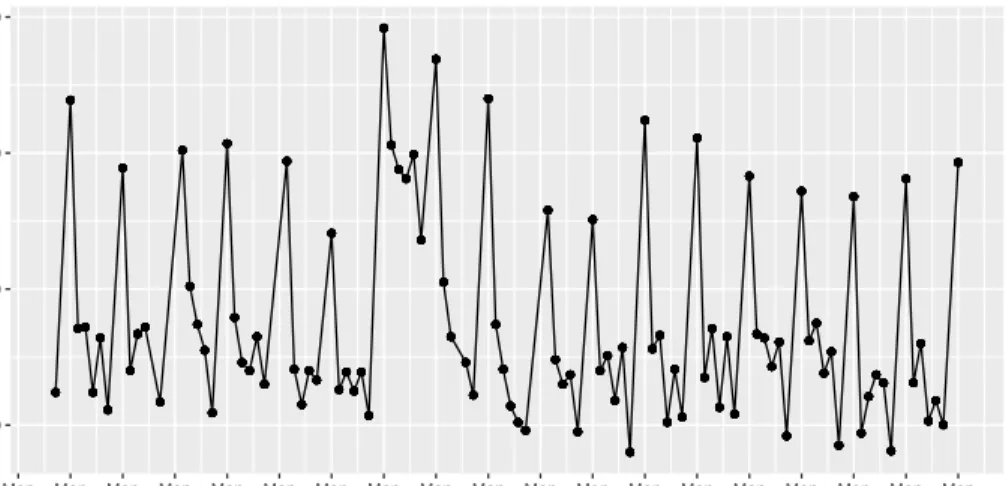
2018). Figure 1 illustrates a small subset of the data considered in our case study, namely customer demand for the SKU grapes in the months April to July 2017. Here one observation equals one demand periodt, i.e. one day of delivery. We find that demand is highly variable, but with recurring peaks on Mondays. These peaks are due to the increased proportion of business-to-business transactions in e-grocery relative to brick-and-mortar retailing. Businesses typically make use of the grocery delivery on Mondays to supply their employees or guests with fruits, coffee and correlated SKUs such as milk.

● ● ● ● ● ● ● ● ● ● ● ● ● ● ● ● ● ● ● ● ● ● ● ● ● ● ● ● ● ● ●● ● ● ● ● ● ● ● ● ● ● ● ● ● ● ● ● ● ● ● ● ●● ● ● ● ● ● ● ● ● ● ● ● ● ● ● ● ● ● ● ● ● ● ● ● ● ●● ● ● ● ● ● ●● ● ● ● ● ● ● ● ● ● ● ● ● ● ● ● ● ● ● ● ● ● ● ● ● ● ● ● ● ● ● ● ● ● ● ● ● ● ● ● ● ● ● ●● ● ● ● ● ● ● ● ● ● ● ● ● ● ● ● ● ● ● ● ● ●● ● ● ● ● ● ● ● ● ● ● ● ● ● ● ● ● ● ● ● ● ● ● ● ● ●● ● ● ● ● ● ●● ● ● ● ● ● ● ● ● ● ● ● ● ● ● ● ● ● ● ● ● ● ● ● ● ● ● ● ● ● ● ● ● ● ● ● ● ● ● ● ● ● ● ●● ● ● ● ● ● ● ● ● ● ● ● ● ● ● ● ● ● ● ● ● ●● ● ● ● ● ● ● ● ● ● ● ● ● ● ● ● ● ● ● ● ● ● ● ● ● ●● ● ● ● ● ● ●● ● ● ● ● ● ● ● ● ● ● ● ● ● ● ● ● ● ● ● ● ● ● ● ● ● ● ● ● ● ● ● ● ● ● ● ● ● ● ● ● ● ● ●● ● ● ● ● ● ● ● ● ● ● ● ● ● ● ● ● ● ● ● ● ●● ● ● ● ● ● ● ● ● ● ● ● ● ● ● ● ● ● ● ● ● ● ● ● ● ●● ● ● ● ● ● ●● ● ● ● ● ● ● ● ● ● ● ● ● ● ● ● ● ● ● ● ● ● ● ● ● ● ● ● ● ● ● ● ● ● ● ● ● ● ● ● ● ● ● ●● ● ● ● ● ● ● ● ● ● ● ● ● ● ● ● ● ● ● ● ● ●● ● ● ● ● ● ● ● ● ● ● ● ● ● ● ● ● ● ● ● ● ● ● ● ● ●● ● ● ● ● ● ●● ● ● ● ● ● ● ● ● ● ● ● ● ● ● ● ● ● ● ● ● ● ● ● ● ● ● ● ● ● ● ● ● ● ● ● ● ● ● ● ● ● ● ●● ● ● ● ● ● ● ● ● ● ● ● ● ● ● ● ● ● ● ● ● ●● ● ● ● ● ● ● ● ● ● ● ● ● ● ● ● ● ● ● ● ● ● ● ● ● ●● ● ● ● ● ● ●● ● ● ● ● ● ● ● ● ● ● ● ● ● ● ● ● ● ● ● ● ● ● ● ● ● ● ● ● ● ● ● ● ● ● ● ● ● ● ● ● ● ● ●● ● ● ● ● ● ● ● ● ● ● ● ● ● ● ● ● ● ● ● ● ●● ● ● ● ● ● ● ● ● ● ● ● ● ● ● ● ● ● ● ● ● ● ● ● ● ●● ● ● ● ● ● ●● ● ● ● ● ● ● ● ● ● ● ● ● ● ● ● ● ● ● ● ● ● ● ● ● ● ● ● ● ● ● ● ● ● ● ● ● ● ● ● ● ● ● ●● ● ● ● ● ● ● ● ● ● ● ● ● ● ● ● ● ● ● ● ● ●● ● ● ● ● ● ● ● ● ● ● ● ● ● ● ● ● ● ● ● ● ● ● ● ● ●● ● ● ● ● ● ●● ● ● ● ● ● ● ● ● ● ● ● ● ● ● ● ● ● ● ● ● ● ● ● ● ● ● ● ● ● ● ● ● ● ● ● ● ● ● ● ● ● ● ●● ● ● ● ● ● ● ● ● ● ● ● ● ● ● ● ● ● ● ● ● ●● ● ● ● ● ● ● ● ● ● ● ● ● ● ● ● ● ● ● ● ● ● ● ● ● ●● ● ● ● ● ● ●● ● ● ● ● ● ● ● ● ● ● ● ● ● ● ● ● ● ● ● ● ● ● ● ● ● ● ● ● ● ● ● ● ● ● ● ● ● ● ● ● ● ● ●● ● ● ● ● ● ● ● ● ● ● ● ● ● ● ● ● ● ● ● ● ●● ● ● ● ● ● ● ● ● ● ● ● ● ● ● ● ● ● ● ● ● ● ● ● ● ●● ● ● ● ● ● ●● ● ● ● ● ● ● ● ● ● ● ● ● ● ● ● ● ● ● ● ● ● ● ● ● ● ● ● ● ● ● ● ● ● ● ● ● ● ● ● ● ● ● ●● ● ● ● ● ● ● ● ● ● ● ● ● ● ● ● ● ● ● ● ● ●● ● ● ● ● ● ● ● ● ● ● ● ● ● ● ● ● ● ● ● ● ● ● ● ● ●● ● ● ● ● ● ●● ● ● ● ● ● ● ● ● ● ● ● ● ● ● ● ● ● ● ● ● ● ● ● ● ● ● ● ● ● ● ● ● ● ● ● ● ● ● ● ● ● ● ●● ● ● ● ● ● ● ● ● ● ● ● ● ● ● ● ● ● ● ● ● ●● ● ● ● ● ● ● ● ● ● ● ● ● ● ● ● ● ● ● ● ● ● ● ● ● ●● ● ● ● ● ● ●● ● ● ● ● ● ● ● ● ● ● ● ● ● ● ● ● ● ● ● ● ● ● ● ● ● ● ● ● ● ● ● ● ● ● ● ● ● ● ● ● ● ● ●● ● ● ● ● ● ● ● ● ● ● ● ● ● ● ● ● ● ● ● ● ●● ● ● ● ● ● ● ● ● ● ● ● ● ● ● ● ● ● ● ● ● ● ● ● ● ●● ● ● ● ● ● ●● ● ● ● ● ● ● ● ● ● ● ● ● ● ● ● ● ● ● ● ● ● ● ● ● ● ● ● ● ● ● ● ● ● ● ● ● ● ● ● ● ● ● ●● ● ● ● ● ● ● ● ● ● ● ● ● ● ● ● ● ● ● ● ● ●● ● ● ● ● ● ● ● ● ● ● ● ● ● ● ● ● ● ● ● ● ● ● ● ● ●● ● ● ● ● ● ●● ● ● ● ● ● ● ● ● ● ● ● ● 100 200 300 400

Mon Mon Mon Mon Mon Mon Mon Mon Mon Mon Mon Mon Mon Mon Mon Mon Mon Mon Mon realised demand for SKU grapes in the months April to July 2017

realised demand in units

Figure 1: Realised demand for the SKU grapes in units (package of 500 gr), with highly variable demand but recurring peaks on Monday.

In traditional brick-and-mortar retailing, information on customer demand typi-cally results from point-of-sale data. These data often do not reveal the true demand preferences due to stock-outs affecting the individual purchase, and are therefore effectively censored. This distortion in customer demand for one SKU has an impact also on demand data for correlated SKUs that are not purchased although available (e.g. mozzarella, if tomatoes are out) and demand data of selected substitutes that generate sales without original demand. Predicted demand of an SKU that was sub-ject to stock-outs in the past and of corresponding SKUs affected by the correlation effect will therefore be potentially too low, whereas predicted future demand of selected substitutes will potentially be too high (Anupindi et al., 1998). In contrast

to traditional retailing, the online customer order process of the e-grocery retailer considered in our case study allows for the monitoring of customer preferences

beforestock-out information becomes available to the buyer and, therefore, yields uncensored demand data. Stock-outs do affect sales data but not the demand data re-vealed by the customer’s online search behaviour, which precedes the final purchase decision. Tracing the customer’s search behaviour hence yields uncensored demand data. Moreover, in e-grocery a customer selects a future delivery time slot with up to fourteen days in advance to make sure he or she is able to receive the order at home. Depending on the delivery time slot selected by the customer, the e-grocery retailer can include the customer demand information in the replenishment order. Thus, the e-grocery retailer does not have to hold all inventory requested at the time of the customer order, but may replenish the SKU before the order needs to be dispatched.

Given the wide range of demand patterns of SKUs on offer (e.g. fast-moving or slow-moving SKUs with regular or irregular demand), it seems unlikely that a simple statistical modelling framework such as linear regression will be suitable across the range of SKUs. For SKUs in grocery retailing, most results reported in the literature do indeed identify potential improvements by using nonlinear models (Ali et al., 2009 and Lang et al., 2015). In fact, since we are interested in very high service levels, and hence need to be able to accurately predict the extreme right tail of the forecast distribution, any regression method that focuses on themeanwould not seem to be an intuitive choice. Quantile regression, where specific quantiles of the response variable (here: demand) are linked to covariates, constitutes a much more obvious alternative given the high service level targets (Manning et al., 1995 and Kneib, 2013). However, using quantile regression to predict the extreme (right) tail of the response distribution can be problematic, since the corresponding parameter estimators can be highly imprecise due to data scarcity in the extreme tails (Hohberg et al., 2018). In recent years, distributional regression methods, which allow flexible modelling of covariate effects onanyof the distributional parameters (including mean and variance), have rapidly gained popularity as versatile statistical modelling tools that allow to consider various aspects of the response distribution (e.g. Mayr et al., 2012 and Klein et al., 2015). In contrast to quantile regression methods, which are nonparametric, distributional regression methods are parametric. Sachs & Minner (2014) compared parametric and nonparametric modelling approaches for

estimating different censoring levels using data from a large European retail chain. They showed that their nonparametric model copes well with highly censored data, but also pointed out that the parametric alternatives performed best if there is little censoring in the demand.

Considering data from a leading German omni-channel retailer, here we aim to exploit the associated new types of data in e-grocery that are not available in traditional brick-and-mortar retailing, i.e. uncensored customer demand and partly known future demand data, to model the entire demand distribution. Specifically, we propose the application of Generalized Additive Models for Location, Scale and Shape (GAMLSS) for building flexible distributional regression models to forecast demand in e-grocery retailing. In particular, these models consider no only the mean of future demand, but also its variance and potentially even the shape as functions of covariates. In addition, the GAMLSS class allows a flexible choice of the distributional family assumed for the response variable, i.e. for demand. Thus, GAMLSS allows us to tailor the regression model to whatever complex pattern we find, while likely being more robust than quantile regression methods.

We compare the performance of GAMLSS with basic (parametric) linear regres-sion and (nonparametric) quantile regresregres-sion, evaluating the models by comparing their out-of-sample forecasting error at the selected service level with the corre-sponding cost values for underage and overage. Given the increasing popularity of machine learning methods (see, e.g., Carbonneau et al., 2008, Ferreira et al., 2016), we also include parametric random forests (Breiman, 2001) and nonpara-metric quantile regression forests (Meinshausen, 2006) as benchmarks. For the SKUs considered in our case study, we find that models from the GAMLSS class tend to outperform the benchmark models, with the (cost-) optimal distributional assumption to be made for the response variable varying across SKUs.

2

Problem statement and motivation

2.1 Demand forecasting and the newsvendor problem

The e-grocery retailer considered in our case study offers a significant number of perishable SKUs in the product category fruits, vegetables and meat. Internal quality

requirements of the retailer restrict the shelf life of these SKUs to one demand period. In addition, SKUs with stock-outs in the demand period are not delivered to the customer at a later demand period. We hence assume that the customer demand and the sales period are identical for the SKUs analysed in the case study. As a result, excess inventory cannot be sold in the following demand period and thus generates spoilage.

To capture the asymmetric economic impact of absolute forecasting errors for each demand periodt, we introduce the total costCt resulting from any potential

mismatch between inventory level and realised demand. In demand periodt, each excess unit of inventory generates a cost ofh, while each unit that we fall short of customer demand generates a cost ofb. Furthermore, we useDt to denote the

stochastic customer demand. We then aim at minimising the expected total cost,

E[Ct(qt)] =hE(qt−Dt)++bE(Dt−qt)+, (1)

with respect to the inventory level at the beginning of the demand period,qt. The

optimalqt defines the corresponding replenishment order quantity of the retailer for

periodt.

For single and independent demand periods with stochastic customer demand, the newsvendor problem provides the solution to the optimisation problem above. The newsvendor problem is one of the classical applications in the literature on inventory management for problems with characteristics as given here (Zipkin, 2000). The optimal inventory level is obtained as

q_t∗=argmin

qt

E[Ct(qt)] =Ft−1 b/(b+h)

, (2)

whereFt is the (true) cumulative distribution function of the demand distribution

in periodt, and b/(b+h) is the optimal demand quantile given b and h. The ratiob/(b+h) can also be interpreted as the inventory service level selected by the retailer. In practice, the optimal solution to the newsvendor problem given in (2) is not available since the cumulative distribution functionFt describing the

stochastic demand is unknown. However, we can use data collected before timetto statistically model realised demand as a function of features (e.g. known demand at

the time of the replenishment order), and subsequently predict demandqt using the

estimated distribution function ˆFt obtained under the model. Thus, we are looking

for a suitable distributional regression model, rather than point forecasts only, to minimise the costs of the e-grocery retailer.

2.2 Demand forecasting in the existing literature

In the retailing context, the newsvendor problem is one of the most intensively studied inventory management problems in literature; see Khouja (1999) and Qin et al. (2011) for extensive literature reviews with different applications for individual problem characteristics.

Early papers from this research area assume that the demand distribution is completely known (Arrow et al., 1951). Scarf et al. (1959) relaxed this assumption by assuming that only the mean and the standard deviation are known. Since those early contributions, various parametric (e.g. Nahmias, 1994, Agrawal & Smith, 1996) and nonparametric (e.g. Lau & Lau, 1996, Godfrey & Powell, 2001) approaches have been proposed to identify the cost-optimal inventory levelqfor the case where the demand distribution is unknown and hence needs to be estimated or otherwise specified.

Parametric approaches to determine the expected-cost optimal order quantityq

focus on the estimation of the mean by a point prediction and derive the standard deviation from historic demand variations. Based on the expected demand pattern, different distributional assumptions are proposed, e.g. normal (Nahmias, 1994), gamma (Burgin, 1975), Poisson (Conrad, 1976), and negative binomial (Agrawal & Smith, 1996). In retail practice withb>h, the inventory levelqminus the estimated mean is often interpreted as the safety stock to cope with forecasting errors (e.g. Baker et al., 1986).

Linear regression is the most established approach for modelling directed rela-tionships, and as such is also a popular tool for demand point forecasting (see, e.g., Makridakis et al., 1998, and Weisberg, 2005). However, linear regression involves several restrictive assumptions, namely linearity of the predictor, homoscedasticity and, when forecast distributions are of interest, also normality of the response. For at least some of the SKUs on offer, these will be violated, for example if the

distribution of slow-moving SKUs is neither normal nor symmetric (Ramaekers & Janssens, 2008). In those instances, demand forecasts obtained through linear regression may be imprecise.

For point forecasts of the mean, machine learning techniques have rapidly increased in popularity as an alternative to linear regression (see, e.g., Carbonneau et al., 2008, Ferreira et al., 2016). For example, random forests have been successfully applied in the context of load forecasting on the electricity market (Lahouar & Ben Hadj Slama, 2015).

Quantile regression is a natural nonparametric alternative which focusses on forecasting selected quantiles rather than the mean (Koenker & Hallock, 2001, Maciejowska et al., 2016). In particular, within quantile regression we avoid making any distributional assumption for the response. However, a potential problem with using quantile regression methods for e-grocery demand forecasting is that we often see extreme outliers in the realised demand data to which quantile methods may react more strongly than distributional regression models. These outliers are due to the high proportion of business-to-business transactions as discussed above. Meinshausen (2006) proposed quantile regression forests as a competitive alternative to quantile regressions.

2.3 E-grocery business processes

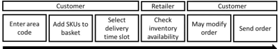
Irrespective of the particular approach taken, we aim to make use of the new types of data in e-grocery that are not available in traditional retailing. To better understand the corresponding data, we first introduce the business processes that generate these new types of data. The complete process of a customer’s order is displayed in Figure 2. Customers first enter the area code, which determines the associated FC with a given assortment. During the shopping process, no inventory information is provided to the customer, such that any desired SKU can simply be added to the basket, without restrictions resulting from its availability status. This allows for the observation of customer preferencesbeforestock-out information is made available. At the customer checkout, an algorithm checks the inventory availability of the requested SKUs for the selected delivery time slot. In case of missing inventory, a suitable substitute is offered to the customer, who can then modify the order.

Figure 2: Customer order process in e-grocery.

The replenishment and fulfilment process of the e-grocery retailer is shown in Figure 3. The national and regional distribution centres supply the FC based on replenishment orders. Operational fulfilment processes include stowing, picking, and the distribution to the customer. It typically takes three days from placing the replenishment order to receiving the goods at the FC. Thus, if the customer orders more than three days in advance to the delivery slot, then known demand can be considered for the replenishment order.

Figure 3: Replenishment and fulfilment process in e-grocery.

2.4 Exploratory analysis of the e-grocery data

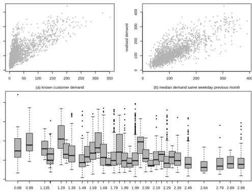
In the following, we explore the e-grocery data available in our case study in order to motivate the choice of the class of GAMLSS. To illustrate some of the key patterns, Figure 4 displays the relationship between selected explanatory variables (features) and the response variable, realised demand, for the SKU grapes from September 2015 to August 2017, for one FC. We find,inter alia, the following patterns:

1. Nonlinearity

replenishment decision time and realised demand.1 Realised demand equals or exceeds known demand for each observation. For relatively low known demand, i.e. below 100 units, the size of additional demand occurring during the replenishment period is relatively high compared to situations where known demand is already high, i.e. above 100 units. This indicates that the functional relationship between realised demand and known demand is nonlinear. ● ● ● ● ● ● ● ● ● ● ● ● ● ● ● ● ● ● ● ● ● ● ● ● ● ● ● ● ● ● ● ●● ● ● ● ● ● ● ● ● ● ● ● ● ● ● ● ● ● ● ● ●● ● ● ● ● ●● ● ● ● ● ● ● ● ● ● ● ● ● ● ● ●● ● ● ● ● ● ● ● ● ● ● ● ● ● ●● ● ● ● ● ● ● ● ● ●● ●● ● ● ● ● ● ● ● ● ● ● ● ● ● ● ● ● ● ● ● ● ● ● ● ● ● ● ● ● ● ● ● ● ● ● ● ● ● ● ● ● ● ● ● ● ● ● ● ● ● ● ● ● ● ● ● ● ● ●● ● ● ● ● ● ● ● ● ● ● ● ● ● ● ● ● ● ● ● ● ● ● ● ●● ● ● ● ● ● ● ● ● ● ● ● ● ● ● ● ● ●● ● ● ● ● ● ● ● ● ● ● ● ● ● ● ● ● ● ● ●● ● ● ● ● ● ● ● ● ● ● ● ● ● ● ● ● ● ● ● ● ● ● ● ● ● ● ● ● ● ● ● ● ● ● ● ● ● ● ● ● ● ● ● ● ● ● ● ● ● ● ● ● ● ● ● ● ● ● ● ● ● ● ● ● ● ● ● ● ● ● ● ● ● ● ● ● ● ● ● ● ● ● ● ● ● ● ● ● ● ● ● ● ● ● ● ● ● ● ● ● ● ● ● ●● ● ● ● ● ● ● ● ● ● ● ● ● ● ● ● ● ● ● ● ●● ● ● ● ● ● ● ● ● ● ● ● ● ● ● ● ● ● ● ● ● ● ● ● ● ● ● ● ● ● ● ● ● ● ● ● ● ● ● ● ● ● ● ● ● ● ● ● ● ● ● ● ● ● ● ● ● ● ● ● ● ● ● ● ● ● ● ● ● ● ● ● ● ● ● ● ● ● ● ● ● ● ● ● ● ● ● ● ● ● ● ● ● ● ● ● ● ● ● ● ● ● ● ● ● ●● ● ● ● ● ● ● ● ● ● ● ● ● ● ● ● ●● ● ● ● ● ● ● ● ● ● ● ● ● ● ● ● ● ● ● ● ● ● ● ● ● ● ● ● ● ● ● ● ● ● ● ● ● ● ● ● ● ● ● ● ● ● ● ● ● ● ● ● ● ● ● ● ● ● ● ● ● ● ● ● ● ● ● ● ● ● ● ● ● ● ●● ● ● ● ● ● ● ● ● ● ● ● ● ● ● ● ● ● ● ● ● ● ● ● ● ● ● ● ● ●● ● ● ● ● ● ● ● ● ● ● ● ● ● ● ● ● ● ● ● ● ● ● ● ● ● ● ● ● ● ● ● ● ● ● ● ● ● ● ● ● ● ● ● ● ●●● ● ● ● ● ● ● ● ● ● ● ● ● ● ● ● ● ● ● ● ● ● ● ● ● ● ● ● ● ● ● ● ● ● ● ● ● ● ● ● ● ● ● ● ● ● ● ● ● ● ● ● ● ● ● ● ● ● ● ● ● ● ● ● ● ● ●● ● ● ● ● ● ● ● ● ● ● ● ● ● ● ● ● ● ● ● ● ● ● ● ● ● ● ● ●● ● ● ● ● ● ● ● ● ● ●● ● ● ● ● ● ● ● ● ● ● ● ● ● ● ● ●● ● ● ● ● ● ● ● ● ● ● ● ● ● ● ● ● ● ● ● ● ● ● ● ● ● ●● ● ● ● ● ● ● ● ● ● ● ● ● ● ● ●● ● ● ● ● ● ● ● ● ● ● ● ● ● ● ● ● ●● ● ● ● ● ● ● ● ●● ● ● ● ● ● ● ● ● ● ● ● ●●● ● ● ● ●● ● ● ● ● ● ● ● ● ● ● ● ● ● ● ● ● ● ● ● ● ● ● ● ● ● ● ● ● ● ● ● ● ● ● ● ● ● ● ● ● ● ● ● ● ● ● ● ● ● ● ● ● ● ● ● ● ● ● ● ● ● ● ● ●● ● ● ● ● ● ● ● ●● ● ● ● ● ● ● ● ● ● ● ● ● ● ● ● ● ● ● ● ● ● ● ● ● ●● ● ● ● ● ● ● ● ● ● ● ● ● ● ● ●● ● ● ● ● ● ● ● ● ● ● ● ● ● ● ● ● ● ● ● ●●● ● ● ● ● ● ● ● ● ● ● ● ● ● ● ● ● ● ● ● ● ● ● ● ● ● ● ● ● ●● ● ● ● ● ● ● ● ● ● ● ● ● ● ● ● ● ● ● ● ● ● ● ● ● ● ● ● ● ● ● ● ● ● ● ● ● ● ● ● ● ● ● ● ● ● ● ● ● ● ● ● ● ● ● ● ●● ● ● ● ● ● ● ● ● ● ● ● ● ●● ● ●● ● ● ● ● ● ● ● ● ● ● ● ●● ● ● ● ● ●●●●● ● ● ● ● ● ● ● ● ● ● ● ● ● ● ● ● ● ● ● ● ● ● ● ● ● ● ● ● ● ● ● ● ● ● ● ● ● ● ● ●● ● ● ● ● ● ● ● ● ● ● ● ● ● ● ● ● ● ● ● ● ● ● ● ● ● ● ● ● ● ● ● ● ● ● ● ● ● ● ● ● ● ● ● ● ● ● ● ● ●● ● ● ● ● ● ● ● ● ● ● ● ● ● ● ● ● ●● ● ● ● ● ● ● ● ● ● ● ● ● ● ● ● ● ● ● ● ● ● ● ● ● ● ● ● ● ● ● ● ● ● ● ● ● ● ● ● ● ● ● ● ● ● ● ● ● ● ● ● ● ● ● ● ● ● ● ● ● ● ● ● ● ● ● ●● ● ● ● ● ● ● ● ● ● ● ● ● ● ● ● ● ● ● ● ● ● ● ● ● ● ● ● ● ● ● ● ● ● ● ● ● ● ● ● ● ● ●● ● ● ● ● ● ● ● ● ● ● ● ● ● ● ● ● ● ● ● ● ● ● ● ● ● ● ● ● ● ● ● ● ● ● ● ● ● ● ● ● ● ● ● ● ● ● ● ● ● ● ● ● ● ● ● ● ● ● ● ● ● ● ● ● ● ● ● ● ● ● ● ● ● ● ● ● ● ● ● ● ● ● ● ● ● ● ● ● ● ● ● ● ● ● ● ● ● ● ● ● ● ● ● ● ● ● ● ● ● ● ●● ● ● ● ● ● ● ● ● ● ● ● ● ● ● ● ● ● ● ● ● ● ● ● ● ● ● ● ● ● ● ● ● ● ● ● ● ● ● ● ● ● ● ● ● ● ● ● ● ● ● ● ● ● ●● ● ● ● ● ● ● ● ● ● ● ● ● ● ● ● ● ● ● ● ● ● ● ● ● ● ● ● ● ● ●● ● ● ● ● ● ● ● ● ● ● ● ● ● ● ● ● ● ● ● ● ● ● ● ● ● ● ● ● ● ● ● ● ●● ● ● ● ● ● ● ● ● ● ● ● ● ● ● ● ● ● ● ● ● ● ● ● ● ● ● ● ● ● ● ● ● ● ● ● ● ● ● ● ● ● ● ● ● ● ● ● ● ● ● ● ● ● ● ● ● ● ● ● ● ● ● ● ● ● ● ● ● ● ● ● ● ● ● ● ● ● ● ● ● ● ● ● ● ● ● ● ● ● ● ● ● ● ● ● ●● ● ● ● ● ● ● ● ● ● ● ● ● ● ● ● ● ● ● ● ● ● ● ● ● ● ● ● ● ● ● ● ● ● ● ● ● ● ● ● ● ● ● ● ● ● ● ● ● ● ● ● ● ● ●● ● ● ● ● ● ● ● ● ● ● ● ● ● ● ● ● ● ● ● ● ● ● ● ● ● ● ● ● ● ● ● ● ● ● ● ● ● ● ● ● ● ● ● ●● ●● ● ● ● ● ● ● ● ● ● ● ● ● ● ● ● ● ● ● ● ● ● ● ● ● ● ● ● ● ● ● ● ● ● ● ● ● ● ● ● ●●● ● ● ● ● ● ● ● ● ● ● ● ● ● ● ● ● ● ● ● ● ● ● ● ● ● ● ● ● ● ● ● ● ● ● ● ● ● ● ● ● ● ● ● ● ● ● ● ● ●● ● ● ● ● ● ● ● ● ● ● ● ● ● ● ● ● ● ● ● ● ● ● ● ● ● ● ● ● ● ● ● ● ●● ● ● ● ● ● ● ● ● ● ● ● ● ● ● ● ● ● ●● ●● ● ●● ● ● ● ● ● ● ● ●● ● ● ● ● ● ● ● ● ● ● ● ● ● ● ● ● ● ● ● ●● ● ● ● ● ● ● ● ● ● ● ● ● ● ● ● ● ● ● ● ● ● ● ● ●● ● ●● ● ● ● ● ● ● ● ● ● ● ● ● ●● ● ● ●● ● ● ● ● ● ● ● ● ● ● ● ● ● ● ● ● ● ● ● ● ● ● ●● ● ● ● ● ● ● ● ● ● ● ● ● ● ● ● ● ● ● ● ● ● ● ● ● ● ● ● ● ● ● ● ● ● ● ● ● ● ● ● ● ● ● ● ● ● ● ● ● ● ● ● ● ●● ● ● ● ● ● ● ● ● ● ● ● ● ● ● ● ● ● ● ● ●● ● ● ●● ● ● ● ● ● ● ● ● ● ● ● ● ● ● ● ● ● ● ● ● ● ● ● ● ● ● ● ● ● ● ● ● ● ● ● ● ● ● ● ● ● ● ● ● ● ● ●● ● ● ● ● ● ● ● ● ● ● ● ● ● ● ● ● ● ● ● ● ● ● ● ● ● ● ● ● ● ● ●● ● ● ● ● ● ● ● ● ● ● ● ● ● ● ●● ● ● ● ● ● ● ● ● ● ● ● ● ● ● ● ● ● ● ●● ● ● ● ● ● ● ● ● ● ● ● ● ● ● ● ● ● ● ● ● ● ● ● ● ● ● ● ● ● ● ● ● ● ● ● ● ● ● ● ● ● ● ● ● ● ● ● ● ● ● ● ● ● ● ● ● ● ● ● ● ● ●● ● ● ● ● ● ● ● ● ● ● ● ● ● ● ● ● ● ● ● ● ● ● ● ● ● ● ● ● ● ● ● ● ● ● ● ● ● ● ● ● ● ● ● ● ● ● ● ● ● ● ● ● ● ● ● ● ● ● ● ● ● ● ● ● ● ● ● ● ● ● ● ● ● ● ● ●● ● ● ● ● ● ● ● ● ● ●● ● ● ● ● ● ● ● ● ● ● ●● ● ● ● ● ● ● ● ● ● ● ● ● ● ● ● ● ● ● ● ● ● ● ● ● ● ● ● ● ● ● ● ● ● ● ● ● ● ● ● ● ● ● ● ● ● ● ● ● ● ● ● ● ● ●● ● ● ● ● ● ● ● ● ● ● ● ● ● ● ● ● ● ● ● ● ● ● ● ● ● ● ● ● ● ● ● ● ● ● ● ● ● ● ● ● ● ● ● ● ● ● ● ● ● ●● ● ● ● ● ● ● ● ● ● ● ● ● ● ● ● ● ● ● ● ● ● ● ● ● ● ● ● ● ● ● ● ● ● ● ● ● ● ● ● ● ● ● ● ● ● ● ● ● ●● ● ● ● ● ●● ● ● ● ● ● ● ● ● ● ● ● ● ● ● ● ● ● ● ● ● ● ● ● ● ● ● ● ● ● ● ● ● ● ● ● ● ●● ● ● ● ● ● ● ● ● ● ● ● ●● ● ● 0 50 100 150 200 250 300 350 0 100 200 300 400

(a) known customer demand

realised demand ● ● ● ● ● ● ● ● ● ● ● ● ● ●● ● ● ● ● ● ● ● ● ● ● ● ● ● ● ● ● ● ● ● ● ● ● ● ● ● ● ● ● ● ● ● ● ● ● ● ● ●●● ● ● ● ● ● ● ● ● ● ● ● ● ● ● ● ● ● ● ● ● ● ● ● ● ● ● ● ● ● ● ● ● ● ● ● ● ● ● ● ● ● ● ● ● ● ● ● ● ● ● ● ● ● ● ● ● ● ● ● ● ● ● ● ● ● ● ● ● ● ● ● ● ● ● ● ● ● ● ● ● ● ● ● ● ● ● ● ● ● ● ● ● ● ● ● ● ● ● ● ● ● ● ● ● ● ● ●● ● ● ● ● ●● ● ● ● ● ● ● ● ● ● ● ● ● ● ● ●● ● ● ● ● ● ● ● ● ● ● ● ● ● ● ● ● ● ● ● ● ● ● ● ● ● ● ● ● ● ● ● ● ● ● ●● ● ● ● ● ● ● ● ● ● ● ● ● ● ● ● ● ● ● ● ● ● ● ● ● ● ● ● ● ● ● ● ● ● ● ● ● ● ● ● ● ● ● ● ● ● ● ● ● ● ● ● ● ● ● ● ● ● ● ● ● ● ● ● ● ● ● ● ● ● ● ● ● ● ● ● ● ● ● ● ● ● ● ● ● ● ● ● ● ● ● ● ● ● ● ● ● ● ● ● ● ● ● ● ● ● ● ● ●●● ● ● ● ● ● ● ● ● ● ● ● ● ● ● ● ● ● ● ● ● ● ● ● ● ● ● ● ● ● ● ● ● ● ● ● ● ● ● ● ● ● ● ● ● ● ● ● ● ● ● ● ● ● ● ● ● ● ● ● ● ● ● ● ● ● ● ● ● ● ● ● ● ● ● ● ● ● ● ● ● ● ● ● ● ● ● ● ● ● ● ● ● ● ● ● ● ● ● ● ● ● ● ● ● ● ● ● ● ● ● ● ● ● ● ● ● ● ● ● ● ● ● ● ● ● ● ● ● ● ● ● ● ● ● ● ● ● ● ● ●● ● ● ● ● ● ● ● ● ● ● ● ● ● ● ● ● ● ● ● ● ● ● ● ● ● ● ● ● ● ● ● ● ● ● ● ● ● ● ● ● ● ● ● ● ● ● ● ● ● ● ● ● ● ● ● ● ● ● ● ● ● ● ● ● ● ● ● ● ● ● ● ● ● ● ● ● ● ● ● ● ● ● ● ● ● ● ● ● ● ● ● ● ● ● ● ● ● ● ● ● ● ● ● ● ● ● ● ● ● ● ● ● ● ● ● ● ● ● ● ● ● ● ● ● ● ● ● ● ● ● ● ● ● ● ● ● ● ● ● ● ● ● ● ● ● ● ● ● ● ● ● ● ● ● ● ● ● ● ● ● ● ● ● ● ● ● ● ● ● ● ● ● ● ● ● ● ● ● ● ● ● ● ● ● ● ● ● ● ● ● ● ● ● ● ● ● ● ● ● ● ● ● ● ● ● ● ● ● ● ● ● ● ● ● ● ● ● ● ● ● ● ● ● ● ● ● ● ● ● ● ● ● ● ● ● ● ● ● ● ● ● ● ● ● ● ● ● ● ● ●● ● ● ● ● ● ● ● ● ● ● ● ● ● ● ● ● ● ● ● ● ● ● ● ● ● ● ● ● ● ● ● ● ● ● ● ● ● ● ● ● ● ● ● ● ● ● ● ● ● ● ● ● ● ●● ● ● ● ● ● ● ● ● ● ● ● ● ● ● ● ● ● ● ● ● ● ● ● ● ● ● ● ● ● ● ● ●● ● ● ●● ● ● ● ● ●● ● ● ● ● ● ● ● ● ● ● ● ● ●● ● ● ● ● ● ● ● ● ● ● ● ● ● ● ● ● ● ● ● ● ● ● ● ● ● ● ● ● ● ● ● ● ● ● ● ● ● ● ● ● ● ● ● ● ● ● ● ● ● ● ● ● ● ● ● ● ● ● ● ● ● ● ● ● ● ● ● ● ● ● ● ● ● ● ● ● ● ● ● ● ● ● ● ● ● ● ● ● ● ● ● ● ● ● ● ● ● ● ● ● ● ● ●● ● ● ● ● ● ● ● ● ● ● ● ● ● ● ● ● ● ● ● ● ● ● ● ● ●● ●● ● ● ● ● ● ● ● ● ●●● ● ● ● ● ● ● ● ● ● ● ● ● ● ● ● ● ● ● ● ● ● ● ● ● ● ● ● ● ●● ● ● ● ● ● ● ● ● ● ● ● ● ● ● ● ● ● ● ● ● ● ● ● ● ● ● ● ● ● ● ● ● ● ● ● ● ● ● ● ● ● ● ● ● ● ● ● ● ● ● ● ● ● ● ● ● ● ● ● ● ● ● ● ● ● ● ● ● ● ●● ● ● ● ● ● ● ● ● ● ● ●● ● ●● ● ● ● ● ● ●● ●●● ● ● ● ● ● ● ● ● ● ● ● ● ● ● ● ● ● ● ● ● ● ● ● ● ● ● ● ● ● ● ● ● ● ● ● ● ● ● ● ● ● ● ● ● ● ● ● ● ● ● ● ● ● ● ● ● ● ● ● ● ● ● ● ● ● ● ● ● ● ● ● ● ● ● ● ● ● ● ● ● ● ● ● ● ● ● ● ● ● ● ● ● ● ● ● ● ● ● ● ● ● ● ● ● ● ● ● ● ● ● ● ● ● ● ● ● ● ● ● ● ● ● ● ● ● ● ● ● ● ● ● ● ● ● ● ● ● ● ● ● ● ● ● ● ● ● ● ● ● ● ● ● ● ● ● ● ● ● ● ● ● ● ● ● ● ● ● ● ● ● ● ● ● ● ● ● ● ● ● ● ● ● ● ● ● ● ● ● ● ● ● ● ● ● ● ● ● ● ● ● ● ● ● ● ● ● ● ● ● ● ● ● ● ● ● ● ● ● ● ● ● ● ● ● ● ● ● ● ● ● ● ● ● ● ● ● ● ● ● ● ● ● ● ● ● ● ● ● ● ● ● ●● ● ● ● ● ● ● ● ● ● ● ● ● ● ● ● ● ● ● ● ● ● ● ● ● ● ● ● ● ● ● ● ● ● ● ● ● ● ● ● ● ● ● ● ● ● ● ● ● ● ● ● ● ● ● ● ● ● ● ● ● ● ● ● ● ● ● ● ● ● ● ●● ● ● ● ● ● ● ● ● ● ● ● ● ● ● ● ● ● ● ● ● ● ● ● ● ● ● ● ● ● ● ● ● ● ● ● ● ● ● ● ● ● ● ● ● ● ● ● ● ● ● ● ● ● ● ● ● ● ● ● ● ●● ● ● ● ● ● ● ● ● ● ● ● ● ● ● ● ● ● ● ● ● ● ● ● ● ● ● ● ● ● ● ● ● ● ● ● ● ● ● ● ● ● ● ● ● ● ● ● ● ● ● ● ● ● ● ● ● ●● ● ● ● ● ● ● ● ● ● ● ● ● ● ● ● ● ● ● ●● ● ● ● ● ● ● ● ● ● ● ● ● ● ● ● ● ● ● ● ● ● ● ● ● ● ● ● ● ● ● ● ● ● ● ● ● ● ● ● ● ● ● ● ● ● ● ● ● ● ● ● ● ● ● ● ● ● ● ● ● ● ● ● ● ● ● ● ● ● ● ● ● ● ● ● ● ● ● ● ● ● ● ●● ● ● ● ● ● ● ● ● ● ● ● ● ● ● ● ● ● ● ● ● ● ● ● ● ● ● ● ● ● ● ● ● ● ● ● ● ● ● ● ● ● ● ● ● ● ● ● ● ● ● ● ● ● ●● ● ● ●● ● ● ● ● ● ● ● ● ● ● ● ● ● ● ● ● ● ● ● ● ● ● ● ● ● ● ● ● ● ● ● ● ● ● ● ● ● ● ● ●● ●● ● ● ● ● ● ● ● ● ● ● ● ● ● ● ● ● ● ● ● ● ● ● ● ● ● ● ● ● ● ● ● ● ● ● ● ● ● ● ● ● ●● ● ● ● ● ● ● ● ● ●● ● ● ● ● ● ● ● ● ● ● ● ● ● ● ● ● ● ● ● ● ● ● ● ● ● ● ● ● ● ● ● ● ● ● ● ● ● ● ● ● ● ● ● ● ● ● ● ● ● ● ● ● ● ● ● ● ● ● ● ● ● ● ● ● ● ● ● ● ● ● ● ● ● ● ● ● ● ● ● ● ● ● ● ● ● ● ● ● ● ● ● ●● ●● ● ● ● ● ● ● ● ● ● ● ● ● ● ● ● ● ● ● ● ● ● ● ● ● ● ● ● ● ● ● ● ●● ● ● ● ● ● ● ● ● ● ● ● ● ● ● ● ● ● ● ● ● ● ● ● ● ● ● ●● ● ● ● ● ● ●● ● ● ● ● ● ●● ● ● ●● ● ● ● ● ● ● ● ● ● ● ● ● ● ● ● ● ● ● ● ● ● ● ● ● ● ● ● ● ● ● ● ● ● ● ● ● ● ● ● ● ● ● ● ● ● ● ● ● ● ● ● ● ● ● ● ● ● ● ● ● ● ● ● ● ● ● ● ● ● ●● ● ● ● ● ● ●● ● ● ● ● ● ● ● ● ● ● ● ● ● ● ● ● ● ● ● ● ● ● ● ● ● ● ● ● ● ●● ● ● ● ● ● ● ● ● ● ● ● ● ● ● ● ● ● ● ● ● ●● ● ● ● ● ● ● ● ● ● ● ● ● ● ● ● ● ● ● ● ● ● ● ● ●● ● ● ● ● ● ● ● ● ● ● ● ● ● ● ● ● ● ● ● ● ● ● ● ● ● ● ● ● ● ● ● ● ● ● ● ● ● ● ● ● ● ●● ● ● ● ● ● ● ● ● ● ● ● ● ● ● ● ● ● ● ● ● ● ● ● ● ● ● ● ● ● ● ● ● ● ● ● ● ● ● ● ● ● ● ● ● ● ● ● ● ● ● ● ● ● ● ● ● ● ● ● ● ● ● ● ● ● ● ● ● ● ● ● ● ● ● ● ● ● ● ● ● ● ● ● ● ● ● ● ● ● ● ● ● ● ● ● ● ● ● ● ● ● ● ● ● ● ● ● ● ● ● ● ● ● ● ● ● ● ● ● ● ● ●● ● ● ● ● ● ● ● ● ● ● ● ● ● ● ● ● ● ● ● ● ● ● ● ● ● ● ● ● ● ● ● ● ● ● ● ● ● ● ● ● ● ● ● ● ● ● ● ● ● ● ● ● ● ● ● ● ● ● ● ● ● ● ● ● ● ●● ● ● ● ● ● ● ● ● ● ● ● ● ● ● ● ● ● ● ● ● ● ● ● ● ● ●● ● ● ● ● ● ● ● ● ● ● ● ● ● ● ● ● ● ● ● ● ● ● ● ● ● ● ● ● ● ● ●● ● ● ● ● ● ● ● ● ● ● ● ● ● ● ● ● ● ● ● ● ● ● ● ● ● ● ● ● ● ● ● ● ● ● ● ● ● ● ● ● ● ● ● ● ● ● ● ● ● ● ● ● ● ● ● ● ● ● ● ●● ● ● ● ● ● ● ● ● ● ● ● ● ● ● ● ● ● ● ● ● ● ● ● ● ● ● ● ● ● ● ● ● ● ● ● ● ● ● ● ● ● ● ● ● ●● ● ● ● ● ● ● ● ● ● ● ● ● ● ● ● ●● ● ● ● ● ● ● ● ● ● ●● ● ● ● ● ● ● ● ● ● ● ● ● ● ● 0 100 200 300 400 0 100 200 300 400

(b) median demand same weekday previous month

realised demand ● ● ● ● ● ● ● ● ● ● ● ● ● ● ● ● ● ● ● ● ● ● ● ● ● ● ● ● ● ● ● ● ● ● ● ● ● ● ● ● ● ● ● ● ● ● ● ● ● ● ● ● ● ● ● ● ● ● ● ● ● ● ● ● ● ● ● ● ● ● ● ● ● ● ● ● ● ● ● ● ● ● ● ● ● ● ● ● ● ● ● ● ● ● ● ● ● ● ● ● ● ● ● ● ● ● ● ● ● ● ● ● ● ● ● ● ● ● ● ● ● ● ● ● ● ● ● ● ● ● ● ● 0.88 0.99 1.135 1.29 1.39 1.49 1.59 1.69 1.79 1.89 1.99 2.09 2.19 2.29 2.39 2.49 2.64 2.79 2.89 2.99 0 100 200 300 400 (c) price in EUR realised demand

Figure 4: The relationship between selected explanatory variables (features) and the response variable, realised demand, for the SKU grapes within the months September 2015 to August 2017 for one FC.

1_{Here the feature ‘known demand’ is the customer demand information for the corresponding}

demand period that is already available at the replenishment decision time due the customer’s option to order with up to fourteen days in advance. This demand information can be included as a feature to estimate realised demand. Realised demand equals the monitored customer preferences before stock-out information becomes known to the buyer.

2. Heteroscedasticity

Figure 4(b) relates the realised demand to the feature ‘median demand of the same weekday in the previous month’, showing that the variance in demand increases with increasing values of this feature. The process of feature engineering is detailed in Section 3.2.

3. Skewness

Figure 4(c) shows positive skewness in the distribution of the realised demand, with the degree of skewness varying across different prices. The upper whisker and the 0.75 quantile are farther from the median than the 0.25 quantile and the lower whisker. This asymmetry in the distributional shape increases with increasing price.

3

Distributional regression

3.1 GAMLSS

Given the complex patterns found in the data, we propose to use Generalised Additive Models for Location, Scale and Shape (GAMLSS), as they allow a flexible selection of distributions for the demand, and also a flexible modelling of covariate effects on any of the distributional parameters (Rigby & Stasinopoulos, 2005). The GAMLSS model is an extension of Generalised Linear Models (Nelder & Wedderburn, 1972) and Generalised Additive Models (Hastie & Tibshirani, 1986). In GAMLSS, a parameter vectorθθθ = (θ1,θ2, ...,θp)— rather than the mean

only — of the response variable’s probability (density) function f(yθθθ)is modelled

as a function of covariates. Thepparameters being modelled determine the location, scale and shape of the distribution, with the value of pvarying across the different types of distributions that can be assumed for the response. More specifically, it is assumed that the observationsyi,i=1,2, . . . ,n, are independent, each with an

associated parameter vectorθθθi= (θ1i,θ2i, ...,θpi)and probability (density) function

f(yi

θθθ

i

). In our case, each observationyicorresponds to the realised demand for

some SKU on a given day, and the covariates used to explainyiwill be features built

the notation from Rigby & Stasinopoulos (2005), usingθθθk= (θk1,θk2, ...,θkn)to

denote the vector of thek–th distributional parameter being modelled (one for each daily observation of demand). Fork=1, . . . ,p, a known monotonic link function

gk(·)then relatesθθθkto features and random effects through an additive model,

gk(θθθk) =ηηηk=XXXkβk+ Jk

∑

j=1

ZZZjkγjk, (3)

wheregkis applied componentwise,θθθkandηηηkare vectors of lengthn,XXXkis a known

design matrix of dimensionn×J_k0,βk= (β1k,β2k, ...,βJ0

k)

T _{is a parameter vector of}

lengthJ_k0,ZZZjkis a fixed knownn×qjkdesign matrix andγjkis aqjk–dimensional

random variable. Thus, fork=1, . . . ,p, in the most general case the linear predictor

ηkincludes the parametric componentXXXkβk and in addition additive components

Z Z

Zjkγjk. Rigby & Stasinopoulos (2005) call model (3) the GAMLSS. The first two

distributional parametersθ1andθ2are typically characterised as location and scale

parameter, denoted byµ andσ, respectively, whereas the remaining parameters are

generally characterised as shape parameters.

ForZZZjk=IIIn, whereIIInis ann×nidentity matrix, andγjk=hhhjk=hjk(xxxjk)for

all combinations ofjandk, the GAMLSS model formulation (3) is semi-parametric given by gk(θθθk) =ηk=XXXkβk+ Jk

∑

where thexxxjkare vectors of lengthn, for j=1,2, . . . ,Jk andk=1,2, . . . ,p. The

functionhjkis an unknown function that is componentwise evaluated for the

fea-ture vectorxxxjk. The explanatory vectors xxxjk are assumed to be known (Rigby &

Stasinopoulos, 2005). In our case study, we implement a P-spline smoother to account for potential nonlinear relationships between features and realised demand.

GAMLSS allows fitting a variety of different continuous and discrete distri-butions. An overview is given by Rigby & Stasinopoulos (2005). For demand forecasting, the normal (Nahmias, 1994), gamma (Burgin, 1975), Poisson (Conrad, 1976), and negative binomial distribution (Agrawal & Smith, 1996) are the most

established distributions in literature. As a consequence, these are the distribu-tions that we consider in our case study (with the corresponding models labeled

as GAMLSS NO, GAMLSS GA, GAMLSS PO and GAMLSS NB, respectively). GAMLSS offers two negative binomial distributions that differ in the definition of the variance. Type I defines the variance by(µ+σ µ2)and type II by(µ+σ µ),

given a meanµ and a standard deviationσ (Rigby & Stasinopoulos, 2008). For

any given distributional assumption, and assuming independence of the individual realised demand values, the likelihood function of a GAMLSS is easily obtained. To fit a given GAMLSS to demand data using maximum likelihood, we use the R packagegamlssby Rigby & Stasinopoulos (2008).

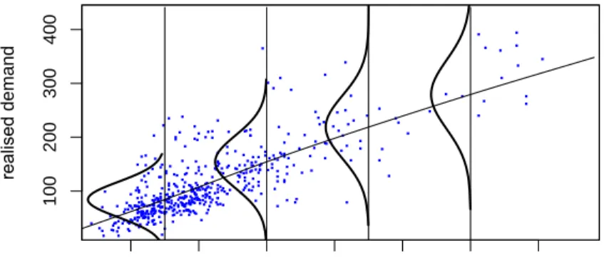
To fix these ideas, in Figure 5 we display a very simple GAMLSS, with normally distributed response, fitted to the demand data collected on the SKU grapes from September 2015 to August 2017, as shown already in Figure 4. More specifically, the model that was fitted is specified as follows:

yi∼N(µi,σi2)

µi=h1(xi)

log(σi) =h2(xi),

where yi is the i–th realised demand and xi is the median demand of the same

weekday in the previous month. The functionsh₁andh₂were estimated nonpara-metrically using P-splines. For notational simplicity, some indices were dropped here compared to the general model formulation in Equation (3).

The model displayed in Figure 5, while simplistic, adequately addresses the heteroscedasticity shown in Figure 4 by estimating the varianceσi2to increase for

increased values of the covariate. As a consequence, under such a model formulation, the cost-optimal inventory level at high covariate values would be farther away from the regression line than for small covariate values, thereby accounting for the increased uncertainty regarding customer demand. This pattern in the choice of the inventory level is in line with the theoretical results by Song (1994), who by means of stochastic comparison methods showed the impact of growing demand variability on optimal inventory levels and the corresponding economic costs.

50 100 300 350 100 200 300 400 150 200 250 realised demand

median demand same weekday previous month

Figure 5: Realised demand as a function of median demand of the same weekday of the previous month, together with the fitted GAMLSS, including the distribution implied for the residuals at selected values of the covariate.

3.2 Feature engineering

For all models, the demand distributionFt is estimated using features (explanatory

variables). Feature engineering describes the process of generating suitable features from data. Both the general pattern of the demand distribution as well as any time series effects are taken into account by considering historic demand quantiles (5%, 50% and 95%), then building corresponding features using data from a) the previous quarter, b) the previous month, and c) the previous two weeks (Lu, 2014 and Kawamura et al., 2015). After feature engineering and feature selection the data set contains the following 12 features, including also price (Andreyeva et al., 2010) and known demand as extracted directly from the raw data.

1. Demand of the same weekday previous week in units 2. Demand of the same weekday second previous week in units 3. Median demand of the same weekday previous month in units 4. Median demand of the same weekday previous quarter in units 5. Median demand previous month in units

6. Median demand previous quarter in units 7. 95%-demand-quantile previous month in units 8. 95%-demand-quantile previous quarter in units 9. 5%-demand-quantile previous month in units 10. 5%-demand-quantile previous quarter in units 11. Price

12. Known customer demand in units

These features were selected based on previous analyses in the literature as well as business experience made within the retailer considered in our case study, and aim at capturing,inter alia, time series effects and overall variation in demand. The choices made are thus somewhat arbitrary, which however seems necessary given the lack of clear guidelines on feature engineering in the context of e-grocery demand forecasting. In any case, for our real-data analysis — the purpose of which is to compare methods for demand forecasting — the selection of features is not of primary importance. Feature selection using component-wise gradient boosting, as described in Hofner et al. (2016), did not improve the out-of-sample forecast accuracy in our case study, so that we eventually trained all models using the complete feature set.

3.3 Benchmark models

Based on our literature review in Section 2.2, we consider linear regression (LM), quantile regression (QR), random forests (RF), and quantile regression forests (QRF) as performance benchmarks for the GAMLSS approach proposed here.

Linear regression models estimate the model parameters by minimising the sum of squared residuals. Based on a fitted linear regression model, we predict theconditional meanof the response distribution and, assuming normality of the residuals, derive the target quantile based on the estimated constant error vari-ance. Quantile regression methods directly predict anyconditional quantileof the response distribution (Koenker & Hallock, 2001). Random forests represent an ensemble learning technique that combines predictions from a specified number of tree predictors. Each tree is constructed independently by using a sub-sample of all observations available (Breiman, 2001). The output is again a prediction of the

conditional meanof the response variable. As a point forecast only, i.e. without accompanying distributional assumption for the residuals (such as the normal in case of basic linear regression), this prediction does not readily allow us to arrive at say the 0.97 quantile. In order to be able to compare the random forest-based prediction to the approaches that do provide us with quantiles, we thus complement the point prediction with an additional distributional assumption for the residuals, where for two-parameter distributions we simply use a constant standard deviation as estimated from one year of training data. For the random forest-based predictions we consider the same distributions as for GAMLSS (i.e. normal, gamma, Poisson, and negative binomial). Before applying the gamma distribution, we transformed the estimated mean and standard deviation to derive the required scale and shape pa-rameter. Finally, quantile regression forests constitute a nonparametric alternative to random forests that allows the estimation of anyconditional quantile(Meinshausen, 2006). The R packages we use arerq (Koenker, 2012) for quantile regression,

quantregForest(Meinshausen, 2006) for the quantile regression forest,caret(Kuhn, 2008) for random forests andgamlss(Rigby & Stasinopoulos, 2008) for GAMLSS. Thus, we apply the following benchmark models: Linear regression (LM); random forests with normal (RF NO); gamma (RF GA); Poisson (RF PO) and negative binomial distribution (RF NB); quantile regression (QR) and quantile regression forests (QRF).

4

Model training, demand forecasting and performance

evaluation

4.1 Training data

Our data set covers demand periods from September 2015 to August 2017 and six different e-grocery FC. We consider daily data, i.e. each demand periodtrefers to one day of delivery. For demand forecasting and hence validation of the different approaches considered, we use all demand observations from September 2016 to August 2017. We test five different SKUs within the SKU-category fruits, vegetables and meat, namely tomatoes, carrots, grapes, mushrooms and minced meat. All of these SKUs were listed for the entire period, exhibiting price changes throughout.

We train each model based on twelve months of data to subsequently forecast each demand in the following month. For example, we train each model based on data from September 2015 to August 2016 to forecast demand in September 2016. With a corresponding sliding-window approach, we always train on the most recent twelve months of data. In particular, the length of twelve months of the training data set allows the incorporation of seasonal effects. For each demand periodtand each of the parametric models considered, we obtain an estimate ˆFt for the demand

distributionFt, which we apply to deriveqt according to the newsvendor problem,

for any given demand quantile. For the nonparametric models that we consider — quantile regression and quantile regression forests — we deriveqt for selected

demand quantiles directly from the data, i.e. without previously having to build an estimate ˆFt. Thus, for each SKU we derive demand distributions for about 300

demand periods within the validation period, which results in>300K predictions ofqt when considering 11 models and 99 possible service levels.

4.2 Out-of-sample prediction of demand

Figure 6 illustrates the prediction step for the SKU grapes, showing the optimalqt

given a target service level of 97%, as obtained under each model, and additionally the realised demand, for the 23 demand periods in April 2017. We visualise the different model classes by different symbols and the different distributional assumptions by different colours. Since we derived the optimal inventory level

qt at the 97% service level target, qt should equal or exceed realised demand in

97% of all observations. But for our small subset of example prediction data generated by a single FC, four models, namely GAMLSS PO, RF GA, RF NO and RF PO, yield an inventory levelqt that is below realised demand for at least

two demand periods. Two demand periods with inventory levels below realised demand result in a service level of 91% (for this month). All other models yield inventory levels that in April 2017 never fall short of realised demand. Among these, considering overage costs for each excess unit of overage, we prefer inventory levels that are equal to or only slightly above realised demand. The inventory levelsqt

obtained from GAMLSS GA, GAMLSS NBI, QR and RF NB show high positive deviations from realised demand. Thus, in this small subset of predictions, the

models GAMLSS NBII, GAMLSS NO, LM and QRF appear to be most promising with respect to minimising total costs for the SKU grapes.

● ● ● ● ● ● ● ● ● ● ● ● ● ● ● ● ● ● ● ● ● ● ● ● ● ● ● ● ● ● ● ● ● ● ● ● ● ● ● ● ● ● ● ● ● ● ● ● ● ● ● ● ● ● ● ● ● ● ● ● ● ● ● ● ● ● ● ● ● ● ● ● ● ● ● ● ● ● ● ● ● ● ● ● ● ● ● ● ● ● ● ● ● ● ● ● ● ● ● ● ● ● ● ● ● ● ● ● ● ● ● ● ● ● ● ● ● ● ● ● ● ● ● ● ● ● ● ● ● ● ● ● ● ● ● ● ● ● 200 400 600

Monday Monday Monday Monday

realised demand for SKU grapes in the month April 2017

realised and estimated demand

● ● ● ● ● GAMLSS_GA GAMLSS_NBI GAMLSS_NBII GAMLSS_NO GAMLSS_PO LM QR QRF RF_GA RF_NB RF_NO RF_PO realised demand

Figure 6: Predicted 0.97 demand quantiles as obtained with the different approaches and realised demand for the SKU grapes in April 2017.

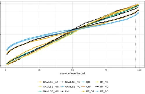
To obtain a more comprehensive picture, Figure 7 illustrates the overall deviation between the service level target and the realised service level for each model and each service level target between 1% and 99%. If a model would meet each service level target exactly, then the corresponding line would follow the 45◦ line. The figure demonstrates that the models GAMLSS PO, RF GA, RF NO and RF PO lead to substantial deviations for any service level target distinct from 50%, i.e. whenever costs are asymmetric. More specifically, below the 50% service level target, the inventory levels as obtained by these models are too high, whereas they are too low for all service level targets above 50%.

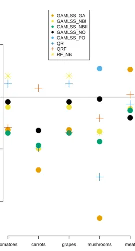
In practice, only the service level target of the e-grocery retailer is pertinent for model evaluation. Figure 8 shows the percentage deviation between the realised service level and the 97% service level target. For this particular service level, we observe that only the the model QRF obtains a service level target above 97%. Overall, we identify that the nonparametric models, QR and QRF, are closer to the service level targets than the parametric models, which would seem to corroborate the results of Sachs & Minner (2014). The models GAMLSS PO, RF GA, RF NO

●● ●● ●● ●● ●●● ●● ●● ● ●● ● ● ● ●● ● ● ●● ● ●● ● ●●● ● ●●● ●● ● ●● ●●● ●●● ● ●● ● ●● ●●● ●●● ● ●● ● ●● ●● ● ●●● ●● ●● ● ●●● ●● ● ●● ● ●● ● ●● ●● ● ●● ●● ●● ●● ●●● ● ● ●● ● ●● ● ● ●● ●●● ● ●● ● ●● ●●●● ●●● ● ●● ●●●● ●●● ●● ●●● ●●●● ●● ● ● ●● ●●●●● ●● ● ●● ●● ●●● ● ●● ●● ● ●● ●● ● ●● ●● ● ●● ●● ● ●● ●● ●● ●● ●● ● ●● ●●●●● ●● ●● ● ●●●● ●●●●●●● ●● ●● ● ● ●● ● ●●● ●● ●● ●●● ●● ●● ● ●● ● ● ●● ● ●● ● ● ●● ● ● ● ● ●● ● ● ●● ●●● ●● ● ● ●● ● ●●● ●● ● ● ●● ●● ● ●● ●● ●● ●● ● ●● ● ● ●● ●●●● ●●● ●●●● ●● ●●● ● ●● ● ●● ●● ●● ● ●●● ●●● ●● ●● ●● ● ●● ●● ● ●● ●●● ● ●● ● ●● ● ● ●● ●● ● ● ●● ● ● ●● ● ●● ● ●● ● ●● ●●● ●● 0 25 50 75 100 0 25 50 75 100

service level target

ser vice le v el realised ● ● ● ● GAMLSS_GA GAMLSS_NBI GAMLSS_NBII GAMLSS_NO GAMLSS_PO LM QR QRF RF_GA RF_NB RF_NO RF_PO

Figure 7: Service level target vs. realised service level for the SKU grapes in the validation period August 2016 to July 2017.

and RF PO show deviations of up to 17%. All other models show promising results in achieving the service level target with deviations below 6%, and hence are candidates for cost minimisation after considering asymmetric underage and overage costs.

4.3 Performance evaluation

Typical point forecast measures as applied in the existing literature, such as the mean average error (MAE) and the mean average percentage error (MAPE), assume a symmetric evaluation of the forecasting error (see, e.g., Makridakis & Winkler, 1983, Carbonneau et al., 2008). They are therefore inadequate to evaluate the

model performance for very high target service levels and hence asymmetric costs. Moreover, the MAPE is undefined for demand realisations of zero, which may occur for SKUs with intermittent demand in grocery retailing; see Kolassa (2016).

Since underage and overage costs are asymmetric in our business problem — and we thus have to evaluate the two directions of error asymmetrically — we aim

−15 −10 −5 0

GAMLSS_GA GAMLSS_NBI GAMLSS_NBII GAMLSS_NO GAMLSS_PO

LM QR

QRF

RF_GA RF_NB RF_NO RF_PO models

de

viation from 97% ser

vice le

v

el target

Figure 8: Model deviation from 97% service level target for the SKU grapes in the months August 2016 to July 2017.

to compare the out-of-sample forecasting error at the empirical service level target elicited from the retailer in our application. While specifying the numerical value of the overage cost parameterhis relatively straightforward given corresponding information from the retailer’s accounting department, this is not the case for the underage cost parameterb. Especially for relatively novel business models such as the one under consideration (e-grocery), the cost parameterbmust reflect the strategic objectives of the retailer and the financial consequences of medium and long term reactions of customers to stock-outs. The precise value of the parameterb

hence cannot be stated. Instead, we apply an indirect specification of the underage cost parameter bvia the relation α =b/(b+h) from the newsvendor problem, whereα is the service level. Given the empirical value of the service level and

an estimation of the overage cost parameterhbased on the retailer’s margin and operational costs, we derivebas

b= hα

1−α.

Given the resulting cost values forbandh, we then calculate the total costs that occur under theqt obtained from ˆFt for each demand periodtin the validation

period September 2016 to August 2017:

Ct(qt) =h(qt−dt)++b(dt−qt)+.

For each model, we sum up the costs for all demand periodst.

The asymmetric cost values ofbandhhave a strong impact on the evaluation of the relative model performance. Assuming, as an example, overage costs of 1 EURO and a service level target of 97%, we obtain underage costs of 32,30 EUR for each unit of underage. Thus, a method that overestimates demand by 32 units generates (slightly) lower costs than an alternative method that underestimates demand by one unit.

5

Results

Figure 9 shows the percentage difference in total costs, according to (1), as obtained under the different approaches, in each case compared to the benchmark linear regression:

perc. diff. in total costs=100

Ct(q∗t) Ct(qLMt ) −1 ,

whereq_tLMandq∗_t are the optimal inventory levels according to linear regression modelling and the alternative method under consideration, respectively.

For all SKUs considered, we find that models from the GAMLSS class outper-form the benchmark models, with different distributions across the different SKUs yielding the lowest out-of-sample costs. Compared to linear regression, we find potential cost reductions of up to 25%. The results indicate that at least one of the assumptions made within basic linear regression, such as homoscedasticity or normality, will typically be violated in this kind of data. GAMLSS allows us to tailor the regression model to whatever pattern we find for a given SKU, such that, as expected, in most cases it leads to improved demand forecasts. An exception is the model GAMLSS PO, which in terms of its single-parameter response distribution is actually less flexible than a basic, possibly non-linear regression model — the im-plied mean-variance relation of the Poisson here drastically limits the model’s ability to capture the empirical patterns. Overall, the results demonstrate the strengths of

−20 −10 0 10 SKU percentage diff

erence in percentage costs compared to LM

tomatoes carrots grapes mushrooms meat ● ● ● ● ● ● ● ● ● ● ● ● ● ● ● ● ● ● ● ● ● ● ● ● ● ● GAMLSS_GA GAMLSS_NBI GAMLSS_NBII GAMLSS_NO GAMLSS_PO QR QRF RF_NB

Figure 9: Relative total costs as obtained under the different approaches, compared to the benchmark linear regression, for five different SKUs.

GAMLSS by allowing a flexible selection of distributions for the demand, and also a flexible modelling of covariate effects on any of the distributional parameters. However, it is worth noting that there is no distributional assumption within the class of GAMLSS that performs best across all SKUs in our case study. This is perhaps not surprising given the wide range of demand patterns of SKUs on offer (e.g. fast-moving or slow-moving SKUs with regular or irregular demand).

of distributions. However, with our somewhat ad hoc approach to complement the point forecast by a distributional assumption for the residuals, the estimated standard deviation from historic data is constant over time. As a consequence, this type of approach cannot accommodate heteroscedasticity, which however is crucially important when trying to capture the extreme (right) tail of the demand distribution. Random forests do indeed yield much higher costs across all distributions considered. In contrast to random forests, the quantile regression-based approaches performed very well in our case study. However, due to their sensitivity especially for extreme quantiles (e.g. 0.99), they still do bear the risk of occasionally producing demand forecasts that are way off. In addition, it can be disadvantageous that these models need to be fitted separately for any target quantile considered. In other words, as distribution-free methods, they do not allow practitioners to select the inventory level based on eyeballing a demand forecast distribution.

In our view, interpretability in retailing practice is in fact an important benefit of the GAMLSS class. In retail practice, the interpretation of demand forecasts, and how they were obtained, is a relevant requirement of the operational management since it allows the inclusion of expert knowledge for forecast adjustments in the case of exceptional circumstances (cf. Fildes et al., 2009, Davydenko & Fildes, 2013). In particular, machine learning techniques are often restricted in their possibilities of interpretation. In contrast, practitioners familiar with basic regression can be expected to relatively easily grasp the concepts of distributional regression — after all, in most of the corresponding models the main difference to linear regression is simply that we model not only the mean but also the variance. In any case, the resulting cost-optimalqt can directly be “read” from the forecast distribution

as implied by the fitted GAMLSS. To illustrate this point, Figure 10 presents the GAMLSS with normally distributed response fitted to the data collected on the SKU grapes, here showing the associated forecast distributions for each weekday in the demand period 24-07-2017 to 29-07-2017. The model captures the fact that demand peaks at the beginning of a week, but also accounts for the associated increased variance in demand. The latter information would not readily be available when using quantile regression methods, as these target only at specific points of the forecast distribution, namely the quantiles of interest. Thus, the GAMLSS approach provides a more comprehensive picture of the demand to be expected.

0 100 200 300 400 500

demand forecast distribution under GAMLSS_NO

monda y ● 0 100 200 300 400 500 tuesda y ● 0 100 200 300 400 500 w ednesda y ● 0 100 200 300 400 500 thursda y ● 0 100 200 300 400 500 fr ida y ● 0 100 200 300 400 500 saturda y ●

Figure 10: Demand forecast distribution for the SKU grapes under the model GAMLSS NO in the week 24-07-2017 to 29-07-2017; the 97% quantiles under each daily forecast distribution are highlighted in blue.

6

Conclusion and future research

In this paper, we present a case study for distributional demand forecasting in e-grocery. For highly perishable SKU with complex demand patterns, we find that models from the GAMLSS class tend to outperform the benchmark models, which is due to their increased flexibility in accommdating complex demand patterns. While our work was motivated by the new types of data found in e-grocery retailing, in particular uncensored demand and known demand at replenishment order time, all methods considered are, in principle, also applicable to traditional retail practice. While the performance of the GAMLSS class in our case study is promising, we