LUMA-GIS Thesis nr 11
Advanced Decision Support Methods for
Solving Diffuse Water Pollution Problems
Svajunas Plunge
2011
Department of Earth and Ecosystem Sciences
Division of Physical Geography and Ecosystem Analysis Centre for Geographical Information Systems
Lund University Sölvegatan 12 S-223 62 Lund Sweden
Advanced Decision Support Methods for Solving
Diffuse Water Pollution Problems
Svajunas Plunge
Department of Physical Geography and Ecosystem Analysis Lund University, Sweden
Master thesis 30 credits, in partial fulfillment of the requirements For the degree of
Master in Geographical Information Science Supervisor: Andreas Persson
Abstract
Dealing with water diffuse pollution is a major problem for watershed managers. This problem raises many complicated questions, which are important to answer in order to reach water environment protection goals. This study suggested some possible answers for the country of Lithuania. Among them were the identification of critical source areas, the identification of sensitive areas and the application of multi-objective spatial optimization. Those decision support methods were not only suggested, but also examined through literature review and their application was demonstrated practically on the Graisupis river catchment, which is located in the middle of Lithuania. For this purpose, the SWAT (Soil and Water Assessment Tool) model was prepared and successfully calibrated and validated for water flows and nitrate load simulations. The model was calibrated for 7 years (2000-2006) and validated for 3 years period (2007-2009). The model was run for 10 years period (2000-2009) in order to obtain results for decision support methods. Critical source areas were defined as those areas, which have nitrate loads to surface water bodies higher by two standard deviations from average in the catchment. Sensitivity (nutrient leaching potential) of areas was assigned based on the response of modeled physical nature to the addition of nitrogen fertilizers. The SWAT model was also used for the simulation of effects of best environment practices. The results were imported into the genetic algorithm, which was used for the purposes of multi-objective spatial optimization. Model results indicated average nitrate loading of 15.9 kg nitrate nitrogen per hectare in the catchment. The identification of critical source areas located 12.4% of the Graisupis river catchment as risk areas. The sensitive areas identification assigned medium or low sensitivity to 99.5% of the catchment. Only 0.4% of the catchment territory was identified as high or very high sensitivity. Multi-objective spatial optimization increased the cost-effectiveness of diffuse pollution abatement 24 times (up to 50 times with lesser implementation scale), if compared to the random selection of best environmental practices. Optimization with equal weights for environmental and economic objectives resulted in 16.9 LTL for reduction of 1 kg nitrate nitrogen to surface water bodies, while providing 62% reduction of total loads to surface water bodies. This scenario required 24% of additional catchment territory to be converted to grasslands and consideration of filter strips for 34% of the catchment territory. Optimization for obtaining Pareto optimum between environmental and economic objectives provided the most cost effective solution of 9.7 LTL for reduction of 1 kg nitrate nitrogen, while providing 25% reduction of total loads to surface water bodies. This scenario required the application of cover crops on 2.6%, new grasslands on 1.6% and consideration of filter strips on 11% of the Graisupis river catchment area. Optimization for obtaining Pareto optimum between environmental and economic objectives also provided quantifiable relationship between economic and environmental objectives in the form of regression equation.
Key words: diffuse pollution, non-point pollution, critical source areas, sensitive areas, multi-objective spatial optimization, best environmental practices, best management practices, SWAT model, Lithuania.
Acknowledgements
I would like to thank Dr. Ausra Smitiene for providing valuable comments and important data for the model preparation.
I would also like to thank the administration of the Lithuanian Environmental Protection Agency for allowing me to complete the model preparation part during working hours.
List of Abbreviations
BEP1 – Best Environmental Practice BMP2 – Best Management Practice CSA – Critical Source Area
DEM – Digital Elevation Data
FAO – Food and Agriculture Organization GA – Genetic Algorithms
GIS – Geographical Information Systems HRU – Hydrological Response Unit
HWSD – Harmonized World Soil Database
LEPA – Lithuanian Environmental Protection Agency LHMS – Lithuanian Hydrometeorological Service MOSO – Multi-Objective Spatial Optimization PEM – Point Elevation Data
PI – Phosphorus Index
SWAT – Soil and Water Assessment Tool USLE – Universal Soil Loss Equition WMI – Water Management Institute
1 BEP used in the European context.
Table of Contents
Abstract...iii Acknowledgements...iv List of Abbreviations...v Preface...1 1 Introduction...12 Goal, Objectives, Scope and Delimitations...2
2.1 Goal...2
2.2 Objectives...2
2.3 Scope/Delimitations...2
3 Work Flow...3
4 Literature Review...5
4.1 Identification of Critical Source Areas...5
4.1.1 CSAs Definition...5
4.1.2 Importance of CSAs...6
4.1.3 Simple Methods for CSAs Identification...6
4.1.4 Advanced Methods for CSAs Identification...7
4.1.5 General Problems Connected to the Use of CSAs...8
4.2 Multi-objective Spatial Optimization...8
4.2.1 Genetic Algorithms...9
4.2.2 Other Factors to Consider in an Optimization ...11
4.2.3 Relation to CSA...11
4.2.4 Environmental versus Economic Objectives...12
4.3 Summary of Literature Part ...13
5 Method Application...14
5.1 Model Selection...14
5.2 Area Discription...14
5.3 Data and Parameters...15
5.3.1 Data Inputs...15
5.3.2 Estimation of Soil Parameters...19
5.3.3 Data Adjustments...20
5.4 Model Preparation...21
5.4.1 Dividing the Catchment...21
5.4.2 Calibration of Flow...22
5.4.3 Validation of Flow...26
5.4.4 Calibration of Nitrates...26
5.4.5 Validation of Nitrates...29
5.5 CSAs and Sensitive Areas Identification...31
5.6 GA Preparation and Spatial Optimization...32
6 Results...35
6.1 CSAs and Sensitive Areas...35
6.2 Multi-objective Spatial Optimization...38
7 Discussion...43
8 Conclusions...45
Reference list...46
Appendix A...51
Preface
Ideas for this work came from the problems I encountered when working in the Lithuanian Environmental Protection Agency (LEPA). This work has been intended as a demonstration how some of those problems could be solved. Although to apply the suggested solutions on the country basis would require much more work to be done and more specialists to be involved, decision making for watershed management would reach the new level in Lithuania if these solutions were applied. This level is of sound science and methods application in decision support. Hopefully, this work will be a stepping stone to this direction.
1 Introduction
Diffuse water pollution is the biggest challenge for watershed managers if the deterioration of water ecosystems is going to be stopped and reversed. Current legislation such as Water Framework Directive (European Union) and Clean Water Act (USA), require substantial improvement of water quality. This is not possible without solving diffuse pollution problem. Compared to point source pollution (solved by the installation of waste water treatment plants, as well as change in chemical use and technologies), a successful solution for diffuse pollution requires much more complicated approaches. It requires the application of Best Management Practices (US terminology) or Best Environmental Practices (EU terminology) in the right complexes and in the right places. Even though a more intensive application of abatement measures would increase the possibility to reach the desired result, due to financial constraints, lesser scale of abatement is desired. In order to combine both environmental and economical goals in one assessment some kind of multi-objective functions are needed. They should also be integrated with spatial optimization techniques. This kind of approach is vitally needed, especially in Lithuania (my country of origin). The implementation of River Basin Management Plans for the Water Framework Directive should start at the latest in 2012. Yet, until this day (the final stage of the preparation of River Basin Management Plans) there is no clue how the placements and types of different diffuse pollution abatement measures will be selected on a field level. There is only a vague understanding how much tons of nitrogen or phosphorus should be reduced per watershed. If no guidance is available, diffuse pollution abatement will result in random application of abatement measures, thus causing ineffective use of funds designated for the protection of water ecosystems. This work is designated for addressing this problem.
2 Goal, Objectives, Scope and Delimitations
2.1 Goal
The main goal of this study is twofold. The first is to develop and apply a decision support method for the identification of critical source areas (CSA) for non-point sources and sensitive areas for pollutants in a selected watershed of the Lithuanian river. The second is to develop and apply a multi-objective spatial optimization (MOSO) technique for the selection and placements of best environmental practices (BEPs).
2.2 Objectives
Three broad objectives have been raised in order to reach the goal of this study. First, to make an analysis of literature related to the identification of CSAs and the application of MOSO techniques for diffuse water pollution problem solution. Second, to prepare a selected physically-based, distributed or semi-distributed watershed model on the selected watershed in Lithuania. Third, to develop and apply methods for CSA, sensitivity identification and MOSO.
2.3 Scope/Delimitations
This work is mainly intended to serve as a demonstration to watershed managers how analyzed problems could be solved. Model preparation and analysis parts were made according to literature and known practices. However, if the results should be applied for management purposes, more detailed local data are needed in regard to soil parameters, fertilization, tillage, economic values and wider range of BEPs should be considered as well. It is also important to mention that literature analysis on sensitivity identification techniques was skipped, because it was only a minor objective and ideas for it were quite clear from the beginning. Model selection and preparation have been build on the knowledge and skills gained from the previous work of Plunge (2009).
3 Work Flow
The sequence of activities done are presented in Picture 1. They are reflecting 3 main objectives raised for the study. Literature review and model preparation were done simultaneously. As model and area selection has been based on the previous work of Plunge (2009), it was possible to do the model preparation together with literature review. A literature analysis for CSA and MOSO themes (attached to diffuse surface water pollution problems) was made. The model preparation stage was the most time consuming. It was performed in steps. Firstly, the required datasets and parameters were gathered from various institutions, LEPA being the main source. Then, data were converted to the right formats, and missing parameters were estimated. This was needed for the model setup stage and running the model. Probably the most time consuming stage was model calibration. Although initial SWAT runs were showing satisfactory results and SWAT-CUP program helped a lot in calibration, many things had to be corrected before good results could be produced. The model was calibrated for water flows and nitrate loads. Model validation was done after calibration.
Literature review provided necessary knowledge and ideas for the application of methods stage. Specifically, literature review gave input to the identification of CSAs and the application of MOSO. The application of methods began with the selection of BEPs and the simulation of selected scenarios. Selection of BEPs was based on three criteria: suitability for simulation with the prepared model, possibility for installation on the selected watershed and availability of economic values. During simulation of scenarios, the selected BEPs as well as baseline and land response to nitrogen fertilization were evaluated . The results from simulation of scenarios provided input to the identification of CSAs, identification of sensitive areas and preparation of BEPs database. BEPs database consisted of loadings for each HRU under each scenario, which came from the simulation of scenarios with the prepared model. BEPs database also consisted of cost values for each HRU under each scenario. The application of MOSO technique was the last step in the application of methods stage. During this step a genetic algorithm was developed and used in the optimization of BEPs placement. The final results are shown in maps and the Pareto optimum graph. The analysis of results stage was used for the discussion of findings.
Picture 1: Work flow of the study. A p p lic at io n o f m et h od s M od el p re p ar at io n Literature review
CSA MOSO Data and parameters gathering
Model setup Calibration and validation Identification of CSAs Preparation of BEPs database Selection of BEPs Application of MOSO technique Identification of sensitive areas Analysis of results Simulation of selected scenarios
4 Literature Review
Literature review was narrowed to the topics relevant to the study. Two questions were examined. One is the identification of CSAs for the purposes of diffuse water pollution management. Second is the application of MOSO for solving questions of BEPs selection and distribution questions.
4.1 Identification of Critical Source Areas
Understanding of the inland surface water diffuse pollution phenomenon requires to have good knowledge about processes occurring in a watershed. Spatial dimension is essential for this understanding. In order to effectively tackle diffuse pollution it is necessary to locate the most important source areas of pollutants effecting water bodies. They are often called critical source areas (CSAs).
4.1.1 CSAs Definition
In general CSAs are defined as areas, which “contribute most pollutant load of the entire watershed and have a decisive impact on the receiving water quality” (Ou & Wang, 2008). However to define CSAs in practice is not as straightforward. There are many possible ways, which were found in literature.
The first problem is how to define “a decisive impact” on the water quality in a watershed. In other words, how to transform qualitative terms into to quantitative terms. Scientific literature provides a number of examples for solving this problem. For instance, White et al. (2009) define CSAs for sediment and phosphorus yield by ranking discrete units comprising the watershed according to their predicted contribution to the total load of sediment and phosphorus yield. 2.5% and 5% of total loads were chosen as benchmarks for CSA identification. Tripathi et al. (2003) defined CSAs for soil loss as sub-watersheds where predicted soil loss exceeded the “tolerable” level of 11.2 t/ha per year, which was based on previous studies in that area. CSAs identification for nutrients was based on threshold values for nitrate nitrogen and for dissolved phosphorus loading to water bodies, which were 10 mg/l and 0.5 mg/l. Those values were obtained from US EPA Quality Criteria for Water of 1976. Sivertun & Prange (2003) divide CSAs into risk and sub-risk areas. Risk areas are defined as areas, which obtain values of loadings higher than the mean value by two standard deviations and sub-risk areas as areas, which obtain values higher than the mean value by one standard deviation.
Another important aspect in the definition of CSAs is the spatial scale or spatial elements for which CSAs are defined. In general, the identification of CSAs is desirable on as detailed scale as possible. However, this might be very tricky. Therefore in some studies (Tripathi et al., 2003, Ouyang et al., 2008) critical sub-watersheds instead of critical areas in the watershed are identified. In other studies (White et al., 2009, Srinivasan et al., 2005) hydrological response units3 (HRUs) are the basis for CSAs identification. In GIS based methods a raster cell is often used as the unit on which calculations and CSAs identification is obtained. Examples of this can be found in the articles of Sivertun & Prange (2003) and Ou & Wang (2008).
It is also necessary to consider the perspective when defining CSAs. According to Mass et al. (1985), CSAs can be defined from the land resource perspective and from the water quality perspective. Land resource perspective emphasizes the importance of those areas where soil erosion 3 Hydrological response units represent areas within sub-basin with unique combination of soil, land use and slope
is higher than could be tolerated. Water quality perspective points to the areas where the best management practices (BMPs) could achieve the greatest improvement with the lowest cost.
Lastly, it is important to mention that ideal criteria for CSAs definition should encompass hydraulic transport of pollutants to a watercourse, magnitude of pollutant source, type of water resource and type of pollutant (Watershedss, 2010). In some cases, the identification of CSAs for certain pollutants is based on CSAs on other pollutants (as carrying vectors) or on CSAs defined for generating surface runoff. For instance, areas with increased soil loss would definitely have increased loadings of sediments and nutrients on the surrounding water bodies (Sivertun & Prange, 2003). According to Srinivasan et al. (2005) areas with increased surface runoff could be used to identify CSAs for phosphorus. Some authors (Qiu, 2009, Rao et al., 2009) suggested that CSAs for phosphorus and related pollutants could be approximated by variable sources areas (areas that actively generate runoff).
4.1.2 Importance of CSAs
The importance of CSAs for diffuse pollution abatement is well stressed by many authors (Qiu, 2009, Trevisan et al., 2010, Strauss et al., 2007, Diebel, et al., 2008, Ouyang et al., 2008, Tripathi et al., 2003, White et al., 2009, Noll & Magee, 2009). The contribution of pollutant loads is not uniformly dispersed in watersheds. Some areas have much greater influence on water bodies than others. For example, in the study made by White et al. (2009) 5% of that land area was responsible for 50% of sediment loads and 34% of phosphorus loads. Another example is the study made by Diebel et al. (2008) on Hefty Creek watershed in Wisconsin (USA), which concluded that 26% of phosphorus loss reduction could be achieved by targeting conservation measures to only 10% of fields. White et al. (2009) concluded that loads from CSAs were 3 to 10 times higher compared to average loads from agricultural fields. Therefore, it is quite obvious that in order to increase effectiveness of BEPs, abatement measures should be targeted on CSAs.
The significance of CSAs has been recognized by governmental institutions as well. For instance identification of CSAs is required for the projects of the US Rural Clean Water Program (Watershedss, 2010). The requirement for CSAs identification is primarily related to the requirement for cost-effectiveness of the selected abatement measures. According to Gitau et al. (2004) effectiveness of BMPs is significantly related to their placement in a watershed. Thus, it is possible to conclude that CSAs identification is one of the most important steps in inland surface water diffuse pollution abatement.
4.1.3 Simple Methods for CSAs Identification
Methods for CSAs identification can be divided into two broad categories, i.e. simplified and advanced methods. Simplified methods or models usually just show possible risk areas, whereas expert models or on-site exploration provide a more detailed analysis as well as quantities of pollutants coming from CSAs (Sivertun & Prange, 2003). Simple methods are fast, relatively cheap, requires little data and can be easily applied on large areas. They are often used in a screening stage. An example of the simplest method for CSAs identification is the designation of all croplands within a quarter mile of water bodies to CSAs (Watershedss, 2010). Also CSAs can be identified on a sub-watershed level based on how much of the watershed is covered by agricultural lands (Minister of Environment of the Republic of Lithuania, 2005). Two most widely known (and used in practice) simple CSAs identification methods are phosphorus index (PI) and universal soil loss equation (USLE) model. PI was developed by US researchers. This method uses fertilization rate by phosphorus, phosphorus in soil, size of livestock, population density, transport factor, soil erosion,
distance to stream, surface runoff and other factors (depending on version of PI) to come up with the index number, which would allow the indication of increased phosphorus load areas (Ou & Wang, 2008). By overlaying different factors in GIS analysis it is possible to identify risk areas or CSAs for phosphorus. The final PI value has no physical meaning, however, it allows comparison between the areas. USLE allows to estimate annual average soil loss (in tonnes per acre or hectare) that occurs due to sheet or rill erosion (OMAFRA, 2000). Calculation of soil loss is done by multiplication of rainfall/runoff, soils erodibility, slope length-gradient, crop/vegetation and management, and support practice factors. There are different adaptations of the USLE model. Sivertun & Prange (2003) developed the GIS USLE model, which is used for the identification of risk areas in much the same way as PI. Huang & Hong (2010) combined soil conservation service curve number (SCS-CN), USLE and nutrient losses equations into GIS based empirical model and applied it to identification of nitrogen and phosphorus CSAs.
Other examples of simple methods are erosion index and sediment yield index (Tripathi et al., 2003). A fuzzy modeling technique or simple overlays in GIS can be used for the identification of CSAs. Professional judgment by conservation managers can also be applied for qualitative evaluation of CSAs (White et al., 2009). There are many other methods as well.
Despite many benefits of using simple methods for the identification of CSAs (such as simplicity of analysis, low cost and time saving), there are many drawbacks, which should be addressed. The majority of simple methods are not capable of providing physically meaningful quantitative results because they do not represent actual physical processes occurring in an environment (Srinivasan et al. 2005). Index values allow comparison between the analyzed areas, however the extent of problems is beyond grasp of these methods. Moreover, there are many other restrictions in the use of simple methods. For example, according to Sivertun & Prange (2003), limitations of the USLE model are the following: factors for this model are only valid for areas that are similar to the areas, which were used in the development of the USLE model; the model could only analyze erosive slope parts and not accumulative; the model is applicable only to straight slopes, concave and convex slopes should be sub-divided to be included into this model. These and other problems determined that the attention is being focused on advanced methods for CSAs identification.
4.1.4 Advanced Methods for CSAs Identification
Advanced methods are used after screening stage, ideally for areas, which was identified as the areas of concern. Main distinction from simple methods are complexity of them (more than a single equation). Those methods encompass on-site exploration4 and expert models. Expert models for CSAs identification are physically based models suitable for inland surface water diffuse pollution modeling. There are many examples of them, however to review all them is outside the scope of this study. Since this work was build on previous work of Plunge (2009), which selected SWAT model among other tools for diffuse pollution modeling, further discussion would focus on the SWAT model application for CSAs identification.
The SWAT model is one of the most widely used and robust physically based models for the assessment of diffuse pollution problems (Gassman et al., 2007, Srivinasan et al., 2005). Moreover, it has been integrated into GIS environment of ArcGIS (proprietary software) and Map Window (open source software). This is the key characteristic for the usefulness of such tool in CSAs identification. The successful application of SWAT for the purpose of CSAs identification has been demonstrated by many authors (Ghebremicheal et al., 2010, Srinivasan et al., 2005, White et al., 2009, Tripani et al., 2003, Ouyang et al., 2007). Most of them concluded that the SWAT model is a suitable tool for directing management efforts in abating diffuse pollution.
However, a few problems have been raised in the studies examining the application of the SWAT model for the CSAs identification. The most important one is that the SWAT model does not simulate overland routing of pollutants and runoff (Srinivasan et al., 2005). This is due to the model concept, which treats loads within the sub-basin identically, disregarding their position of origination (White et al., 2009). This simplification increased the model's speed greatly, however, it reduced its capability to represent an environment in more detail. The SWAT model is good for predictions on a watershed scale, however, it was not designed for pollutant routing predictions at the detailed level. Nevertheless, according to White et al. (2009) correction of this shortcoming is planned in future versions of the SWAT model. Meanwhile this problem can be reduced by reducing size of sub-basins during watershed configuration stage. Other problems are connected with spatial calibration and validation of the model, data needs, etc. However, despite of these problems the application of the SWAT model for CSAs needs is highly recommended by the scientific community (Srinivasan et al., 2005, White et al., 2009, Tripani et al., 2003, Ouyang et al., 2007).
4.1.5 General Problems Connected to the Use of CSAs
There are also some general problems connected with CSAs identification and the concept itself, which should be discussed. Firstly, it must be mentioned that although many studies have identified CSAs, it is very hard to find studies, which would validate their methods with field experiments or measurements. According to White et al. (2009), “there is no quantitative assessment of program effectiveness if CSAs are actively targeted”. Another problem is that very few simple methods provide physically meaningful quantitative results. Even if some methods can do this, uncertainty of the results obtained is very large. On the other hand, advanced methods usually have no official guidance how models should be used in the identification of CSAs. Since watershed modelers prepare models with different assumptions, different parameter sets, etc., there is no guarantee that the same (or at least similar) results will be obtained by different watershed modeling specialist even if they use the same model on the same areas and for the same time period. Thus comparison between studies is complicated. Also the importance of hydrological pathway is rarely well integrated into the methods used for CSAs identification (Watershedss, 2010). This is causing questions about the validity of results. There are other problems as well. Nevertheless, CSAs and their identification are the key component on any plan to abate inland surface water diffuse pollution.
4.2 Multi-objective Spatial Optimization
The effectiveness of BEPs for the control of diffuse pollution depends not only on the suitability of the site, but also on the right selection of BEPs. Those two factors affect the cost-effectiveness of diffuse pollution abatement programs the most. For finding an optimal distribution of BEPs as well as their optimal composition (in order to reduce abatement costs) multiple scenarios should be compared. However, this comparison is not possible with conventional methods. To find an optimal solution one should consider an exponential number of possible scenarios. According to Veith et al. (2003), for four nonmutually exclusive BEPs considered in 50 fields on some watershed, the number of possible scenarios would be (24)50. The on-site selection of BEPs is neither practical nor economically feasible with such a number of possible options. In addition to this, field studies could not aid much in solving this problem. Establishing BEP effectiveness for a particular scenario takes many years. Yet, results are site specific and dependent on temporal variability in climatic conditions in that specific area (Veith et al., 2004). Moreover, multiple and often conflicting objectives should be combined when planning diffuse pollution abatement. Environmental,
economical, sometimes institutional, esthetic and maybe even other types of objectives are equally important. Thus, finding solutions to such complicated problems seems to be an impossible task. No surprise that currently the placement of BEPs for abating agricultural diffuse pollution is done largely at random (Gitau et al., 2004, Maringanti et al. 2009). Yet, increasing numbers of studies have been done to solve this problem. They commonly apply techniques, which can be assigned to the group of multi-objective spatial optimization (MOSO) methods. Those methods integrate GIS, some kind of diffuse pollution modeling, an economical analysis and the most important, selected optimization methods.
Optimization problems are solved with many different methods: goal programing, linear programing, response surface methodology, shuffled complex evolution, simulation annealing, tabu search, genetic algorithms (GA) and others. These methods come from and are used in different disciplines: economics, engineering, informatics, mathematics, biology, evolution, etc. Despite this abundance of methods, most of the reviewed studies (Veith et al., 2003, Veith et al., 2004, Gitau et al., 2004, Maringanti et al., 2009, Arabi et al., 2006, Jha et al., 2009) used GA for the BEPs' optimization purposes in watersheds. For all of these studies GA usage was successful. The effectiveness and easiness of the MOSO problem formulation makes GA the most common choice. Therefore, only this method will be presented in more detail.
4.2.1 Genetic Algorithms
Genetic algorithms (GA) is the group of methods inspired by evolutionary biology. They are using the same principles of selection, inheritance, crossover and mutation, as life used for its evolution. Picture 2 presents the example of basic framework for GA, which can be also applied to watershed problems.
Each scenario for a watershed in GA is represented by a chromosome. A chromosome represents an individual in a population. A chromosome is composed from genes. Genes have information about the choice of management options for a certain field (it could also be a HRU or a
sub-Picture 2: General framework for GA (EDC, 2010). Create population of
chromosomes Determine the fitness of
each individual
Select next generation Perform reproduction using crossingover Perform mutation Display results next generation generation = 0 final generation
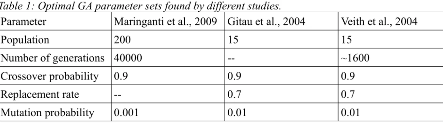
watershed). Each gene has possible allele sets. They are alternative management options for the same field. A selected number of initial individuals (represented by chromosomes) is randomly generated. During generations individuals with the highest fitness score are selected for breeding. During breeding the chromosomes of two individuals exchange parts through the process called crossover and two new chromosomes are formed. During each generation the lowest rated individuals (based on their fitness score) are removed from the population. In this way, the optimal solution is found after many iterations (generations in GA terminology). However, it is possible that this method would end up in local optima instead of global optima. Therefore, a mutation (random changes of genes) is introduced. Its probability should be low enough to keep the optimization results within the population, yet large enough to prevent convergence to local optima. The mutation rate for watershed studies of 0.01 has been proposed by Gitau et al. (2004) and Veith et al. (2004), whereas Maringanti et al. (2009) found the optimal gene mutation rate for its study to be at rate of 0.001. Other important parameters such as population and generations number greatly varies between mentioned studies, while optional parameters such crossover probability5 and replacement rate6 are based on the same values. All GA parameters of the mentioned studies are presented in Table 1. Even if GA parameters are specific for each study, this information could be helpful to get ideas about the choice of initial parameters when preparing GA.
Table 1: Optimal GA parameter sets found by different studies.
Parameter Maringanti et al., 2009 Gitau et al., 2004 Veith et al., 2004
Population 200 15 15
Number of generations 40000 -- ~1600
Crossover probability 0.9 0.9 0.9
Replacement rate -- 0.7 0.7
Mutation probability 0.001 0.01 0.01
Other important factors to consider when preparing GA are termination criteria, allele sets and the type of GA linking with other components of optimization. Termination criteria can be defined either by the maximum number of iterations or by minimal improvement in the maximum fitness score. Both criteria can be used at the same time. It may be also important to define possible allele sets (management options) for each land use type or HRU. This is essential, since each land use type has only a certain group of applicable BEPs, which could be implemented or might be considered for implementation on this land use type.
A GA linkage with other components may be static or dynamic. A static linkage uses results of other components not linking them directly during the GA optimization. Dynamic linkage usually integrates the pollution simulation model and GA in the same simulation. The benefit of dynamic linkage is that pollutants routing can be accounted in the optimization. However, the dynamic linkage makes the optimization so much slower, that it can be used just on very small watersheds. In the study of Maringanti et al. (2009), static linkage was used and routing was not considered in the optimization. Authors argued that the inclusion of in-stream processes was not significantly changing optimization results. Therefore, routing could be excluded from the optimization with the benefit of increasing optimization speed.
Lastly, it is necessary to mention that the term GA can refer to the optimization method and to the optimization program. Scientists often write the code for GA programs by themselves or use the 5 Crossover occurs with defined probability during breeding.
prepared one. For example, in the study of Perez-Pedini et al. (2005) the commercially distributed GA program Evolver© (http://www.palisade.com/evolver/) was used. Gitau et al. (2004) and Veith et al. (2003) used the freely available GALib package (http://lancet.mit.edu/ga/).
4.2.2 Other Factors to Consider in an Optimization
A few other factors, which have not been mentioned above, should be taken into account when preparing MOSO. Optimization is usually done by the integration of several tools. One of them is GA, another might be the watershed model and the third one might be the BMP tool7. In the studies of Maringanti et al. (2009) and Gitau et al. (2004), the BMP tool has been used as a component incorporated into optimization. According to Miringanti et al. (2009), “the BMP tool is a database that contains the quantitative information regarding the effectiveness of a BMP to reduce a particular pollutant from a given land use”. The BMP tool of Gitau et al. (2004) study contained 32 BEPs, which, according to the authors, could be divided into eight classes, such as animal waste systems, barnyard runoff management, conservation tillage, contour strip crop, crop rotation, vegetated filter strips, nutrient management plans, and riparian forest buffers. BMP tools are developed in two ways. Either the BMP tool is based on the results from BEPs monitoring studies as is in Gitau et al. (2004) or it is made by employing models as in the study of Miringanti et al. (2009). Miringanti et al. (2009) used the SWAT model for the simulation of the baseline (scenario without BEPs) and then simulated each BEPs separately on the selected group of HRUs. From this information authors calculated the effectiveness of each BEP on HRUs for which this BEP could be applied.
One more component necessary for MOSO is BEPs costs information. Some kind of database of annualized cost should be incorporated into optimization. The previous section (on environmental versus economical objectives) presented the discussion about what information should be included into this component.
Another important factor, which should be considered in MOSO, is how final results will be obtained. Is it by using a single objective function or Pareto optimum? The single objective function has an advantage of providing one answer that is straightforward to translate to spatial dimension. Whereas Pareto optimum provides multiple solutions, which are equally good. Thus, it is not as straight forward to provide one nice looking final map. However, according to Miringanti et al. (2009) these multiple near-optimum solutions are a great advantage over the single-objective function, since it allows decision makers to get insight into trade-offs between different solutions. The final result can be translated to map after decision makers decide, which solution is suitable for them.
Finally, it is important to mention the influence of uncertainties in MOSO. It is generally ignored by most of the studies. No surprise, since it would complicate the optimization process even further. However, according to Meyer et al. (2009), the influence of uncertainties is largely overlooked and the exclusion of them from the analysis could introduce far higher errors in the final results than one might expect. For more discussion on uncertainties and the use of uncertainty analysis in watershed studies please refer to Plunge (2009).
4.2.3 Relation to CSA
Before examining MOSO methods and their use, it is important to understand their relation with CSA, since it is another important part of this work. In the article of Veith et al. (2004), this link has 7 It should be called the BEP tool in the European context. However articles, which mention it, are only American.
been provided. Authors divide all methods for the selection of BEPs applications into plan-based and performance based methods. Plan-based methods are built on past field studies and scientific theory. This category includes targeting methods, which direct diffuse pollution abatement towards CSAs. On the other end there are performance based methods, which apply simulation models to assess the effectiveness of various scenarios of BEPs application. Optimization methods are assigned to the latter category. Those methods are applied with different approaches for diffuse pollution reduction. For instance, an incremental approach is based on the idea of identifying CSAs and then targeting the resources towards the most important areas, adding less critical areas in the future when more funds are available (Perez-Pedini et al., 2005). This systematization of methods is quite straightforward, yet sometimes can be mixed up. For instance, models are used for CSA identification as well. Nevertheless, this system of classification is useful in understanding the relationship between CSAs and MOSO.
Targeting methods are probably most popular between watershed managers. Yet, according to many authors, optimization methods provide more cost-effective solutions. For instance Arabi at al. (2006) found that optimization reduced the cost of diffuse pollution abatement two times compared to the targeting plan. Veith et al. (2004) found that optimization also achieved better cost results than targeting. On average costs were reduced by 15%. According to Veith et al. (2004) optimization also includes spatial interaction between BEPs (which is not possible for targeting). It also offers more flexibility in the choice of placement and selection of BEPs to achieve the required reduction of pollution. Yet, targeting has its benefits too. Its results are simpler to implement and interpret, and it requires less information compared to optimization. Therefore, the trade-off between the potential benefits and drawbacks should be weighed before selecting any method for the analysis.
4.2.4 Environmental versus Economic Objectives
One of the most important advantages of MOSO methods is their ability to combine environmental and economic (and other) objectives in one result. These methods provide stakeholders and decision makers with solutions, which take into regard much of their concerns. Moreover, MOSO methods can provide multiple near-optimum solutions, from which stakeholders may choose the most appropriate one for their case. A method called trade-off frontier or Pareto optimum is used for this purpose (Jha et al., 2009). This method puts all near-optimum solutions on one graph, where one axis usually represents the cost of solution and the other - potential reduction of pollution.
Pollution reduction potential is usually calculated with some kind of model. For instance, Meyer et al. (2009) used SWAT to calculate nitrogen leaching potential, which was applied in the optimization. Veith et al. (2003) used USLE to calculate sediment loads used in the optimization. If the optimization is concerned with more than one pollutant, weights are used (according to stakeholder priorities) to produce some kind of pollution reduction potential index (Jha et al., 2009). Optimization is often done by achieving environmental objectives first, and then trying to reduce the costs of pollution abatement. It is so called the two-part fitness equation (Gitau et al., 2004). The maximum acceptable level of diffuse pollution is set to the stakeholder agreed value (Veith et al., 2004). Then each solution, which passes that threshold, is passed to the calculation of costs. The least costly solution is selected in the end. Yet, in some cases another way could be preferred. Target costs (available funds for some pollution abatement program) could be used as a basis for identifying what solution could be passed to fitness evaluation (which in this case would be based on pollution reduction potential).
calculation is quite complicated as well. The total cost of BEPs should include implementation and maintenance costs just as basic information. Also incorporation of opportunity costs, which refer to the costs of not choosing the management practice with the highest return, is quite important (Veith et al. 2003). So is the use of the discount rate for the calculation of future costs and benefits of BEPs (Jha et al., 2009). Additional costs mentioned by Veith et al. (2003) are the following: the public cost of contracting (costs incurred while creating agreements with farmers for the change of their management practices), enforcement (costs to ensure that agreements with farmers are met), reimbursement costs (if farmers are compensated for certain management actions) and information costs (costs used to generate optimal or near-optimal solutions). Moreover, since the lifetime of BEPs and their maintenance costs vary between BEPs and with time, it is important that the final costs of BEPs would be annualized (Gitau et al., 2004). Taking into account the mentioned complexity of cost calculation, it is important to state that a skilled economist is no less important for MOSO than a skilled watershed modeler.
However, dealing with economical and environmental objectives is not nearly enough. According to Veith et al. (2003), solutions should “conform to reasonable farming practices”. If the whole watershed is considered for an optimization, more requirements could arise and thus should be addressed in the formulation of the objective function.
4.3 Summary of Literature Part
Literature review and analysis could be summed up with a few conclusions. Firstly, it is important to state that the identification of CSAs and the application of MOSO are both very important ways of dealing with diffuse pollution. Both are designed to aid decision makers. Each of them has certain benefits and drawbacks, and each of them has their appropriate application areas. The identification of CSAs a is simpler way, which allows to locate areas responsible for the deterioration of a water body status. Questions such as how to define CSAs, are qualitative results required, what scale is required for the results, etc., would shape CSAs identification and its complexity. The identification of CSAs requires less data; it is also easier to implement, interpret and use its results. However, CSAs cannot answer a very important question to decision makers dealing with watershed management. That is what and where should be done to reach the objectives with the least cost. CSAs can only be useful as a guide for identifying areas, which need certain attention. On the other hand, the application of MOSO is capable of answering the mentioned question. Yet, data requirements, qualification of specialists (at least on the watershed modeler and the economist), time needed to build MOSO, requirements for computational resources are far higher than in CSAs identification. The presentation and interpretation of the results can also be more complicated. Furthermore, the biggest difference in the level of uncertainty, which for MOSO application is considerably higher. Nevertheless, no simpler alternative is capable of providing answers to the questions, which are key to diffuse pollution abatement. There are many methods for solving MOSO problems, yet GAs were the only choice in the reviewed studies dealing with diffuse water pollution problems. The application of MOSO can be designed to provide different results. It can give a single best solution or many near optimum solutions. For the single best one, studies are using two-part fitness equations. For many near optimum solutions, methods providing Pareto optimum are used. It is also important to mention that in MOSO application GA's and the watershed model requires integration. This can be done through static (routing excluded) or dynamic (routing included) linkage. Static linkage is much simpler and requires less computational resources. In MOSO application for diffuse pollution problems static linkage has more advantages compare to dynamic linkage. Lastly, it is necessary to emphasize the importance of correct information on the costs of diffuse pollution abatement (public and private) and on the benefits in MOSO application.
5 Method Application
This section presents the preparation of the model, the methods for CSAs and sensitive areas identification and MOSO application.
5.1 Model Selection
Model selection is based on the previous work done by the author of this thesis. In the Master thesis of "Risks versus Costs: A New Approach for Assessment of Diffuse Water Pollution Abatement" (Plunge, 2009) watershed models have been examined based on many criteria. The SWAT model was chosen as the most suitable watershed model due to many reasons. To mention a few of them: suitability for diffuse pollution assessment, physically based and semi-distributed parameters, the possibility of the evaluation of long time periods, reliability, integration with GIS, etc. Moreover this model has a huge community of scientists and professionals working with it and numerous application examples published in scientific literature. This makes this model one of the most sound tools to use in any study related to the assessment of difuse water pollution problems. The requirements for modeling a tool for this study were similar as for the previous one. Therefore, the SWAT model has been chosen. The interested reader is refered to SWAT theoretical documentation (Neitsch et al., 2005) for details on the model. The exact version of the SWAT model used in the study was ArcSWAT 2.1.6.
5.2 Area Discription
The area selected for modeling was the Graisupis river catchment. It is located in the center part of the Republic of Lithuania (see Picture 3). The total area of the Graisupis river catchment is only around 14.2 square kilometers. This area lies in the Lithuanian Middle Plain, which is dominated by fertile soils. Agricultural areas and pastures dominate this part of Lithuania. This is common for the Graisupis river catchment as well. 71% of the Graisupis river catchment is occupied by agricultural areas and pastures. Forests occupy the rest 28% with 1% leaving for build-up areas and water bodies. The catchment is situated 57-70 meters above sea level. It receives around 608 mm of precipitation annualy. The Graisupis river catchment is dominated by Gleyic Cambisols soil type. There is a small settlement of Azuolaiciai with 26 homesteads. There is also one larger cattle farm with around 200 animals. Most crops cultivated in the area are wheat, barley, maize, sugar beet and winter crops.
The main benefits from the selection of the Graisupis river catchment are several. Firstly, this catchment is unique in Lithuania for the length of different detailed monitoring activities performed on small agricultural areas. The monitoring activities of agro-ecosystems stretch at least to the year 1998. The Water Management Institute (WMI) of Lithuanian University of Agriculture is responsible for these monitoring activities. The monitoring activities are payed by and the data are supplied to the Lithuanian Environmental Protection Agency (LEPA). Secondly, the Graisupis river catchment is dominated by agricultural areas, which are the main contributors to diffuse water pollution. The agricultural activities in Lithuania is the major water deterioration factor (LEPA, 2010). Thirdly, the size of the Graisupis river catchment makes it very suitable as a test area for the application of new assessment methods. There are other minor benefits as well.
5.3 Data and Parameters
Most of the data required for the study were obtained from the LEPA. The LEPA organizes many monitoring activities itself, yet even more data are obtained through exchange agreements with other governmental institutions or procured from commercial bodies. Only meteorological data were provided by the Lithuanian Hydrometeorological Service (LHMS) under the Ministry of Environment. Soil parameters were obtained from the global soil database.
5.3.1 Data Inputs
The point elevation model (PEM) was used in the preparation of the digital elevation model (DEM). The resolution of the PEM was 5 meters. It was the most recent and detailed elevation data at the time of the study. The elevation data were recorded in year 2005 and were managed by the National Land Service under the Ministry of Agriculture of the Republic of Lithuania. Thus, this database was chosen as the most suitable one. The PEM was stored in files, which could not be read by ArcGIS 9.2 software. Therefore a small script in Matlab was written to convert PEM files to text files importable into ArcGIS. The prepared DEM in presented in a part of Picture 6.
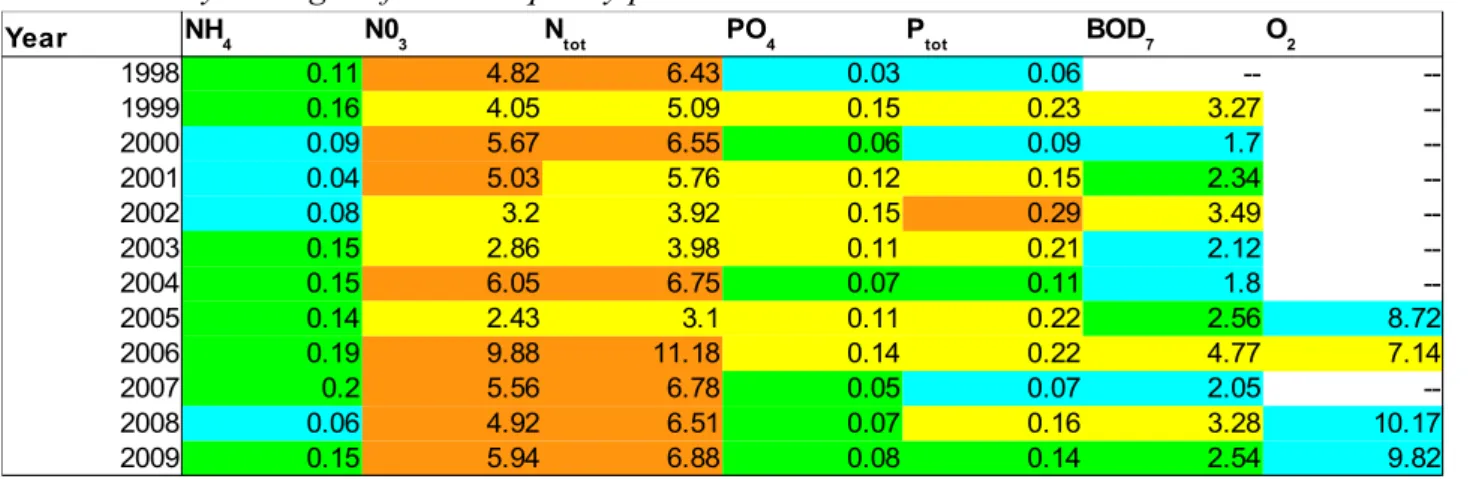
The monitoring data of land use, catchment borders, location of reaches, flow and water monitoring data were obtained from the WMI's reports “The Analysis of Land Use, Chemical Composition of Water and Precipitation in Typical Agro-ecosystems of Middle and West Picture 3: Location of the Graisupis river catchment (all the maps presented in this work apply Lithuanian Coordinate System (LKS-94)).
Lithuania”. These reports are issued annually since 1997 for the LEPA. They supply the monitoring results of typical agricultural catchments for the purpose of gaining needed knowledge for the calculation of nutrient loads from agricultural lands. Monthly values of water hydro-chemical parameters for the period of 1998-2009 have been used to prepare an observation file for the SWAT model calibration and validation. Daily discharge from the catchment data for the period of 2000-2009 were used for the calibration and validation of hydrology. The meteorological data were obtained from the LHMS. 21 years of time series were requested from the LHMS for hourly temperature, precipitation, relative humidity, temperature dew point, solar radiation and wind speed. Most of the data were collected in the Dotnuva meteorological station (located 4 km to the North from the Graisupis river catchment), except for the solar radiation data, which were collected in the Kaunas meteorological station (located 47 km to the South from the Graisupis river catchment). There were no solar radiation measurements in the Dotnuva meteorological station. Only daily averages for temperature and wind speed have been obtained from year 1988 to 1993. Hourly data (every three hours) were obtained for the period of years of from 1993 to 2008. Daily average of relative humidity and temperature dew point data were obtained from 02/1992. Hourly data (for every three hours) for relative humidity was available from year 1993 and for temperature dew point from 12/1993. Precipitation was available as daily cumulative samples from 1988 to 2007, and as hourly (for every six hours) samples from 2007. Solar radiation data were obtained from year 1998 to 2008. Daily minimal and maximal temperature, precipitation, wind speed, relative humidity and solar radiation were used as input of weather data time series for the SWAT model.
All inputs to the model for the weather time series should be of the same length. The time period chosen for the model input was 1988-2008. Solar radiation and relative humidity were not as long. Therefore, the value of -99 was used for the input from year 1988 until the measurements started. The value of -99 calls the weather generator module within the SWAT model. The weather generator uses statistical data obtained from weather measurements to generate the missing weather data. Temperature data for the SWAT until 1993 were estimated from the relationship obtained from hourly temperature data for the period of 1993-2008 (see Picture 4 and Picture 5). As the determination coefficients for both equations were high enough (more than 0.94), the estimation method was assumed good enough to provide the needed data.
Picture 4: Relationship between minimal daily temperature and average daily temperature.
-30 -20 -10 0 10 20 30 -40 -30 -20 -10 0 10 20 30 f(x) = 0.88x - 2.72
R² = 0.94 Minimal daily temperature versus
average daily temperature Linear Regression for Minimal daily temperature versus average daily temperature
Average daily temperature (in Celsius scale)
M in im a l d a ily te m p e ra tu re (i n C e ls iu s s ca le )
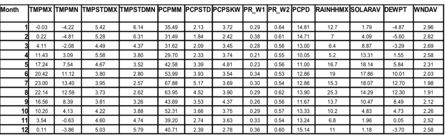
Statistical data for the weather generator were prepared using the same weather monitoring data described in the section above. Average or mean daily maximum air temperature for month (TMPMX) expressed in degrees of Celsius, average or mean daily minimum air temperature for month (TMPMN) expressed in degrees of Celsius, standard deviation for daily maximum air temperature in month (TMPSTDMX) expressed in degrees of Celsius and standard deviation for daily minimum air temperature in month (TMPSTDMN) expressed in degrees of Celsius were calculated using the maximum and the minimum daily temperature data8. Average or mean total monthly precipitation (PCPMM) expressed in mm H2O, standard deviation for daily precipitation in month (PCPSTD) expressed in mm H2O per day, skew coefficient for daily precipitation in month (PCPSKW), probability of a wet day following a dry day in the month (PR_W1), probability of wet day following a wet day in the month (PR_W2) and average number of days of precipitation in month (PCPD) were calculated from the precipitation data time series by using the pcpSWAT program, which was prepared by Stefan Liersch (http://www.brc.tamus.edu/swat/pcpSTAT.zip). Maximum 0.5 hour rainfall in entire period of record for month (RAINHHMX) expressed in mm H2O was the only one parameter, which was impossible to obtain or calculate from the available meteorological data. An assumption was made that the maximum 0.5 hour rainfall for the entire period of record for each month is more or less equal to the six hour cumulative rainfall sample for the period of 2007-2008. Average daily solar radiation for month (SOLARAV) expressed in MJ/m2/day, average daily dew point temperature in month (DEWPT) expressed in degrees of Celsius and average daily wind speed in month (WNDAV) expressed in meters per second were calculated from daily average values obtained from the LHMS. All statistical parameters are presented in Table 2.
8 Part of data 1988-1993 were estimated from statistical relationship with average data.
Picture 5: Relationship between maximal daily temperature and average daily temperature.
-30 -20 -10 0 10 20 30 -30 -20 -10 0 10 20 30 40 f(x) = 1.11x + 2.62 R² = 0.97
Maximal daily temperature versus average daily temperature
Linear Regression for Maximal daily temperature versus average daily temperature
Average daily temperature (in Celsius scale)
M a xi m a l d a ily te m p e ra tu re (i n C e ls iu s s ca le )
Two soil databases were obtained from the LEPA to prepare input for the SWAT model. The main database used for input was prepared by the National Land Service under the Ministry of Agriculture of the Republic of Lithuania. The scale of this GIS vector database is 1:10000. Another soil database of scale 1:300000 was used in the places where a more detailed GIS database lacked cover (mostly in areas covered by forests). The national soil classification system was linked to the Food and Agriculture Organization (FAO) soil classification. By linking it to the FAO system it was possible to get soil parameters from soil databases, which were prepared for the world. The Harmonized World Soil Database (HWSD) (Fischer et al., 2008) was used to obtain most of the soil parameters. Other parameters were estimated, left default or obtained through calibration. The estimation of soil parameters is explained in the next section. The prepared soil layer is presented in c part of Picture 6.
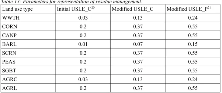
Land use in the Graisupis river catchment is monitored yearly by the WMI. Land use of 2008 was used as input for the model (see d part of Picture 6). This was due to the availability of data at the beginning of the model preparation. The most appropriate parameter compositions were assigned to land use categories from the prepared crop and urban SWAT databases through a look-up table. The assigned categories are presented below in Table 3.
Table 3: Assigned land use from SWAT database comparing to original land use. Original land use Assigned land use from crop or urban
databases Code of assigned land use
Homestead Residential-Low Density URLD
Winter wheat Winter Wheat WWHT
Pastures Pastures PAST
Summer wheat Corn CORN
Water Water WATR
Canola Spring Canola-Polish CANP
Barley Spring Barley BARL
Forest Forest-Deciduous FRSD
Maize Sweet corn SCRN
Vegetable garden Garden or Canning Peas PEAS
Sugarbeet Sugarbeet SGBT
Farm facilities Industrial UIDU
Other crops Agricultural Land-Close-grown AGRC
Other agricultural areas Agricultural Land-Generic AGRL Table 2: Statistical parameters for the weather generator.
Month TMPMX TMPMN TMPSTDMX TMPSTDMN PCPMM PCPSTD PCPSKW PR_W1 PR_W2 PCPD RAINHHMX SOLARAV DEWPT WNDAV
1 -0.03 -4.22 5.42 6.14 35.49 2.13 3.72 0.29 0.64 14.81 12.7 1.79 -4.87 2.96 2 0.22 -4.81 5.28 6.31 31.49 1.84 2.42 0.38 0.61 14.71 7 4.09 -5.60 2.82 3 4.11 -2.08 4.49 4.37 31.62 2.09 3.45 0.28 0.56 13.00 6.4 8.87 -3.29 2.69 4 11.43 3.09 5.58 3.80 29.70 2.33 3.74 0.21 0.55 10.05 5.2 13.31 1.55 2.58 5 17.24 7.54 4.67 3.52 42.58 3.39 4.81 0.23 0.56 11.00 16.7 18.14 5.84 2.31 6 20.42 11.12 3.80 2.80 53.99 3.93 3.54 0.34 0.53 12.86 19 17.86 10.01 2.03 7 23.00 13.40 3.95 2.57 67.88 5.17 3.69 0.30 0.54 12.86 15.3 18.07 12.70 1.98 8 22.14 12.59 3.73 2.62 63.95 4.52 3.90 0.29 0.62 13.90 25.3 14.29 12.30 1.91 9 16.56 8.39 3.81 3.26 43.69 3.53 4.37 0.26 0.56 11.67 13.7 10.47 8.49 2.12 10 10.20 4.13 4.22 3.88 52.31 3.66 3.75 0.29 0.57 13.33 10.2 4.83 4.73 2.26 11 3.54 -0.63 4.60 4.74 39.20 2.74 3.63 0.33 0.54 13.24 6.8 1.96 0.05 2.52 12 0.11 -3.86 5.03 5.79 40.71 2.39 2.78 0.36 0.60 15.14 11 1.18 -3.70 2.58
Slopes were obtained by using slope definition module in ArcSWAT. 3 categories have been chosen: from 0 to 1 %, from 1 to 3 % and slopes more than 3 % slopes. The distribution of slopes is presented in part b of Picture 6.
5.3.2 Estimation of Soil Parameters
The obtained GIS soil database had very few (in most cases none) usable parameters for the model input. Usable data were the soil classification according to the national soil classification system, which was related to the FOA soil classification system. Overall 12 soil types were present in the Graisupis river catchment (Appendix, Table 1). These data were obtained from the soil GIS layer attributes. Soil parameters were mainly obtained from HWSD. Some parameters were estimated or left default. The SWAT model requires defining some parameters for the whole soil profile as well as for each layer in the soil profile. In the HWSD, the soil profile is divided into two soil layers: 0 to 30 cm and 30 cm to 100 cm. Therefore, the number of layers (LAYERS) for all soils was set to 2. The soil hydrological group (HYDGRP) was estimated using the USDA proposed classification, which is based on soil textures (such as sand, loam sand, heavy clay, etc, which were available in the HWSD). The maximum rooting depth of the soil profile (SOL_ZMX) was set to 1000 mm (as the overall depth of the soil profile) with the exception of Calcaric Arenosols, which was set to 700 mm because in the HWSD the obstacles to roots were set to 60-80 cm. The parameters for the fraction of porosity (void space) from which anions are excluded (ANION_EXCL) and the potential or the maximum crack volume of the soil profile expressed as a Picture 6: Elevation (a), slope (b), soil (c) and land use (d) data for the Graisupis river catchment.
fraction of the soil volume (SOL_CRK) were left default at 0.5. These parameters are optional and the model proposed value (if no data is entered) is 0.5. The depth from the soil surface to the bottom of layer (SOL_Z), moist bulk density (SOL_BD), available water capacity (SOL_AWC), organic carbon content (SOL_CBN), clay content (CLAY), silt content (SILT), sand content (SAND), rock content (ROCK) and electrical conductivity (SOL_EC) were taken from the HWSD. Available water capacity was available just for all soil profile. Thus, an assumption was made that it is the same for both soil layers. Saturated hydraulic conductivity (SOL_K) (mm/hr) was calculated using Equation 1, which was developed by assessing the relationship between parameters in the prepared SWAT soil database. The strength of statistical relationship was R2=0.76 between the values estimated by this equation and the real values.
Equation 1: Formula for calculation of saturated hydraulic conductivity.
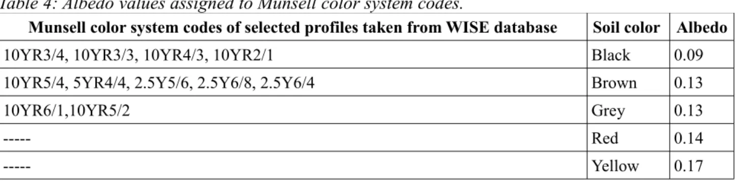
Moist soil albedo (SOL_ALB) was not available in the HWSD. It was estimated by using the colors of layers in the soil profile. Color codes in the Munsell color system for different types of soils were available in ISRIC-WISE Harmonized Global Soil Profile Dataset (Batjes, 2008). Soil profiles of the soil types existing in the Graisupis river catchment (and which are in Lithuania or closest to Lithuania) were selected for obtaining the colors of soil layers. Albedo was estimated by using the relationship between the (moist) soil color of the topsoil and the soil albedo given in the article of Gisjman et al. (2007). Color codes were related to the names of colors by using visual senses with the aid of website http://www.it.lut.fi/research/color/demonstration/demontration.html. The final result is presented in Table 4.
Table 4: Albedo values assigned to Munsell color system codes.
Munsell color system codes of selected profiles taken from WISE database Soil color Albedo
10YR3/4, 10YR3/3, 10YR4/3, 10YR2/1 Black 0.09
10YR5/4, 5YR4/4, 2.5Y5/6, 2.5Y6/8, 2.5Y6/4 Brown 0.13
10YR6/1,10YR5/2 Grey 0.13
--- Red 0.14
--- Yellow 0.17
The USLE equation soil erodibility factor (USLE_K) was estimated using the Williams equation given in the SWAT Input/Output File Documentation (Neitsch et al. 2004). This equation requires sand, silt, clay and organic content parameters. All soil parameters used in the model are presented in Appendix A.
5.3.3 Data Adjustments
After studying the SWAT technical documentation some problems were identified with the input data. The first was that the precipitation data might be incorrect due to the effects of rain gauges, which were not designed to shield wind effects. The design of rain gauges has been confirmed by Natalija Gaurilcikiene, the LHMS responsible person for the Dotvuna meteorologic station. It has
K
s=
1.7499
×
e
0.0751×SAND
1000
×
e
−0.211×CLAYbeen confirmed that the Dotvuna meteorological station uses only simple rain gauges, which are not designed to shield wind effects. According to Larson and Peck cited in the SWAT documentation for these types of rain gauges the deficiencies of 10% for rain and 30% for snow are common (SWAT technical documentation). Therefore, all precipitation data were changed based on this information. For days when there average temperatures were above 0 degrees of Celsius, the precipitation was increased by 10%, and for days when temperature was equal to or below 0 degrees of Celsius, the precipitation was increased by 30%.
Another problem with the input data was connected with wind speed measurements. According to the SWAT technical documentation, “SWAT assumes wind speed information is collected from gauges positioned 1.7 meters above the ground surface” (Neitsch, et al., 2005). However, wind speed measurements are done at 10 meters above the ground in the Dotnuva meteorological station. Therefore, a transformation was done with Equation 2 to obtain input required by the SWAT model. This equation has been approved and recommended by the LHMS (Smitiene, 2007).
Equation 2: Formula for recalculation of wind data (wind shear exponent is equal to 0.25).
5.4 Model Preparation
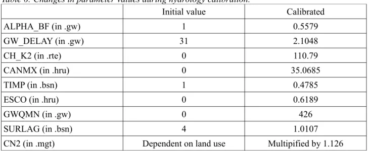
Model preparation was made by putting in the data and parameters into the right formats and databases, setting up the SWAT model with the use of SWAT modules and then calibrating and validating the prepared model. Calibration was the most prolonged faze. It was made with the help of the SWAT-CUP 2.1.5 program.
5.4.1 Dividing the Catchment
The SWAT model is a semi-distributed parameters model. Pollutant loads originating anywhere in a sub-basin are treated equally. Thus, it is better to divide the basin into smaller sub-basins to represent the spatial variability of physical conditions in a watershed. Moreover, shortcomings of the SWAT model for overland pollutant routing are reduced if more or all physically meaningful sub-basins are used.
For this study the Graisupis river catchment was divided into 9 basins. For each of this sub-basin separate reach segment was assigned. The division of the catchment is presented in Picture 7.
For the watershed delineation the real boundaries of the catchment was used, which were obtained from the WMI report of 2009. The location of reaches was also obtained from the same report. The boundaries of the catchment were used as a mask and the reaches were burned into DEM with the watershed delineation module of ArcSWAT software. For DEM based stream definition an 80 ha area was chosen. With the mentioned settings the watershed delineation module of ArcSWAT software divided the whole catchment into 9 sub-basins. To align the external boundaries of these sub-basins with the real catchment boundary, the sub-basin layer was edited manually. Stream definition was made with the pre-defined watershed and stream datasets in order to set up the final watershed configuration.
V
1.7m=
V
10m×
41.7
5.4.2 Calibration of Flow
For the calibration of water flow, daily data for the Graisupis river flow were available from year 2000. Monthly data for river flow were available from year 1998. The period from 2000 to 2006 was used for calibration. For validation purposes the data from year 2007-2009 were used. The split between calibration (7 years for calibration) and validation (3 years for validation) years was based on the common practices observed in scientific literature. For nitrate calibration monthly data from 1998 was available. Yet, calibration and validation of nitrate loads were made on the same periods as that water flow. The data of 1998-1999 were left out due to the lack of daily water flow values. The watershed model performance criteria were based on the article of Moriasi et al. (2007) (see Table 5 on the next page). The least aim for calibration was to reach a good performance rating. It was intended to use only monthly values in later steps. Thus, the statistics for a monthly time step were used.
The warm-up (or spin-up period as it is used in some literature sources) period of 3 years was selected for hydrology calibration and validation. For nitrates this period was 5 years. The length of warm-up periods was based on the time necessary to eliminate the effects of initial model values on final results. Several runs were performed with different warm-up periods. Those, which indicated the best effect on model performance increase, were selected.