Latent space models for multidimensional network data

(1)

Sapienza, University of Rome

Department of Statistical Sciences Ph.D. in Methodological Statistics

Latent space models

for multidimensional network data

Candidate: Silvia D’Angelo Thesis advisor: Prof. Marco Alf`o

(2)

(3)

(4)

(5)

Pizza brought me so far, but does not get all the credits.

During my master’s degree, Alessandra, Valentina, Giulia and Alessia made my stay at the fourth floor so nice that me and Tullia decided not to leave for another three years. In all these years of friendship, they still have not understood why we did it. These last years would not have been the same without Tullia, Carlo and Marco. We have shared a lot, especially Stanza 41. This room taught us much about coexistence and helped us becoming friends. With them, Lampros, Riccardo, Francesca, Julianne, Brendan and all the others, from Rome to Dublin, contributed making PhD life a great adventure. My experience could have not been the same without Marco, who let me work freely, and never neglected me. There is much in life outside Statistics and I am happy to have found a supervisor who stands by that.

Laura, Elena, Giorgia and Caterina, friends of a lifetime, accompanied me through this PhD, as they did with all other episodes in my life before this one and will do with next to come.

This thesis is dedicated to my parents, Antonietta and Paolo, for giving me an inspiring life and for all the journeys we made together. You always wanted what was best for me, and met me halfway all the times our definitions of best did not match. Alessandro, my brother, this thesis is also for you, for turning the volume so loud while playing videogames that even people in Ariccia could hear you and for caring so much about me to come and visit me in Dublin, even though is Dublin. Last, this is for you Michael, and for us. We know why.

(6)

(7)

vii

List of Figures

1.1 Graphical example of asymmetrical binary network, with 4 nodes and

5 edges. . . 4

1.2 Graphical example of an asymmetrical binary multidimensional net-work, with 4 nodes and 3 views. . . 5

1.3 Two examples of a latent space representation of a network. . . 10

2.1 Latent space representations of a network with 3 nodes. . . 21

2.2 Hierarchy structure of the model. . . 24

2.3 Eurovision data: some exploratory statistics. . . 29

2.4 Covariates. . . 30

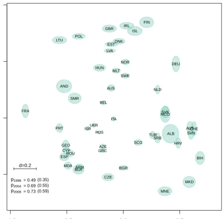
2.5 Estimated latent positions 1998-2015. The legend reports the proba-bilities corresponding to a distance of 0.2 in the latent space, years 1998, 2004 and 2008. The values refer to the case ofx2,ij = 0, within the brackets are reported the values for x2,ij = 1. . . 34

2.6 Estimated distances between couple of countries, 1998-2015. . . 35

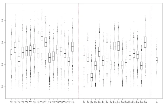
2.7 Boxplots for model parameter estimates and the coefficient for X2, 1998-2015. . . 35

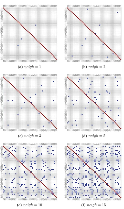
2.8 Intersections of the set of neighbours LNi,r and GNi,r, 1998-2015 . . 36

2.9 Intersection of the set of neighbours LNi,r∗ i and CNi,r∗i, 1998-2015. On the left column, in brackets, are reported the values of r_i∗. . . 37

3.2 Synthetic representation of the heuristic procedure for model selection. The thresholds have been fixed via a cross validation exercise and are: 1= 0.12, 2 = 0.2,c1 = 0.5,c2 = 0.8, respectively. . . 52

3.3 Fruit multiplex: Pairplots of the observed out- and in-degrees of the networks. The upper diagonal matrix represents the associations between the observed out-degrees in any couple of networks, while the lower diagonal refers to the association between the in-degrees. The values of the Spearman correlation indexes are reported. . . 56

3.4 Fruit multiplex. Estimated latent coordinates for the countries. The segments represented at the bottom of the plot displays the value for the first quartile of the estimated distribution of the distances. . . . 57

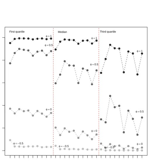
3.5 Fruit networks. Estimated probabilities in the multiplex, for different values of the estimated distances ( first quartile, median and third quartile) and of the φ(_ijk) coefficients. . . 58

(11)

List of Figures xi

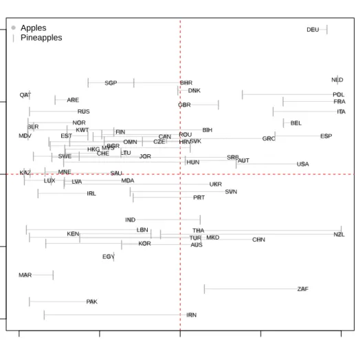
3.6 Apples (black) and Pineapples (grey) networks. Estimated sender

and receiver effects of the countries. . . 59

4.2 Scenario I. (Mean) estimated posterior distribution for the number of clusters G. . . 76

4.3 Scenario II. (Mean) estimated posterior distribution of the number for clusters G. . . 77

4.4 Scenario III. (Mean) estimated posterior distribution for the number of clusters G. . . 78

4.5 Scenario IV. (Mean) estimated posterior distribution of the number for clusters G. . . 79

4.6 Vickers data. Adjacency matrices for the three networks. . . 80

4.7 Vickers data. Posterior distributions of the number of clusters. . . . 83

4.8 Vickers data. Average co-occurrence of the nodes in the same cluster and estimated cluster labels. . . 83

4.9 Vickers data. Posterior distributions of component means and esti-mated latent coordinates. In the right plot, triangles indicate female students, while dots correspond to male students. . . 84

A.1 Eurovision data: boxplots for the estimates of the logistic parameters, periods 1998-2007 and 2008-2015. . . 97

A.2 Eurovision data: estimated latent positions, periods 1998-2007 and 2008-2015. . . 98

A.3 Eurovision data: estimated distances between couple of countries for the period 1998-2007. . . 99

A.5 Eurovision data: intersections of the set of neighbours LNi,r and GNi,r, for the period 1998-2007. . . 101

A.7 Eurovision data: intersections of the set of neighbours LNi,r and GNi,r, for the period 2008-2015. . . 103

A.8 Simulations: first scenario. . . 105

A.9 Simulations: second scenario. . . 107

A.10 Simulations: third scenario. . . 109

A.11 Simulations: fourth scenario, multiplex withn= 50 and K= 10. Es-timated averages and standard deviations for the network parameters. 110 A.12 Simulations: fourth scenario, multiplex with n = 50 and K = 20. Estimated averages and standard deviations for the network parameters.111 A.13 Simulations: fourth scenario, multiplex with n = 50 and K = 30. Estimated averages and standard deviations for the network parameters.111 B.1 Boxplots of the estimated posterior distributions for the intercept parameters α(k). Red dots indicate the true, simulated, values of the intercepts. . . 121

(12)

B.2 Boxplots of the estimated posterior distributions for the coefficient

parametersβ(k). Red dots indicate the true, simulated, values of the

coefficients. . . 122

D.1 Hierarchy structure of our formulation of the lsjm model. . . 132

List of Tables

2.1 DIC values for fitted models. . . 32

2.2 Model parameters: estimated averages and standard deviations,

1998-2015. . . 32

2.3 Average and maximum number of intersections of the set of the closest

latent positions and the closest geographical positions. . . 34

3.1 The class of models defined by the different assumptions on the

sender/receiver effects. . . 44

3.2 Simulation study. Spearman correlation between the simulated and the estimated sender effects, by simulation scenario and true model

structure. . . 49

3.3 Simulation study. Spearman correlation index between the simulated

and the estimated receiver effects. . . 49

3.4 Simulation study. Distance correlation between the simulated and the

estimated edge-probabilities. Last column (P C) shows the Procrustes

correlation between the simulated and the estimated latent space

coordinates. . . 50

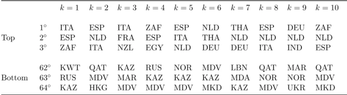
3.5 Estimated sender effects: top and bottom three exporting countries. 55

3.6 Estimated receiver effects: top and bottom six importers countries. 55

3.7 Averages and standard deviations of the estimated posterior distri-butions for the intercept and the scale coefficient parameters in the

fruit networks. . . 55

4.1 Scenario I. Procrustes correlation between estimated and simulated latent spaces and Adjusted Rand Index for the estimated-simulated

cluster labels. . . 75

4.2 Scenario II. Procrustes correlation between estimated and simulated latent spaces and Adjusted Rand Index for the estimated-simulated

(13)

List of Tables xiii

4.3 Scenario III. Procrustes correlation between estimated and simulated latent spaces and Adjusted Rand Index for the estimated-simulated

4.4 Scenario IV. Procrustes correlation between estimated and simulated latent spaces and Adjusted Rand Index for the estimated-simulated

4.5 Vickers data. Average estimated edge probabilities within and between

clusters. . . 84

A.1 Eurovision data: country ISO3 codes. . . 96

A.2 Eurovision data: estimated averages and standard deviations for the

network parameters in the multiplex 1998-2007. . . 97

A.3 Eurovision data: estimated averages and standard deviations for the

network parameters in the multiplex 2008-2015. . . 97

A.4 Simulated values for the intercept and the coefficient terms in the

multidimensional networks considered in scenarios I-III. . . 104

A.5 Multivariate Gaussian latent coordinates. Averages for the estimated logistic parameters and the procrustes correlation between true and

estimated latent spaces. . . 104

A.6 Multivariate Gaussian latent coordinates. Standard deviations for the estimated logistic parameters and the procrustes correlation between

true and estimated latent spaces. . . 104

A.7 Mixture of multivariate Gaussian distributions latent coordinates. Averages for the estimated logistic parameters and the procrustes

correlation between true and estimated latent spaces. . . 106

A.8 Mixture of multivariate Gaussian distributions latent coordinates. Standard deviations for the estimated logistic parameters and the

procrustes correlation between true and estimated latent spaces. . . 106

A.9 Hotelling T squared latent coordinates. Averages for the estimated logistic parameters and the procrustes correlation between true and

estimated latent spaces. . . 108

A.10 Hotelling T squared latent latent coordinates. Standard deviations for the estimated logistic parameters and the procrustes correlation

between true and estimated latent spaces. . . 108

A.11 Simulations: fourth scenario. Procrustes correlation. . . 110

A.12 Results of the comparison with thelsjmmodel. Averages and standard

deviations for the estimated intercepts and the procrustes correlation

between true and estimated latent spaces. The acronym lsmmn is

used to indicate the model presented in this work. . . 112

B.1 Fao data: country ISO3 codes. . . 115

B.2 Block II,n= 50, K= 10. Percentage of time each model is selected

by the Heuristic search. . . 123

B.3 Block II,n= 65, K= 10. Percentage of time each model is selected

(14)

D.1 Simulated multiplex withn= 25 andK = 3. Mean and standard

devi-ations of the Procrustes correldevi-ations between simulated and estimated

latent spaces, according to the three different approaches. . . 135

D.4 Simulated multiplex with n = 100 and K = 5. Mean and

stan-dard deviations of the Procrustes correlations between simulated and

(15)

xv

Abstract

Network data are any relational data recorded among a group of individuals, the nodes. When multiple relations are recorded among the same set of nodes, a more complex object arises, which we refer to as “multidimensional network”, or “multiplex”, where different relations corresponding to different networks.

In the past, statistical analysis of networks has mainly focused on single-relation network data, referring to a single relation of interest. Only in recent years statistical models specifically tailored for multiplex data begun to be developed. In this context, only a few works have been introduced in the literature with the aim at extending the latent space modeling framework to multiplex data. Such framework postulates

that nodes may be characterized by latent positions in a p-dimensional Euclidean

space and that the presence/absence of an edge between any two nodes depends on such positions. When considering multidimensional network data, latent space models can help capture the associations between the nodes and summarize the observed structure in the different networks composing a multiplex.

This dissertation discusses some latent space models for multidimensional network data, to account for different features that observed multiplex data may present. A first proposal allows to jointly represent the different networks into a single latent space, so that average similarities between the nodes may be captured as proximities in such space. A second work introduces a class of latent space models with node-specific effects, in order to deal with different degrees of heterogeneity within and between networks in multiplex data, corresponding to different types of node-specific behaviours. A third work addresses the issue of clustering of the nodes in the latent space, a frequently observed feature in many real world network and multidimensional network data. Here, clusters of nodes in the latent space correspond to communities of nodes in the multiplex.

The proposed models are illustrated both via simulation studies and real world applications, to study their perfomances and abilities.

Acknowledgments

A special thank goes to the reviewers, Veronica Vinciotti and Giuliano Galimberti, for their precious comments and feedback.

(16)

(17)

1

Chapter 1

Introduction

In the last decades, statisticians showed an increasing interest raised in the analysis of network data, and a large variety of models has been developed for this task. In the beginning, network analysis was deeply linked with social network analysis, as first network data were collected and analysed by quantitative social scientists (Jacob Moreno and Helen Jennings, 1930). Nowadays, network data come from many other different fields: biology, telecommunications, economic and behavioural sciences, and so on. While first models focused mainly on studying global network properties and network summary statistics behaviour, more recent ones have also migrated to the analysis of single relationships. Indeed, many modelling techniques have been proposed: from visualization to link prediction, a lot of different approaches have been developed. In particular, recent developments in network analysis focused on feasible representations of the complex dependency structure present in network data, by means of latent variables. Also, in the last years statisticians started to focus on more complex types of network data, as for example networks arising from different measurements or measurements repeated trough time on the same sample of units. Such data are called multidimensional network data, and their study is a flourishing area in network analysis.

The purpose of this chapter is to introduce the reader to the main concepts in network analysis and, in particular, in latent variable models for network data. First, basic notation that will be used throughout the dissertation will be introduced, together with a description of some well known and widely used exploratory and summary statistics to characterize observed networks. Then, we will introduce some of the first approaches proposed in the literature to network data, that have paved the way to modern network analysis. Last, we will discuss latent space models for network data, their principal forms and main assumptions. The final part of this chapter will give a brief summary of the dissertation structure.

1.1 Single and multidimensional networks

Any relational data observed for a group of units form a network. As networks can be represented by means of graph theory, units in the data are often referred to as nodes. Any relation that exists between any two nodes is represented by anedge

(18)

as the realization of a random graphG:

G= (V, E),

where V is the set of the nodes and E that of the edges. We will denote the

cardinality of V byn, which is the number of nodes, indexed by i, j= 1, . . . , n. A

general edge may be denoted byeij.

Depending on the type of relation being recorded, the set of edges may be charac-terized in different ways. One major distinction is whether the edges are valued or not:

• Binary edges appear when the relation that is being measured can either

be present or not. Therefore, an edge is present between two nodes if the relation is present, otherwise it is not. A typical example of binary edges could be that of a network where a group of people, the nodes, are asked to state whether or not they consider other units in the sample as friend; a declaration of friendship would correspond to an edge. A network having binary edges

is calledbinary network and may be represented via an adjacency matrixY,

with dimension n×nand general element

yi,j =

(

1 if an edge exists between nodei andj,

0 else.

• Weighted edges, instead, arise when the relation being recorded is valued.

In this context, what is of interest is the strength of the relation between the nodes, represented by the values associated with the edges. Depending on what is being measured, the weights may be discrete or continuous, positive, negative or both. A typical example would be that of telephone networks. Suppose that, for the same group of people in the previous example, we recorded the number of calls between any two of them in a given period of time. Here, the strength of the relation between two nodes is represented by the number of

phone calls they made: the higher, the grater. Of course, if a dyad (i, j) does

not have any phone call, the weight associated with the corresponding edge is

0. A network with weighted edges is calledweighted network.

The presence of an edge between a dyad (a couple of nodes), or the potential weight associated with it, does not tell the whole story. Indeed, it may be relevant to

check whether the presence of an edge between nodes (i, j) is accompanied with the

presence of an edge between (j, i). Indeed, edges may have a direction, as not all

relations are reciprocal, and we can distinguish them in:

• Undirectededges, when the relation is reciprocal. For example, if one was

recording kinships among a group of people in a village, the fact that personi

is related withj implies that also j is related withi. This reciprocity is called

symmetry and network exhibiting such characteristic are called symmetric

networks.

Similar to symmetry is thereflexivity property. This indicates a node that

(19)

1.1 Single and multidimensional networks 3

associated with eii in weighted networks. Such a property may be observed in

some biological networks, for example in protein-protein interaction networks, but is quite rare in social network data.

• Directed edges represent relations which potentially have a direction. For

example, a friendship network may have directed edges, as the fact that nodei

thinks that j is a friend does not imply the opposite. A network with directed

edges is called asymmetrical.

For asymmetrical networks, it may be of interest to consider the number of

mutual edges between dyads, that is P

i<jyijyji. The presence of an high

quantity of mutual links in asymmetrical networks would denote that most of the dyads exhibit some reciprocity, on the opposite, a low mutuality would denote a low value, or the absence, of reciprocity.

From this moment on, in this introduction, we will focus on binary networks, as the present thesis develops model for such type of network data. For a richer review of

weighted networks, see for example Wasserman and Faust, 1994.

Note that, potentially, a network with nnodes may have a maximum number of

edges equal to n2, if the network isreflexive, or a maximum ofn(n−1) edges if it is

not. A non-reflexive network can be either ( denseorcomplete if Pn i=1 Pn j≤iyij =n(n−1), sparse if Pn i=1 Pn j≤iyij < n(n−1).

However, complete networks are quite hard to encounter in practice and, therefore, are usually of low interest. In general, a binary network may be called dense if almost all the entries of the corresponding adjacency matrix are 1 and sparse when,

on the opposite, almost all of them are 0. An index of sparsity is the density, which

computes the ratio between the number of observed edges and the maximum possible number of edges in a network; values of this index close to 0 denote sparsity, while values close to 1 indicate a dense network.

At a more local level, the number of edges corresponding to each node is a first indicator of how nodes interact with each other; this behaviour may be captured by

looking at the nodes’sdegree. The degree d(i) of nodeibasically counts how many

edges are incident with it. In symmetric networks, it may be defined equivalently

either looking at the columns or at the rows of the network adjacency matrix Y:

d(i) = n X j=1 yij = n X j=1 yji.

Instead, in asymmetric matrix, rows and columns convey different informations regarding the behaviour of a node. By convention, we will state that a given row

i collects edges going out of node i, edges that node iis sending, while columni

collects edges entering node i, which the node is receiving. Then, we might define

the out-degree dout(i) and the in-degree din(i) of nodeias:

dout(i) = n X j=1 yij, din(i) = n X j=1 yji.

(20)

Different network data may have different degree distributions din(i), dout(i),

i= 1, . . . , n, which can be used to characterize the network. For example, some

networks may have homogeneous degree distributions, with all degrees having similar values. Other networks may have a small group of nodes with an high degree and the rest with only a few connections.

a c

d b

Figure 1.1. Graphical example of asymmetrical binary network, with 4 nodes and 5 edges.

Figure1.1provides an example of a network, which has n= 4 nodes and 6 directed

edges. In this example, the in-degrees and out-degrees distributions are mostly

inho-mogeneous, withdout(a) = 3, dout(b) = 2,dout(c) = 1, dout(d) = 0 anddin(a) = 0,

din(b) = 1, din(c) = 2, din(d) = 3. Node a is the most active of the 4, with an

out-degree of 3, but it is not popular at all, as the in-degree is null. The concepts of

popularity and ofactivity, referred to the propensity of nodes to receive/send many

links, will be further discussed in the next section and in Chapter 2, as a way to

characterize the individual nodes behaviours.

Notice that one may not only look at dyadic relations, but at higher order ones as well; triangles, for example, are configurations arising when a group of three

nodes (i, j, l) are all interacting with one another. The number and position of

the edges may also be used to define other summary statistics, as for example

centrality statistics, denoting the importance of each node in a network, in terms

of its relevance in determining the observed structure. For different definitions of centrality, network statistics and other basic characterization of network data we

refer to Salter-Townshend et al.,2012and Wasserman and Faust, 1994.

1.1.1 Multidimensional networks

The type of network data we have defined in the previous section is the most simple one, where a single relation is recorded among a same group of nodes. However, sometimes it may be the case that multiple relations are recorded among the same

group of nodes. Then, the corresponding network is referred to asmultidimensional

network ormultiplex. A binary multidimensional network may be represented by

a collection of adjacency matrices Y={Y(1), . . . ,Y(K)}, withk= 1, . . . , K. The

index k denotes the kth relation recorded on then nodes, represented by the kth

network, or view. Thekth adjacency matrix has general entry

y_i,j(k) =

(

1 if an edge exists between nodei andj in the kth network,

(21)

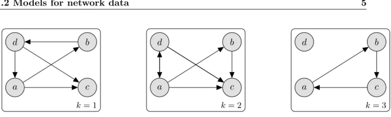
1.2 Models for network data 5 a c d b a c d b a c d b k= 1 k= 2 k= 3

Figure 1.2. Graphical example of an asymmetrical binary multidimensional network, with 4 nodes and 3 views.

The summary statistics defined in the previous section for single network data may be computed for the views of a multiplex as well. Also, the same characterization in

terms of types of edges and relations, binary, weighted, etc., still holds. Figure1.2

represents, as an example, an asymmetrical binary multidimensional network, with 4 nodes and 3 views. These 3 networks could correspond, for example, to data collected

among 4 people working together, who were asked whether they were friends (k= 1),

if they worked well together (k= 2) and if they considered another person reliable

(k= 3). As it can be seen from the picture, different relations correspond to different

configurations in the views. Thus, multidimensional networks convey a variable information regarding the nodes of interest. The different views, when analysed all together, may bring interesting insights on the relational structure among the nodes, not captured by the analyses of the single networks alone. Indeed, in the previous

example, if the research question was how do the co-workers interact?, considering

jointly the different relations would give a richer picture on the interactions. Also, when the number of observed networks increases, analysing the multiplex as a single

object may be a more parsimonious approach, when compared to K separate single

network analyses.

A particular case of multidimensional network is represented bydynamic networks,

which are defined by the recording of the same relation trough time, over the same set of nodes. One example could be that of a class of students, followed from the first year of studies until the last one, recording friendship relationships each year. As students spend more time together, new friendships may begin and old ones may end; analysing such an evolution may be of interest.

Until now, we have introduced some basics concepts and definitions regarding single and multidimensional network data. In the following section, we will discuss some of the main tasks arising when attempting to model such data. Further, we will briefly present the classical models developed for network data, their purposes, characteristics and limitations.

1.2 Models for network data

As mentioned before, network data record relations among a group of units, the nodes, and, for modelling purposes, an observed network may be assumed to

(22)

be the realization of a random graph. Hence, to better understand networks, one may aim at reconstructing the process that lead to their observed realizations. In

other words, one may aim at modelling the edge probabilitiespij underlying a given

network Y, that is, the probabilities of observing an edge between nodes (i, j),

i, j= 1, . . . , n. Do edges probabilities depend on the dyad or are they constant over

the whole network? Is there a node that has a higher probability than others to send links? What do these probabilities depend on? These questions, and many others, drove the definition of different stochastic models for network data, with different aims and hypotheses. As in other branches of statistics, there is no “true” model to analyse network data; the choice among competing models mainly depends on the purposes of the analysis, and, of course, the data at hand. A factor that may determine the choice of a particular model is its computational complexity. Network data are high dimensional by nature, as, for example, even a “small”, non

reflexive, network with “only”n= 50 nodes, has potentially 50(50−1) = 2450 edges;

the computational burden increases quadratically with the number of nodes, which sometimes makes complex models unfeasible. Also, with multidimensional networks the computational complexity is additionally increased by the extra dimension given by the number of views. On the other hand, another task arising with network data is that such complex objects may be the realisations of highly dependent random variables. Therefore, simple models may prove unable to represent network data, and more sophisticated representations should be considered. This trade-off between faithful representation and feasible estimation is a key issue when dealing with network data. Below, we will provide a synthetic summary of the main classes of models developed in network analysis to model edge probabilities and briefly discuss them. We may consider:

• Erdös-Rényi model. Proposed by the homonymous authors in 1959 (Erdős

and Rényi, 1959), this first model is the simplest of all, as it assumes

inde-pendent and constant edge probabilities across the network. Although its simplicity makes it computationally feasible to fit and various theoretical results regarding it are available, its over simplistic assumptions make it often inappropriate to describe real world network data. However the Erdös-Rényi model is still a reference model in network analysis and sometimes it may be useful to compare different representations from more complex models. • p1 model. Introduced by Holland and Leinhardt, 1981, this model still

assumes independence between edges, but removes the assumption of constant edge probabilities. Indeed, it postulates that edge probabilities are function of some summary statistics (number of nodes, out-/in-degrees and number of mutual links between dyads) and four types of parameters. Such parameters capture the base rate for edge probabilities, the sender/receiver propensities of

the nodes, and the level of mutuality in the network. Thep1model introduces

the concepts of sender/receiver propensities of the nodes, in this context denoted by productivity/attractiveness. Such characterizations have been later recovered and adapted in different other models, often proving to be quite useful to feasibly represent nodes individual behaviour in asymmetrical networks.

(23)

1.2 Models for network data 7

• p2 model. This model is an extension of the p1 model, proposed by Duijn,

Snijders, and Zijlstra,2004, where sender and receiver effects are modelled as

additive random effects and covariates may be included in the specification of the model for the edge probabilities. The inclusion of covariates is a relevant step forward in network analysis, as it allows to explain an observed network using node-specific external information, other than with the summary

statistics alone. Covariates account for homophily by attributes, that is, nodes

with similar attributes may be more likely to link. However, the selection of covariates relevant to the analysis may prove to be a difficult task; covariates alone may not be capable to capture the whole dependence structure underlying network data.

• p∗ model or ERGM (exponential Random Graph Models). This class of

models represent an extension of Markov Graphs, proposed by Frank and

Strauss, 1986, where it is assumed that possible edges between disjoint pairs

of nodes are assumed to be independent, conditional on the rest of the graph. Thus, Markov Graphs introduce the idea of conditional independence between the edges, overcoming the independence hypothesis of previous models. ERGM builds on Markov Graphs and postulate that edge probabilities are of an exponential family form, and are also parametric functions of some summary

statistics. A new feature ofp∗ models is based on the introduction of a number

of triangles statistic when modelling edge probabilities, as a way to account for transitivity. Transitivity is a characteristic of many real network data,

which may be expressed as “a friend of mine is a friend of mine”. Higher order statistics can be considered as well when modelling edge probabilities, increasing the complexity of the model. Some basic references can be found in

Wasserman and Pattison, 1996and Robins et al.,2006.

• Latent variable models.This class of models aim at explaining the observed

connections in a network by means of some unobserved, latent variable. In general, this broad class of models studies edge probabilities via an additional layer of modelling, that is the layer of the latent variable(s); edges are assumed to be independent conditional on some parametric function of the latent variable(s). As in Markov Graphs, the conditional independence assumption allows to better model the complex structure of network data, while the latent variable(s) introduces flexibility in the analysis. The two main sub-classes that have been proposed in the literature are:

– Stochastic Block models. This class of models is an extension of

blockmodelling, a non-stochastic approach for clustering of network data.

Block models assume that a network can be decomposed into a set ofG

clusters,C1, . . . , CG. Interactions within and between such clusters can be

explained by a set of blocks, B11, B12, . . . , BGG. In block models, nodes

are assigned to the same cluster if they are equivalent with respect to a given criterion. Usually, such criterion is determined by some external source of information, as for example sex in a student network or party membership in political network data. As node labels may not always be available, stochastic block models (Holland, Laskey, and Leinhardt,

(24)

1983; Nowicki and Snijders, 2001; Snijders and Nowicki,1997) treat them as latent variables. In its basic formulation, two nodes belonging to the same cluster are considered stochastically equivalent. Edge probabilities

for the dyads (i, j), i, j = 1, . . . , n, are assumed to be conditionally

independent given the cluster membership of the nodes. Stochastic block models are a valid approach to parsimoniously cluster network data, as

n×n edge probabilities can be summarized by G2 blocks. However,

using such blocks prevents from accounting node-specific variability in modelling edge probabilities. An extension of such models that introduces

more flexibility in the modelling of edge probabilities is the Mixed

Membership Stochastic Block modelby Airoldi et al.,2008. In this

framework, the membership of a node may change with respect to the nodes it is interacting with.

– Latent Space models. This class of models, introduced by Hoff,

Raftery, and Handcock, 2002, assume that nodes have latent positions in

ap−dimensional Euclidean space. Edge probabilities pij depend on the

latent positions of nodeiandj,i, j= 1, . . . , n, and edges are assumed to

be independent conditionally on such positions. More specifically, edge probabilities depend on some function of the latent coordinates, which is normally assumed to be the Euclidean distance; however, different specifications may be considered as well. We will discuss the principal ones in the next section.

As this thesis mainly focuses on latent space models, in the following section we provide a brief description of the main latent space models developed for single and multidimensional network data.

1.3 Latent space models

Latent space models, introduced by Hoff, Raftery, and Handcock,2002, postulate

that edges are independent conditional on some function of the node-specific unknown

positions (coordinates), z1, . . . ,zn, generally assumed to be normally distributed,

in an unobserved p−dimensional Euclidean space. The basic model assumes that

such a function is the Euclidean distance function,d(zi,zj) =dij: nodes close in the

latent space have an high probability to link in the network. Thus, edge probability is an inverse function of the distance between the nodes in the latent space. This assumption easily allows to account for reciprocity, as the distance between node

iand j is symmetric. Further, it allows to deal with transitivity, as if node iand

j are close and j is close to nodel, then alsoi andlmay be close. The density of

a network is modelled via an intercept parameter which regulates the effect of the distances in the latent space on the edge probabilities. Also, in most formulations of the latent space model, edge probabilities are assumed to be a logistic function of the latent positions and some other parameters. Edge covariates can be included in the specification too, therefore also homophily by attributes can be accounted for. Alternatives to the Euclidean distance have been proposed in the literature; in particular the most relevant ones are:

(25)

1.3 Latent space models 9

function provides with the same latent space representation of the network as that of the Euclidean distance. However, the squared Euclidean distance,

d2_ij, allows to heavily penalize those edge probabilities corresponding to great

distances in the latent space and less those corresponding to small distances. Such feature may prove to be useful when performing inference on the latent coordinates, as it allows to better discriminate between close and far positions. • Projection model. This latent space model was proposed by Hoff, Raftery,

and Handcock, 2002 as an alternative to the distance model. It postulates

that edge probabilities pij, i, j = 1, . . . , n, are a function of the ratio of the

inner product between the latent coordinateszi and zj to the norm of either

zi and zj. When the interest is in modelling the edge receiving propensity

of each node, it is assumed that pij ∝z0izj/kzjk, instead, when the interest

is in modelling the edge sending propensity, pij ∝z0izj/kzik. While distance

based latent space models produce symmetric edge probability matrices, the

projection model does not, as node-specific effects kzik regulate the impact

of the latent distances in the edge probabilities. Thus, this model accounts for something similar to sender or receiver effects, but it does not allow to separate the interpretation of such effects from that of the inner product of the latent coordinates. The inner product, which is symmetric, may account for reciprocity in network data.

• Multiplicative model. The multiplicative latent space model, introduced by

Hoff,2005, assumes that edge probability are a function of the inner product

of the latent coordinates, as well as of other network parameters. As the inner

product between coordinates zi andzj depends on their distances from the

origin of the space, a latent space representation arising from a multiplicative model has different interpretation from that of the Euclidean distance model.

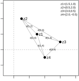
As an example, we report in Figure 1.3 a latent space representation, with

p= 2, of a network with n= 4 nodes. By graphical inspection, we may derive

thatz1 andz2 are exactly as close asz3 andz4; indeed,d(1,2) =d(3,4) = 1.41.

In Euclidean distance latent space model we may interpret this equal closeness

as an equal degree of similarity between the dyads (1,2) and (3,4). However,

such an interpretation would not be correct in the multiplicative model as

z₁0z2= 2.756=z30z4= 5.75. Latent coordinatesz3 and z4 are further from the

origin then z1 and z2, and thus the dyads (1,2) and (3,4) interact differently.

Hence, when the aim is at representing node similarities in the latent space, distance models seem to be providing with a more easily interpretable solution.

Also, the coordinates of nodes 3 and 4,z3 andz4, are equidistant from that of

nodes 1 and 2. Indeed, the Euclidean distances, d(1,3) =d(1,4) = 1.58 and

d(2,3) =d(2,4) = 2.92, capture it and give the idea that node 3 and 4 interact

in the same way with node 1 and node 2. This same interpretation does not hold with a multiplicative latent space model, as, for example, node 3 has an

higher probability to interact with node 1 than node 4, as z₁0z3 = 5.00 while

z₁0z4= 2.50.

A feature of the multiplicative model is that it guarantees, via the inner

(26)

either sign(z_i0zj) = sign(z0jzl) = sign(zl0zi) = 1, or sign(z0izj) = 1 and

sign(z_j0zl) = sign(z0lzi) = 0, where 1 denotes positive sign and 0 negative

sign. Such feature enforces a strong notion of transitivity in the latent space.

Indeed, given any node i, any two nodes (j, l) interacting with it have to

interact between themselves with a behaviour dictated by nodei. For example,

if nodei“relates” with both nodes j andl, then nodesj andlshould relate as

well. The allowed relationships are of the form “a friend of mine is a friend of mine” and “an enemy of a friend of mine is my enemy”. The configuration “an enemy of a friend of mine is a friend of mine” can not be represented. Instead, the distance model poses no explicit restriction on the relation between the distances between any three points, other than the usual triangular inequality,

d(i, j)≤d(i, l) +d(l, j). ● ● ● ● 0 1 2 3 4 −1 0 1 2 3 p=1 p=2 d(1,2) d(1,3) d(1,4) d(2,3) d(2,4) d(3,4) z1 z2 z3 z4 z1=(1.5,1.0) z2=(0.5,2.0) z3=(3.0,0.5) z4=(2.0,−0.5)

Figure 1.3. Two examples of a latent space representation of a network.

• Latent space models based onultrametrics. Schweinberger and Snijders,2003

consider a latent space build on an ultrametric. The ultrametric imposes stronger relations between the nodes than those imposed by the Euclidean

distance. In particular, given a function d(·) and two nodesi, j, we have that

d(i, j)≤max[d(i, l), d(l, j)]≤d(i, l) +d(l, j), for any other nodel. The first,

more restrictive, bound is encountered when the function is an ultrametric, the second when it is a metric (as it is the case with the Euclidean distance). In particular, the ultrametric condition implies that all the triangles are isosceles; there could not be all different values of the ultrametric function computed between any dyads, and this corresponds to at least two equal edge probabilities

(27)

1.3 Latent space models 11

Due to the complex structure of network data, latent space models for networks have been always estimated within a Bayesian framework by adopting a Gaussian representation for the latent coordinates. The two main approaches are standard MCMC algorithms, which usually provide faithful estimates but have potentially long computational times, and variational Bayes algorithm, whose estimation is quite fast but often suffers from numerical instability problems. The trade-off between feasible computational times and reliability of the estimates is crucial and should always be considered when choosing the inferential approach to be used for model estimation.

1.3.1 Latent space models for multidimensional networks

A couple of decades ago, analysing multidimensional network data corresponded to find a way to aggregate the views into a single one, and then analyse the “collapsed” network with standard models available for single networks. Some well known datasets in single networks literature, as for example the “Zachary karate club” dataset, are the result of such an “aggregation”. After these first attempts in multiplexes modelling, models specifically designed to deal with multiple views have been developed. In particular, in the context of latent space models, while the majority of the models have been designed specifically for single networks, several latent space models tailored to multidimensional networks have been proposed. Among such models, a distinction has to be made between latent space models for multidimensional network data and those for dynamic network data. Indeed, latent space models for dynamic networks assume temporal dependence between the networks and aim at capturing the potential evolution of the latent space trough time.

An example is the modelling framework developed by Sarkar and Moore,2005, later

extended by Sewell and Chen, 2015, where it is assumed that node-specific latent

coordinates evolve trough time, that is through the subsequent networks, following a first order Markov process. The dynamic component in the data is addressed, and the latent spaces serve to capture and visualize changes of the interactions between the nodes through time. The modelling framework proposed by Sewell

and Chen, 2015 is quite flexible and allows also to model, with small adjustments,

weighted network data or clustering tendencies in dynamic network data. Up to our knowledge, latent space models for dynamic networks with “longer memory” have not yet been proposed. For a more detailed descriptions of latent space models for

dynamic network data, we refer to Kim et al., 2018.

Differently from dynamic networks, views in multiplex data can not be modelled by using a predetermined structure; no consequentiality can be assumed between the networks, and neither any pre-specified association rule. Thus, different aims can be pursued when modelling multidimensional network data. We may summarize such aims into, at least, three different questions:

1. How do the nodes interact at a single view level?

2. Are the node-specific behaviours in the networks somehow associated? 3. Is there any common tendency in the node-specific behaviours across the views?

(28)

Depending on the data at hand and the modelling purposes, we may be interested in only one of the above questions, two of them or all three. Single views node interactions have usually been modelled via single-network latent spaces. Basic

models as the one proposed by Sweet, Thomas, and Junker,2013do not consider any

“higher level” structure beyond the single-network level, but other authors proposed different ways to address the global node behaviours. One example is that of the

model by Salter-Townshend and McCormick, 2017, which aims at capturing the

associations between single network latent spaces, corresponding to different views in the multiplex, by means of association parameters defined for each couple of networks. Such a model can be quite useful when the purpose is to synthetically capture which views are similar or dissimilar. However, when the number of views is high, this approach does not provide an easily interpretable insight on the overall structure underlying the observed multidimensional network. A different approach

has been proposed by Gollini and Murphy, 2016, who proposes to combine the

information coming from different networks assuming that these have been generated by a joint latent space. Such a framework permits to have a look both at

node-specific coordinates in the single networks and in the global (joint) representation.

For a more detailed description of the model by Gollini and Murphy,2016, we refer

to the corresponding paper and to AppendixD. Later, single-network latent spaces

are summarized by Durante, Dunson, and Vogelstein, 2017, which assumes that

the K different views have been generated by a mixture of H ≤K latent spaces.

Motivated by aK = 42 views brain multiplex, such framework may be useful when

the number of networks is quite high. Indeed, as networks are “units” belonging to

the H mixture components, few network-units correspond to a component, and this

could be a too small sample size for a mixture model. All of the above models have been derived in the context of binary multidimensional network data.

The following section will give an overview of the remaining chapters and appendixes.

1.4 Chapter summaries

Chapter 2presents an extension of the latent space model by Hoff, Raftery, and

Handcock, 2002 to model multidimensional network data. The proposed model

structure aims to capture shared similarities between the nodes in a single latent space, when different networks are assumed to be different realizations of a single underlying phenomenon. The model is used to describe the potential affinities between competing Countries in the Eurovision Song Contest during the period 1998-2015, with the aim to verify whether the observed votes exchange was influenced by such affinities.

The contents of Chapter 2 have been developed with Prof. Marco Alfò and Prof.

Thomas Brendan Murphy, and are reported in a paper which has been accepted for

publication in the Annals of Applied Statistics, see D’Angelo, Murphy, and Alfò,

2018. Also, the proposed model structure has been implemented in the R package

spaceNet, available on CRAN (https://CRAN.R-project.org/package=spaceNet).

Chapter3introduces a novel class of latent space models for multidimensional network

data analysis, which allows for node-specific effects. A parsimonious representation of the multiplex may be obtained, as a single latent space is employed to describe

(29)

1.4 Chapter summaries 13

the overall shared similarities between the nodes, while asymmetrical node features are captured by the node-specific effects. Various types of node-specific effects may be specified, in order to model different degrees of heterogeneity in nodes behaviours, both within and between networks.

The contents of Chapter3 have been developed with Prof. Marco Alfò and Prof.

Thomas Brendan Murphy, and are reported in a paper which is currently under first

revision in Social Networks, see D’Angelo, Alfò, and Murphy, 2018.

Chapter4 presents a latent space model for network and multidimensional network

data, which enables clustering of the nodes in the latent space. Clusters in the latent space correspond to communities of nodes in the multiplex, with clustering being a phenomenon which often arise in many observed network data, especially in social networks. Clustering structures are modelled using an infinite mixture distribution framework, which allows to perform joint inference on the number of clusters and the cluster parameters. The performance of the proposed method is illustrated through

an application to Vickers multiplex data (Vickers and Chan,1981), which represent

different social relations among a group of students.

Chapter4 is a pre-print and its content have been developed with Dr. Michael Fop

and Prof. Marco Alfò.

All the models developed in Chapters 2-4have been developed within a Bayesian

hierarchical framework, with inference on model parameters being carried out via MCMC algorithms.

AppendicesA-Creport the supplementary materials for Chapters2-4.

Last, Appendix D presents a different approach to estimate the lsjm model by

Gollini and Murphy, 2016, where inference is carried out via an MCMC algorithm,

instead of a Variational algorithm. In this Appendix, we prove that using a different procedure for model estimation we may obtain higher quality estimates. Also, we

propose a comparison with the model developed in Chapter 2. Such model may be

seen as a parsimonious version of the model by Gollini and Murphy,2016, where the

(30)

(31)

15

Chapter 2

Latent Space Models for

Multidimensional Networks

2.1 Introduction

The Eurovision Song Contest is a popular TV show, held since 1956, that takes place every year with participants from the countries member of the European Broadcasting Union. The competition has undergone several modifications through years and the number of participants has increased, together with the popularity of the show. Since its beginning, countries had to express their preferences for the competing songs through a voting system; representatives vote only for the songs that meet their tastes. Despite that, many issues of bias in the voting system have

been raised during the years (Yair, 1995). In the press and the literature, it has

often been claimed that votes are not only the expression of preferences for the songs, but for the performing countries themselves. Therefore, it has been claimed that the exchange of votes is not random but rather it is determined by some kind of similarity: the more two countries are close according to an unknown proximity measure, the more they will tend to vote for each other.

The exchange of votes in the Eurovision contest can be represented by means of a network, where the countries represent the nodes and the votes are recorded as edges. More specifically, within each annual edition of the Contest, the data may be

represented in the form of an adjacency matrixY, with generic elementyij = 1 if a

representative of countryivotes for a song by a performer from thejthcountry and 0

otherwise, where i, j= 1, . . . , n indexes countries. Network data can be represented

by means of graph theory. More formally, a network is thought to be the realization

of a graph G(N, E), whereN denotes the set of nodes andE the set of edges. The

number of observed nodes and edges will be denoted, respectively, by|N|=n and

|E|=e. Generally, the law generating the observed networks is unknown and several

different models have been proposed to describe such complex structures. Erdős and

Rényi, 1959 and Erdős and Rényi, 1960 modelled arch formation in a network as

arising from a random process: each dyad (i, j) is independent and the probability

of forming a link is constant over the network. This first model was generalized, both relaxing the assumption of constant edge probability over the network and the

(32)

p1 and p2 kept the assumption of independence among the dyads but increased

the number of parameters describing edge probabilities, to take into account the attractiveness of a node (the highest the value the highest the probability for this node to be connected with others) and the mutuality (the propensity of forming symmetric relations). The independence assumption on the dyads was then relaxed

via the introduction of Markov graphs by Frank and Strauss,1986, attempting to

model triangular relations in a network. Later onp∗ models or ERGMs (Exponential

Random Graph models) have extended the work done by Frank and Strauss,1986

introducing differnet summary statistics, see for example Krivitsky et al., 2009and

Robins et al.,2007. A different approach is the so-calledstochastic block model, which

attempts to decompose the nodes in different sub-groups, see Holland, Laskey, and

Leinhardt,1983, Airoldi et al.,2008. In its basic formulation, nodes within a group

have the same probability of forming edges, while this probability changes among

groups. Hoff, Raftery, and Handcock,2002 added an extra layer of dependence: the

observed edge formation process is assumed to be a function of nodes’ coordinates in a (low-dimensional) latent space. Two different specifications are considered, the

distance model, where the latent space is euclidean, and theprojection model, where

it is bilinear. The model by Hoff, Raftery, and Handcock, 2002has been extended

to perform clustering on the latent nodes’ coordinates by Handcock, Raftery, and

Tantrum, 2007. A generalization of the projection model by Hoff, Raftery, and

Handcock,2002is the multiplicative latent space model by Hoff, 2005, designed to

capture certain types of third-order dependence patterns in the network. Another approach that makes use of latent variables has been proposed by Snijders and

Nowicki,1997. This model is based on the stochastic block model by Holland, Laskey,

and Leinhardt,1983, where latent variables are introduced in the determination of

the nodes’ group memberships. A more exhaustive review of models for statistical

network analysis can be found in Goldenberg et al.,2010, Salter-Townshend et al.,

2012 and Murphy,2015.

The models presented above refer to single networks, that is, in the present context, to the modelling of one single edition of the Eurovision Song Contest or a summary of several editions. If a group of editions of the Contest is considered, many replications of the adjacency matrices, representing the preferences expressed by countries towards others, are available. Therefore, the data can be described by

a multidimensional network (or multiplex), Y = (Y(1), . . . ,Y(K)), which may be

thought of as the realization of a collection of graphsG= (G(1), . . . , G(K)), where

k = 1, . . . , K indexes editions. The generic graph G(k) = (N, E(k)) has the same

set of nodes N as the others (K−1) graphs in the collection (the participants to

the group of editions), but potentially different set of edges E(k) (the preferences

expressed in each edition). Hence, a multidimensional network describes different (independent) realizations of a relation among the same group of nodes. Different models have been developed to deal with this kind of data. Fienberg, Meyer, and

Wasserman,1985adapted a log linear model to the context of multiplex data. Greene

and Cunningham,2013 proposed to summarize the information coming from all the

different networks (views) aggregating them into a single one. Sweet, Thomas, and

Junker,2013proposed a Hierarchical Latent Space model, which generalizes network

latent space models to a collection of networks. The joint multiplex distribution factorizes into single network distributions, which are modelled independently and

(33)

2.2 The Eurovision Song Contest 17

inference is carried out via MCMC. Gollini and Murphy,2016 extended the latent

space model in Hoff, Raftery, and Handcock, 2002 to multiplex data, assuming

that the edge probabilities are function of a single latent variable. To estimate the joint latent space coordinates, they propose to use a variational Bayes algorithm and decompose the posterior distribution, fitting a different latent space to each network. Then, the separate estimates are employed to recover the joint latent space.

The multiplicative latent space model was extended by Hoff, 2015 to the context of

multidimensional networks. In that case, each network in the multiplex is modelled with its own latent space, independently from the others. Salter-Townshend and

McCormick,2017proposed a method to jointly model the structure within a network

and the correlation among networks via a Multivariate Bernoulli model. Another approach developed to describe the (marginal) correlation among different networks

in a multiplex has been proposed by Butts and Carley,2005. Hoff, 2011proposed

to model multiplex data as multiway arrays and applied low-rank factorization to

infer the underlying structure. Durante, Dunson, and Vogelstein, 2017 proposed a

Bayesian non-parametric approach to latent space modelling, where clustering is performed on the latent space dimensions in order to discriminate the most relevant ones for each view.

The present work aims at recovering the similarities among countries, modelling the exchange of votes during several editions of the Eurovision Song Contest. We

adopt a framework similar to that of Gollini and Murphy, 2016 and we consider

the projection of the countries into a common latent space. Similarities among countries are then expressed in terms of distances in this latent space. We introduce network-specific coefficient parameters to weight the relevance of the latent space in the determination of edge probabilities in each network. We consider the editions that took place after the introduction of the televoting system and focus on the period 1998-2015. Further, we consider geographical and cultural covariates in the analysis.

The paper is organised as follows. Section 2.2 summarizes the history of the

Eurovision Song Contest together with the principal works on the subject (section

2.2.1) and presents the analysed data (section2.2.2). Latent space models for network

data are introduced in section2.3and the proposed model is outlined in section2.3.1.

Model estimation is discussed in section 2.4. Further issues are discussed in section

2.5, such as model identifiability (section 2.5.1), missing data (section2.5.2) and the

introduction of edge-specific covariates (section 2.5.3). The application is presented

in section2.6 and the results are discussed in section2.7. A large scale simulation

study is outlined in section2.8, where also the main findings are reported. Section

2.9presents the results of a comparison between the proposed model and the lsjm

by (Gollini and Murphy, 2016). We conclude with some discussion in section2.10.

2.2 The Eurovision Song Contest

2.2.1 History of the contest and previous works on the subject

The Eurovision Song Contest, held since 1956, is a TV singing competition where the participant countries are members of the EBU (European Broadcasting Union). Despite its name, the European Broadcasting Union includes both European and

(34)

non European countries. Indeed, Eurovision’s fame has spread all over the world during the last years and it has been broadcast from South America to Australia. It is the non-sportive TV program with the largest audience in the world and one of

the oldest ones (Lynch,2015).

From its first edition, where only seven countries competed, there have been several changes in the number of participants, the voting system and the structure of the competition. Due to the increasing popularity of the program, many countries have been included in the contest. The current structure of the contest consists of two preliminary stages used to select the finalists, followed by the final stage for the title. The voting system has been modified several times, in the voting procedure and the grading scheme. In the early years of the competition, a jury elected the winning

song. Later, the system has been supported by televoting 1_{, introduced in 1998 in}

all the competing countries. As for the grading scheme, it is positional2 _{since 1962,}

but the method used to rank the countries has been modified across the different editions. From 1975 to 2015, each country had to express its top ten preferences ranking them from the most to the least favourite using the following scores: 12, 10, 8, 7, 6, 5, 4, 3, 2, 1. Each country had to vote exactly ten others, could not vote for itself and each grade could be used only once. At the end, the country receiving the highest overall score would have won the competition. A restriction has been imposed on the lyrics in the past, as the participants were required to perform a song written in their national language. However, this rule was definitively abolished after 1998.

Every year, both the singer and the song representing a country change, making each edition of the Eurovision independent from the previous one. Indeed, the structure of the competition is built in such a way that the past results will not influence the future performances. Countries should vote only according to their tastes and, as musical evaluation has no objective criteria, the voting results should not depend on the countries themselves, but only on the songs. However, this claim was often doubted, especially after the introduction of televoting. Several issues have been raised on the voting system, which was said to be biased. The first paper

investigating the presence of bias in the voting system is Yair, 1995. This work

considers voting relations among 22 of the 24 countries competing in the period 1975-1992 and claims that, according to their voting preferences, they can be clustered in three regional blocks: Mediterranean, Western and Northern. Countries tend to vote

for others from the same block, hence following a non-objective (non-democratic)

behaviour. However, the paper does not provide an in-depth statistical evaluation of the results. The author supports the theory that the geographic location of a country may influence its voting behaviour. This assumption has been further

investigated by Fenn et al., 2006; in this work, the dynamic evolution of votes

exchanged in the competition 1992 to 2003 has been analysed, with the aim at looking for sub-groups of countries. The sub-groups found are not fully explained by

1

Televoting is a voting method conducted by telephone. The organizers of the event provide the audience with telephone numbers associated with the different participants. The rankings are then determined by the number of calls/SMS that each contestant receives.

2_{Positional voting is a ranked voting system where a list of candidates has to be ordered by}

voters. Rankings of different voters are converted into points and cumulated in scores, associated with each contestant. The one receiving the highest final score wins.