Grade Eximia cum laude approbatur Instructor Jukka Corander
PCSI-labeled Directed Acyclic Graphs
Jarno Lintusaari
Helsinki April 8, 2014
UNIVERSITY OF HELSINKI
Faculty of Science Department of Mathematics and Statistics Jarno Lintusaari
PCSI-labeled Directed Acyclic Graphs
Applied Mathematics
April 8, 2014 44 pages + 1 appendices
Directed Acyclic Graph, Bayesian networks, Context-specific independencies, Bayesian model learning This thesis proposes a generalization for the model class of labeled directed acyclic graphs (LDAGs) introduced in Pensar et al. (2013), which themselves are a generalization of ordinary Bayesian works. LDAGs allow encoding of a more refined dependency structure compared to Bayesian net-works with a single DAG augmented with labels. The labels correspond to context-specific indepen-dencies (CSIs) which must be present in every parameterization of an LDAG. The generalization of LDAGs developed in this thesis allows placement of partial context-specific independencies (PCSIs) into labels of an LDAG model, further increasing the space of encodable dependency structures. PCSIs themselves allow a set of random variables to be independent of another when restricted to a subset of their outcome space. The generalized model class is named PCSI-labeled directed acyclic graph (PLDAG).
Several properties of PLDAGs are studied, including PCSI-equivalence of two distinct models, which corresponds to Markov-equivalence of ordinary DAGs. The efficient structure learning algorithm introduced for LDAGs is extended to learn PLDAG models. This algorithm uses a non-reversible Markov chain Monte Carlo (MCMC) method for ordinary DAG structure learning combined with a greedy hill climbing approach. The performance of PLDAG learning is compared against LDAG and traditional DAG learning using three different measures: Kullback-Leibler divergence, number of free parameters in the model and the correctness of the learned DAG structure. The results show that PLDAGs further decreased the number of free parameters needed in the learned model compared to LDAGs yet maintaining the same level of performance with respect to Kullback-Leibler divergence. Also PLDAG and LDAG structure learning algorithms were able to learn the correct DAG structure with less data in traditional DAG structure learning task compared to the base MCMC algorithm.
Tekijä — Författare — Author Työn nimi — Arbetets titel — Title Oppiaine — Läroämne — Subject
Työn laji — Arbetets art — Level Aika — Datum — Month and year Sivumäärä — Sidoantal — Number of pages Tiivistelmä — Referat — Abstract
Avainsanat — Nyckelord — Keywords
Säilytyspaikka — Förvaringsställe — Where deposited Muita tietoja — övriga uppgifter — Additional information
Contents
1 Introduction 1
2 Theory of PLDAGs 5
3 Bayesian learning of PLDAGs 25
4 Experimental setting and results 33
5 Discussion 40
Appendices
1
Introduction
The aim of this thesis is to generalize the theory of Labeled Directed Acyclic Graphs (LDAGs) introduced in Pensar et al. (2013), to implement an algorithm for learning these generalized labeled DAGs from data, and to evaluate its performance against traditional Bayesian networks and LDAGs.
This thesis has been written so that the reader is not required to refer back to Pensar et al. (2013) in order to fully follow the development of the generalization. Nevertheless the reader should be familiar with the theory of Bayesian networks, basic probability calculus and Bayesian inference. The text explains the concepts introduced for LDAGs, provides their generalizations and introduces new concepts required by the generalization. The key differences between LDAGs and their gen-eralization are also discussed when needed.
1.1
LDAGs and context-specific independencies
As with Bayesian networks the basic idea of LDAGs is to provide a graphical rep-resentation of the dependency structure of a joint distribution over a set of random variables. LDAGs are a generalization of Bayesian networks, providing a way to express more refined dependency structures by allowing a node to be independent of some of its parents in certain contexts. In LDAGs, these context-specific inde-pendencies are denoted with labels attached to the edges of the DAG. One of the concrete benefits of including context-specific independencies to graphical models is the possibility for a substantial reduction in the parameteric dimensionality of the model (Boutilier et al., 1996; Friedman and Goldszmidt, 1996; Poole and Zhang, 2003; Koller and Friedman, 2009; Pensar et al., 2013).
The idea of context-specific independecies (CSIs) in graphical models is not new, and has been studied in the literature (Boutilier et al., 1996; Friedman and Goldszmidt, 1996; Chickering et al., 1997; Eriksen, 1999; Poole and Zhang, 2003; Koller and Friedman, 2009). The main benefit of LDAGs over these previous works is the compact way of representing a dependency structure with CSIs through a single DAG augmented with labels. The cost is a slightly reduced space of encodable CSIs. The use of labels was originally introduced in Corander (2003) for considering CSIs in undirected graphical models.
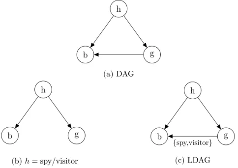
and Heckerman (1996), p. 52 is given:
A guard of a secured building expects three types of persons (h) to approach the building’s entrance: workers in the building, approved visitors, and spies. As a person approaches the building, the guard can note its gender (g) and whether or not the person wears a badge (b). Spies are mostly men. Spies always wear badges in an attempt to fool the guard. Visitors don’t wear badges because they don’t have one. Female workers tend to wear badges more often than do male workers. The task of the guard is to identify the type of person approaching the building.
This scenario can be represented by the DAG on top in Figure 1a. The ordinary DAG cannot represent the fact that given a person is a spy or a visitor the badge wearing is independent of the gender of the person. This would require a DAG shown in subgraph 1b which again would not be the correct DAG if the person was a worker. The LDAG in subfigure 1c combines these two graphs by adding a label marking the edge as removable when the person is either a spy or a visitor. All the parameterizations of the LDAG in subfigure 1c are required to encode this local CSI to the conditional probability distribution of b given its parents. Addition of this CSI decreases the number of free parameters in the model.
h b g (a) DAG h b g (b)h= spy/visitor h b g {spy,visitor} (c) LDAG
1.2
Introducing partial CSIs for LDAGs
Consider the spy/visitor/worker -example given above. It was stated that spies are mostly men but the gender distribution of visitors and workers was left open. Making an additional assumption that the gender distribution of workers in the buildings is the same as with the approved visitors allows us to combine the parameters of the conditional distribution of gender (g) for these two parental outcomes. This again leads to a reduction in the number of free parameters in the model. This kind of an independence is named partial CSI (PCSI) because it does not include all of the outcomes of the parent in consideration. In this case the gender distribution of spies is different from the gender distribution of workers and visitors. An LDAG including PCSIs is named PLDAG and is the generalization developed in this work. An example of a PLDAG model corresponding to the situation described above is given in Figure 2. Note that the PCSI has no specific context in this case and is always in effect. The superscript in the label denotes the outcomes of the parent which will result in a similar distribution of gender. In the case of the CSIs this superscript is not needed as they result in the same distribution with all outcomes of the corresponding parent.
h
b g
{}worker,visitor
{spy,visitor}
Figure 2: A PLDAG describing the spy/visitor/worker -scenario
A sibling for PCSI is a contextual weak independence (CWI) proposed by Wong and Butz (1999) for Bayesian networks. This approach relies in the use of multiple Bayesian networks called Bayesian multinets introduced by Geiger and Heckerman (1996). As with LDAGs, the difference between PLDAGs and this approach is the ability of PLDAGs to compactly represent the whole dependency structure with a single DAG augmented with labels. The cost is a slightly reduced space of encodable PCSIs. When comparing the definitions of PCSI and CWI, the latter is more general in allowing one to restrict also the child variable outcome space in order to expose the independency. It would be possible to introduce also CWIs for LDAGs but they would require a more complex labeling system.
As will be shown in this work, PLDAGs maintain the advantageous properties of LDAGs bringing the ability to further refine the dependency structure and decrease the parametric dimension of the model. In the end of the Theory section both PCSI-separation between sets of variables and PCSI-equivalence of two different PLDAGs are investigated. Then the algorithm for LDAG structure learning introduced in Pensar et al. (2013) is extended to learn PLDAG structures. Finally the experiment section will show how these algorithms compare and bring improvement even in the standard DAG structure learning.
2
Theory of PLDAGs
The following notations are used throughout the text. A DAG will be denoted by
G = (V, E) where V = (1, . . . , d) is the set of nodes and E ⊂ V ×X is the set of edges such that if (i, j) ∈ E then the graph contains a directed edge from node i
to j. Let j be a node in V. If (i, j)∈ E then the node i is called a parent of node
j. The set of all parents of j is denoted with Πj. The nodes in V provide indexes
for a corresponding stochastic variables X1, . . . Xd. Due to the close relationship
between a node and its corresponding variable, the terms node and variable are used interchangeably. Small letters xj are used to denote a value taken by the
corresponding variable Xj. If S ⊆ V, then XS denotes the corresponding set of
variables andxS a value taken by XS. The outcome space of variableXj is denoted
by Xj and the joint outcome space of a set of variables by the Cartesian product XS =×j∈SXj. The cardinality of the outcome space of XS is denoted by|XS|.
An ordinary DAG encodes independence statements in the form of conditional in-dependencies.
Definition 1. Conditional Independence (CI)
Let X ={X1, . . . Xd} be a set of stochastic variables where V ={1, . . . , d} and let
A, B, S be three disjoint subsets of V. XA is conditionally independent ofXB given
XS if the equation
p(XA=xA |XB =xB, XS =xS) =p(XA=xA|XS =xS)
holds for all (xA, xB, xS)∈ XA× XB× XS wheneverp(XB =xB, XS =xS)>0. This
will be denoted by
XA ⊥XB |XS.
If we let S = ∅, then conditional independence simply corresponds to ordinary independence between variables XA and XB.
A fundamental property of Bayesian networks is the directed local Markov property stating that variable Xj is conditionally independent of its non-descendants given
its parental variablesXΠj. This property gives rise to the factorization along a DAG
p(X1, . . . , Xd) = d
Y
j=1
p(Xj |XΠj), (1)
for any such joint distribution of variables X1, . . . Xj, that conform to the
joint distribution is defined by the set of conditional probability distributions (CPDs) over the variablesXj conditioned to their respective parents in the DAG. A Bayesian
network is then defined by parameterizing these CPDs. In discrete cases a frequently used tool is a conditional probability table (CPT) which will be used here as well. As there is a direct correspondence, the terms CPT and CPD are used interchangeably. The local structures in the DAG, i.e. a child node with its parents, can be seen as modules of the DAG composing the whole. The joint distribution is defined through these modules or local structures by the factorization (1). It is therefore natural to implement any refinement of the dependency structure through these local structures. It is not only a good convention but the LDAG structure learning section will also show clear benefits from computational performance point of view. In practice this means that the various types of context-specific independencies are set into the local structures by setting restrictions for their corresponding CPDs. Next the different types of context-specific independencies are defined in their gen-eral form. Then the way to place them into the local structures of a DAG through lables is defined. The following notion of context-specific independence was formal-ized by Boutilier et al. (1996).
Definition 2. Context-specific Independence (CSI)
Let X ={X1, . . . Xd} be a set of stochastic variables where V ={1, . . . , d} and let
A, B, C, Sbe four disjoint subsets ofV. XAis contextually independent ofXB given
XS and the context XC =xC if the equation
p(XA =xA|XB =xB, XC =xC, XS =xS) =p(XA=xA|XC =xC, XS =xS)
holds for all (xA, xB, xS) ∈ XA× XB × XS whenever p(XB = xB, XC = xC, XS =
xS)>0. This will be denoted by
XA⊥XB |XC =xC, XS.
Before introducing the notion of partial CSI we need definitions of partial indepen-dence and partial conditional indepenindepen-dence.
Definition 3. Partial Independence
LetX, Y be discrete stochastic variables, X andY their respective outcome spaces,
y∈ Y for which p(y)>0 and denote ¯
y={y0 ∈ Y :p(X =x|Y =y0) =p(X =x|Y =y) (2)
We say that X is partially independent of Y in y∗ if |y∗| > 1 where y∗ ⊆ y¯. This will then be denoted by
X ⊥Y |Y ∈y∗.
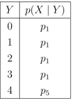
Consider the conditional probability table (CPT) given in Figure 3. Here X is partially independent ofY by ¯1, where ¯1 = {0,1,2,3}. Note that ¯0 = ¯1 = ¯2 = ¯3 and we could have replaced ¯1 with any of them. We can see that if also p5 = p1, then
¯
1 =Y and partial independence by Y yields the standard independence between X
and Y. Y p(X |Y) 0 p1 1 p1 2 p1 3 p1 4 p5
Figure 3: CPT defining a partial independence
Y Z p(X |Y, Z) 0 0 p1 1 0 p1 2 0 p3 0 1 p4 1 1 p4 2 1 p6
(a) Partial Conditional Independence
Y Z p(X |Y, Z) 0 0 p1 1 0 p1 2 0 p3 0 1 p4 1 1 p5 2 1 p6 (b) PCSI Figure 4: CPT:s representing different type of independencies Definition 4. Partial Conditional Independence
Let X ={X1, . . . Xd} be a set of stochastic variables where V ={1, . . . , d} and let
xS)>0 for all xS ∈ XS and denote
¯
xB ={x∗B ∈ XB : p(XA=xA|XB=x∗B, XS =xS) =
p(XA=xA|XB=xB, XS =xS),
p(XB =x∗B, XS =xS)>0 for all (xA, xS)∈ XA× XS}.
We say thatXAis partially conditional independent ofXBinXB∗ givenXSif|XB∗|>1
where X∗
B ⊆x¯B. This will then be denoted by
XA⊥XB |XB ∈ XB∗, XS.
In Figure 4a is given an example of a partial conditional independence of the type
X ⊥ Y | Y ∈ {0,1}, Z. We can see that this does not hold in the CPT in Figure 4b, unless we specifically set Z = 0. This observation leads us to the definition of Partial Context Specific Independence generalizing the definition of Context-Specific Independence (CSI) in Pensar et al. (2013) and Boutilier et al. (1996).
Definition 5. Partial Context-Specific Independence (PCSI)
Let X = {X1, . . . Xd} be a set of stochastic variables where V = {1, . . . , d} and
let A, B, C, S be four disjoint subsets of V. Let xB ∈ XB and xC ∈ XC for which
p(XB =xB, XC =xC, XS =xS)>0 for allxS ∈ XS and denote {x¯B}xC ={x ∗ B ∈ XB : p(XA=xA|XB =x∗B, XC =xC, XS =xS) = p(XA=xA|XB =xB, XC =xC, XS =xS), p(XB =x∗B, XC =xC, XS =xS)>0 for all (xA, xS)∈ XA× XS}.
We say that XA is partially contextual independent of XB in XB∗, given XS and
XC =xC if |XB∗|>1 whereX
∗
B ⊆ {x¯B}xC. This will then be denoted by
XA⊥XB |XB ∈ XB∗, XC =xC, XS.
We say that two PCSIs aresimilar if they differ only in the context XC =xC.
When {x¯B}xC = XB, a direct calculation shows that a PCSI XA ⊥ XB | XB ∈ XB, XC = xC, XS is equivalent with a CSI XA ⊥ XB | XC = xC, XS. Similarly
partial conditional independence is equivalent to conditional independence and par-tial independence to independence when {x¯B}xC = XB and y = Y respectively.
Note however that if the independence is genuinely partial (i.e. {x¯B}xC 6=XB) then
partial independencies lack two common properties of independencies highlighted in the next remark.
Remark 1. LetXC =xC be a context and let{x¯B}xC 6=XB. Then
XA⊥XB |XB ∈ {x¯B}xC, XC =xC, XS
6⇒ (3)
p(XA =xA|XB =xB, XC =xC, XS =xS) =p(XA=xA|XC =xC, XS =xS)
for any xB ∈ {x¯B}xC and (xA, xS)∈ XA× XS. Also
XA⊥XB |XB ∈ {x¯B}xC, XC =xC, XS
6⇒ (4)
XB ⊥XA|XA∈ XA, XC =xC, XS.
The objective is to introduce PCSIs to directed acyclic graphs. As DAGs provide the factorization (1) of the joint probability distribution according to the graph families we will use parent configurations as contexts for the PCSIs in the similar manner as for CSIs in Pensar et al. (2013). The word local is used to refer to a graph family. Definition 6. Local PCSI in a DAG
A PCSI in a DAG is local if it is of the form Xj ⊥XB |XB ∈ XB∗, XC =xC, where
Πj =B∪C, i.e. B and C form a partition of the parents of nodej. A local PCSI
is called modular, if it can be induced from a set of simple local PCSIs of the form
Xj ⊥Xi |Xi ∈ Xi∗, XC =xC, wherei∈Πj and C = Πj\ {i}.
Only simple local PCSIs will be used in PLDAGs. They allow keeping the labeling system concise and easy to interpret. The unevitable cost of this choice is that non modular PCSIs are not representable by PLDAGs. In practice this means that arbitrary rows in a CPT cannot be combined with a single label, but combined rows must share the same parent configuration (context) for all but one parent. By combining labels more complicated PCSIs can be built when needed. This corresponds to a procedure of building context-specific independencies by dropping out parents one by one. One benefit brought by introducing PCSIs for LDAGs is that it expands the number of local CSIs that can be represented. From now on the phrase local PCSI is used to refer to a modular local PCSI since all local PCSIs encoded by a PLDAG will be modular by definition.
Definition 7. PCSI Labeled Directed Acyclic Graph (PLDAG)
LetG= (V, E) be a DAG over stochastic variables {X1, . . . , Xd}. For all (i, j)∈E
as the set
LDi
(i,j)={xL(i,j) ∈ XL(i,j) :Xj ⊥Xi |Xi ∈ Di, XL(i,j) =xL(i,j)}.
where Di ⊆ Xi and |Di| >1. We call Di the domain of the label LD(i,ji). A PLDAG
denoted by GP L = (V, E,LDE) is a DAG appended with a label set L
D
E of unempty
PCSI-labels LDi
(i,j).
A PLDAG is a DAG augmented with additional local independency conditions that a distribution over the stochastic variables {X1, . . . , Xd} is required to fulfill. All
elements xL(i,j) of a label L
Di
(i,j) provide contexts for similar simple local PCSIs.
Note that an edge (i, j) may have more than one label attached to it. If for some PCSI-label LDi
(i,j) it holds that Di = Xi then this label corresponds to an LDAG
label L(i,j) defined in Pensar et al. (2013). Such a label represents a local CSI and
therefore is called also a CSI-label. In Figure 5 there is an example of a PLDAG and a corresponding CPT that follows the dependency structure represented by the PLDAG. The superscripts of the labels represent the set Di in the notation and
are left without the curly brackets for the purpose of making the appearance of the notation clearer. Figure 6 shows the corresponding local PCSI statements.
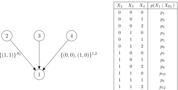
2 3 4 1 {(1,1)}X2 {(0,0),(1,0)}1,2 X2 X3 X4 p(X1|XΠ1) 0 0 0 p1 0 0 1 p2 0 0 2 p2 0 1 0 p4 0 1 1 p5 0 1 2 p6 1 0 0 p7 1 0 1 p8 1 0 2 p8 1 1 0 p10 1 1 1 p5 1 1 2 p12
LX2 (2,1) ={(1,1)} ⇒X1 ⊥X2 |X2 ∈ X2, (X3, X4) = (1,1) ⇒X1 ⊥X2 |(X3, X4) = (1,1) L{(41,,1)2} ={(0,0),(1,0)} ⇒X1 ⊥X4 |X4 ∈ {1,2}, (X2, X3) = (0,0)∨(X2, X3) = (1,0)
Figure 6: Local PCSIs from the labels of the PLDAG in Figure 5.
2.1
Properties of PLDAGs
In many cases DAGs provide a representation of the dependency structure between variables that is easy to interpret. Labeled DAGs provide a way to represent more refined dependency structures yet maintaining the interpretability of the represen-tation. In order to facilitate this property of labeled DAGs two conditions originally introduced for LGMs in Corander (2003) were applied to LDAGs in Pensar et al. (2013), namely maximality and regularity. By definition it is possible to represent the same local CSIs with different labelings. For example a certain set of local CSIs can induce other local CSIs that may not be explicitly defined in the corresponding labelings. Maximality ensures that every LDAG label includes all applicable local CSIs. It is also possible to define a set of local CSIs forming a CI and rendering a variable completely independent of its parent. This is equivalent to removing the corresponding edge from the underlying DAG. Regularity ensures that the local CSIs in the labels are minimal in the sense that no subset of them can be represented by removing an edge from the underlying DAG. These two conditions together define an unique and clear representation for LDAGs. They will be next generalized for PLDAGs with the aid of a condition called conciseness.
Definition 8. Concise PLDAG
Let GP L = (V, E,LDE) be a PLDAG. We say that GP L is concise if for any two
distinctLDi
(i,j),L
Ai
(i,j) ∈ L
D
E where (i, j)∈E it holds that
1. Di 6=Ai
2. If Di∩ Ai 6=∅ then L(Di,ji)∩ LA(i,ji)=∅.
Proof. LetGP L = (V, E,LDE) be a PLDAG, (i, j)∈E,L Di (i,j) ∈ L D E andxL(i,j) ∈ L Di (i,j).
The element xL(i,j) and its corresponding label L
Di
(i,j) represent a local PCSI Xj ⊥
Xi | Xi ∈ Di, XL(i,j) = xL(i,j). Therefore we can always combine the elements of two distinct labelsLDi
(i,j),L
Ai
(i,j) ∈ L
D
E whereDi =Ai without altering the dependency
structure represented by the labels. This ensures existence of a form where condition 1 in Definition 8 is satisfied. Next we define two properties of labels. We use the word represent to refer to both explicitly represented PCSIs in the labels and to those derived from them.
Property 1. If for some xL(i,j) ∈ XL(i,j), Xj ⊥ Xi | Xi ∈ Di, XL(i,j) = xL(i,j) and
Xj ⊥ Xi | Xi ∈ Di0, XL(i,j) = xL(i,j) where Di ∩ Di
0
6
= ∅ are two local PCSIs represented by the PLDAG, then Xj ⊥ Xi | Xi ∈ Di ∪ Di0, XL(i,j) = xL(i,j) is represented by the PLDAG. This follows directly from Definition 5.
Property 2: If Xj ⊥ Xi | Xi ∈ Di, XL(i,j) = xL(i,j) is represented by the PLDAG then also Xj ⊥Xi |Xi ∈ Di0, XL(i,j) =xL(i,j) is represented by the PLDAG for any
Di0 ⊆ Di. This follows also directly from Definition 5.
Next we relabelGP L to another form and show that it is concise. Since condition 2
in Definition 8 is edge specific, we can concentrate on one edge (i, j) at a time. Let
LD
(i,j)⊆ L
D
E be the labels on the edge (i, j) in GP L. LetD(xL(i,j)) be the setDi ⊆ Xi for which the corresponding PCSIs are represented in GP L. We assumeD(xL(i,j)) is maximal in the sense that it includes all PCSIs that are represented for the edge in question. LetG∗P L = (V, E,LD∗
E ) be a PLDAG where eachxL(i,j) in the labels ofL
D
E
is contained only in the labelLDi∗
(i,j) whereDi
∗ ∈ Di
(xL(i,j)). It follows from Property 1 above that all sets inD(xL(i,j)) are disjoint which in turn with the construction of
LD∗
E satisfies condition 2 for G
∗
P L. From Property 2 above and the construction of D(xL(i,j)) it follows that all local PCSIs represented by labels inGP L are represented by labels in G∗P L and that they are the only ones.
Definition 8 causes the representation of PLDAG to be concise, preventing overlap-ping PCSI definitions in the labels. From the proof of Proposition 1 one can derive a method for relabeling a PLDAG to a concise form. First one combines labels for which Di =Ai on the same edge. Then repeating until there are no more changes
one adds thosexL(i,j) ∈ L
Di
(i,j)∩ L
Ai
(i,j) that do not fulfill condition 2 (Def. 8) to a label
LDi∗
(i,j) where Di∗ = Di ∪ Ai and removes them from both L
Di
(i,j) and L
Ai
(i,j). Figure
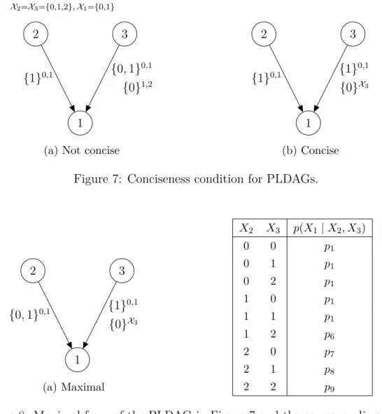
7a represents a PLDAG that is not concise. The labels on the edge (3,1) are over-lapping on the element 0. By applying the method given above we get the concise PLDAG in Figure 7b. As all PLDAGs can be relabeled to fulfill Definition 8 it is
used as a basis for the definitions of maximality and regularity for PLDAGs. X2=X3={0,1,2},X1={0,1} 2 3 1 {1}0,1 {0,1} 0,1 {0}1,2
(a) Not concise
2 3 1 {1}0,1 {1} 0,1 {0}X3 (b) Concise Figure 7: Conciseness condition for PLDAGs.
2 3 1 {0,1}0,1 {1} 0,1 {0}X3 (a) Maximal X2 X3 p(X1 |X2, X3) 0 0 p1 0 1 p1 0 2 p1 1 0 p1 1 1 p1 1 2 p6 2 0 p7 2 1 p8 2 2 p9
Figure 8: Maximal form of the PLDAG in Figure 7 and the corresponding CPT. Definition 9. Maximal PLDAG
Let GP L = (V, E,LDE) be a concise PLDAG. We say that GP L is maximal if the
following conditions hold:
1. The domain set Di of an element xL(i,j) ∈ L
Di
(i,j) can not be extended without
inducing an additional local PCSI to GP L.
2. No elementxL(i,j) ∈ XL(i,j) can be added to a labelL
Di
(i,j)without either inducing
an additional local PCSI or breaking conciseness. Note that adding an element to an empty label LDi
(i,j) is understood as including the
label into LD
The conditions in Definition 9 preserve the dependency structure of the original PLDAG. Note that in case of LDAGs the definition of conciseness is not needed because of the simpler model structure. To provide an illustration of maximality, in Figure 8a there is an element added to a label of the PLDAG in Figure 7b. Any further addition or extension of the labels would either yield an additional local PCSI or render the PLDAG not concise. Therefore the PLDAG is maximal.
The next theorem generalizes Theorem 1 in Pensar et al. (2013) for PLDAGs. Theorem 2. LetGP L = (V, E,LDE)andG
0
P L = (V, E,L
0A
E)be two maximal PLDAGs
with the same underlying DAG GL= (V, E). Then GP L and G0P L represent
equiva-lent dependency structure if and only if LD
E =L0AE, i.e. GP L =G0P L.
Proof. LetGP L = (V, E,LDE) andG0P L = (V, E,L0AE) be maximal PLDAGs with the
same underlying DAGGL= (V, E). Since they have the same underlying DAG, only
the labelings can render the dependency structures different. If they have the same labelings they must then represent the same dependency structures. Assume then that they represent the same dependency structure but have different labelings, i.e.
LD
E 6=L
0A
E. It means that there exists at least one label with an element that is not
found in both of the labelings. We can therefore assume that L0A
E has an element
x0(i,j) ∈ L0Ai
(i,j) that is not in the corresponding labelL
Ai
(i,j) ∈ L
D
E in the other PLDAG.
This element-label pair corresponds to a local PCSI Xj ⊥ Xi | Xi ∈ Ai, XL(i,j) =
x0L
(i,j). Because the PLDAGs represent the same dependency structure, the local PCSI has to nevertheless hold forGP L as well. This implies that x0L(i,j) can be added toLAi
(i,j) without inducing an additional local PCSI. IfGP L remains concise after the
addition, it was not maximal and we have a contradiction. If addition renderedGP L
non-concise there must exist a setA∗
i ⊆ XL(i,j) for whichx
0
(i,j)∈ L
A∗
i
(i,j)andDi ⊂ A(i,j)
by maximality of GP L. This means that a local PCSI Xj ⊥ Xi | Xi ∈ A∗i, x
0
L(i,j) holds forGP L and therefore forG0P L as well. But nowG
0
P L cannot be maximal since
for the element x0L
(i,j) ∈ L
0Ai
(i,j) the set Ai can be extended to A∗i without inducing
an additional local PCSI.
Definition 10. Underlying LDAG
Let GP L = (V, E,LDE) be a PLDAG. An underlying LDAG of GP L is the LDAG
GL = (V, E,LE), where LE is acquired from LDE by removing all the labels L
Di
(i,j)
fromLD
E for which Di 6=Xi, i.e. the domain is not maximal.
Proposition 3. The underlying LDAG of a maximal PLDAG represents all and only those local CSIs represented by the PLDAG.
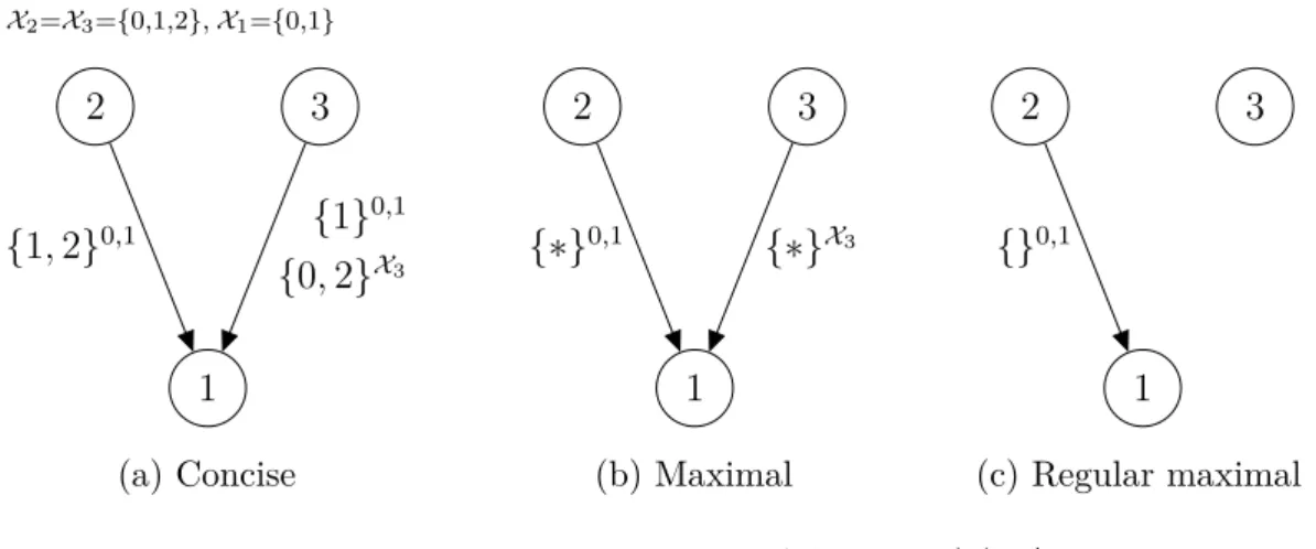
X2=X3={0,1,2},X1={0,1} 2 3 1 {1,2}0,1 {1} 0,1 {0,2}X3 (a) Concise 2 3 1 {∗}0,1 {∗}X3 (b) Maximal 2 3 1 {}0,1 (c) Regular maximal Figure 9: Regular maximal condition for PLDAGs. In (b) ’*’ denotes that an arbitrary value of the variable in question can be chosen. The empty brackets in (c) are used as there are no other parents.
Proof. A local CSI Xj ⊥ Xi | XL(i,j) = xL(i,j) is equivalent to a local PCSI Xj ⊥
Xi | Xi ∈ Xi, XL(i,j) = xL(i,j). Since all local CSIs represented by the PLDAG are explicitly included in the labels of GP L by the maximality condition they are
therefore also explicitly included in the underlyingGL and no additional local CSIs
can be induced from these labels. It follows that the underlying LDAG represents all and only those local CSIs represented by the PLDAG.
Note that an underlying LDAG of a maximal PLDAG is always a maximal LDAG. However the contrary is not always true, i.e. a maximal LDAG projected as PLDAG is not necessarily maximal.
Next the regularity condition is introduced for PLDAGs. Definition 11. Regular Maximal PLDAG
A maximal PLDAG GP L = (V, E,LDE) is regular if L(i,j) is a strict subset of XL(i,j) for all L(i,j) ∈ LE in the underlying LDAG GL= (V, E,LE).
Consider Figure 9 where all the three PLDAGs represent the same dependency structure. The PLDAG in the subfigure 9a contains labelings which induce a local CSI X1 ⊥ X3 | X2 = 1. The corresponding maximal PLDAG where this CSI is
explicitly included in the labels is shown in subfigure 9b. The CSI label set on the edge (3,1) is now complete forming a CI X1 ⊥ X3 |X2. This CI can however also
be represented by removing the edge (3,1) from the underlying DAG, as illustrated in the subfigure 9c. Similar to LDAGs, the regular maximal condition for PLDAGs prevents this kind of local CIs being formed by the labelings and instead requires
them to be represented by removing the corresponding edge from the underlying DAG. This allows us to embed the space of all possible PLDAGs to the smaller space of regular maximal PLDAGs.
Proposition 4. The labels in a regular maximal PLDAG cannot induce a complete set of local CSIs for any edge, i.e. Xj ⊥Xi |XL(i,j) =xL(i,j) for all xL(i,j) ∈ XL(i,j).
Proof. Let GP L be a regular maximal PLDAG and GL its underlying LDAG. A
local CI corresponds to a complete set of local CSIs, i.e. Xj ⊥ Xi | XL(i,j) =xL(i,j) for all xL(i,j) ∈ XL(i,j). Because the underlying LDAG GL represents all and only those local CSIs represented byGP L by Proposition 3 it is enough to show that the
claim holds for GL. Let us then assume thatL(i,j) is a label in GL. The regularity
condition of GP L requires that there must exist x ∈ XL(i,j) \ L(i,j). The maximality condition ensures that Xj 6⊥ Xi | XL(i,j) = x. Therefore no complete set of local CSIs can exist in GL nor GP L.
In regular DAGs one can discover CIs between nodes by investigating the trails between them. If all the trails between two sets of nodes are blocked by a given set S ⊂ V they are said to be d-separated by S and the corresponding variables are conditionally independent given S. In Boutilier et al. (1996) and Pensar et al. (2013) the CSI counterpart of d-separation is defined and named as CSI-separation. As d-separation, CSI-separation provides a way to infer independencies between variables directly from the graph structure. Since CSIs require a specific context to be active, the underlying DAG of an LDAG is first modified according to the given context prior to inferring independencies. The idea is based on the observation that the local conditional distributions of the nodes can be reduced to contain local CIs when the context is suitable and local CIs can be represented by removing edges. Such modified LDAGs are called context-specific.
The main difference between CSIs and PCSIs in PLDAGs is that genuine PCSIs apply only to the direction of the edge. For example if we have an edge (i, j)∈Eand a context XL(i,j) =xL(i,j) for which it holds that Xj ⊥Xi | Xi ∈ Di, XL(i,j) =xL(i,j) then only the distribution ofXj is invariant of Xi taking on values from the domain
set Di. But as noted in the Remark 1 we cannot say anything about the reverse. There is no implication that the distribution ofXi will be invariant ofXj taking on
values from any subset ofXj, even if we would specifically instantiateXi =xi with
somexi ∈ Xi. Consequently when investigating PCSI-separation between two sets of
and cannot reflect them with a removal of an edge.
The next definitions take into account the previous observations in generalizing the concept of context-specific LDAGs in Pensar et al. (2013). We begin by first providing a way to distinguish edges with PCSIs that are active in a given context and domain. The following additional notations are used. LetA, B ⊆V = (1, . . . , d) and letxB = (xbi)
k
i=1,k =|B|be a value taken byXB. ThenxB∩A is a subsequence
of xB where all elements xbi are removed if bi 6∈ A. Sequence xB∩A is then an
outcome of variable XA∩B acquired by truncating xB. Now let XA∗ ⊆ XA. Then X∗
A∩B = {xA∩B | xA ∈ XA∗} is a set of truncated elements of XA∗. Let then A
and B be disjoint and XB∗ ⊆ XB. The product XA∗ × XB∗ = {xA∪B | x(A∪B)∩A ∈ X∗
A, x(A∪B)∩B ∈ XB∗} forms a space of outcomes of XA∪B acquired by combining
elements from X∗
A and X
∗
B.
Definition 12. Satisfied label
Let GP L = (V, E,LDE) be a regular maximal PLDAG and let XC = xC be a
con-text where C ⊂ V. In the context XC = xC a label L
Di (i,j) ∈ L D E is satisfied if {xC∩L(i,j)} × XL(i,j)\C ⊆ L Di
(i,j). Let also B ⊂ V, B∩C = ∅ and let X
∗
B ⊆ XB be a
restricted domain of B. In the context XC = xC a label L
Di (i,j) ∈ L D E is satisfied in X∗ B if {xC∩L(i,j)} × X ∗ B∩L(i,j) × XL(i,j)\(C∪B)⊆ L Di (i,j).
Basically satisfied labels are labels which will include PCSIs that can be active in the given context. Local CSIs in satisfied labels will always be active as their domain contains the whole outcome space of the corresponding parent. Genuine PCSIs on the other hand require also the parent variable to be restricted to a proper domain in order to be active.
Definition 13. Active label
LetGP L = (V, E,LDE) be a regular maximal PLDAG and letB andC be two disjoint
subsets ofV, XC =xC a context and XB∗ a restricted domain of B. A satisfied label
inX∗ B, L Di (i,j)∈ L D E, is called active if Di =Xi orXi∗ ⊆ Di.
It is important to note that the conciseness condition of PLDAGs together with the Definition 12 ensures that only one label on an edge can be active at a time.
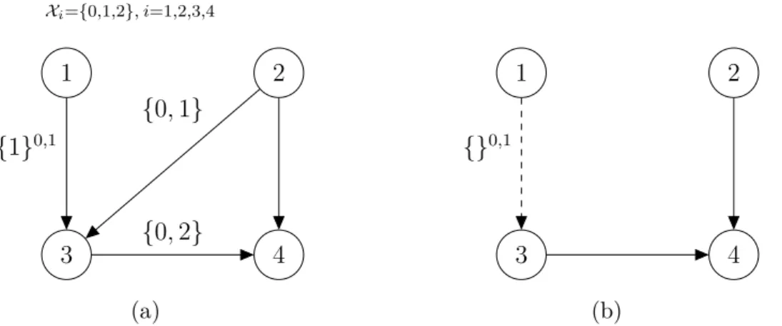
Xi={0,1,2}, i=1,2,3,4 1 2 4 3 {1}0,1 {0,1} {0,2} (a) 1 2 4 3 {}0,1 (b)
Figure 10: A PLDAG (a) and its context and domain -specific PLDAG (b) in the context X2 = 1 and restricted domain XB∗ = {0,1}, where B = {1}. The
PCSI-active edge is marked here with a dashed line.
Definition 14. Context and domain -specific PLDAG
LetGP L = (V, E,LDE) be a regular maximal PLDAG, B and C two disjoint subsets
of V, XC =xC a context and XB∗ ⊆ XB a restricted domain of B. The context and
domain -specific PLDAG of GP L is denoted by GP L(xC,XB∗) = (V, E \E
0,LD
E∗\E0),
where E∗ = {(i, j) ∈ E : LDi
(i,j) ∈ L
D
E is active} includes all the active labels and
E0 ={(i, j)∈E∗ :Di =Xi forLD(i,ji) ∈ L
D
E}the active CSI-labels. IfL(i,j)is reduced
inGP L(xC,XB∗) for some edge (i, j) because of the removal of the edges in E
0, then
the corresponding element xL(i,j) ∈ L
D
E∗\E0 is truncated accordingly. The edges in
E∗\E0 are called PCSI-active.
The edges inE∗\E0 contain the active genuine PCSI labels. These edges remain in the context and domain -specific PLDAG with their active labels. All other labels are removed. In this respect the definition of context and domain -specific PLDAG differs from the definition of context-specific LDAG where unsatisfied (and therefore inactive) labels remained in the label set. The reason for the difference is that the direction of the PCSI-active edges is essential in investigating PCSI-separation of the variables and equivalence of two distinct PLDAGs. Therefore these edges must remain in the graph. Their labels serve the purpose of marking these edges as PCSI-active. An example of a context and domain -specific PLDAG can be found from Figure 10.
Definition 15. PCSI-separation in PLDAGs
LetGP L = (V, E,LDE) be a regular maximal PLDAG,A, B, C, Sfour disjoint subsets
denoted by
XA⊥XBkGP LXB ∈ X
∗
B, XC =xC, XS,
if every trail fromXBtoXAis either blocked byXS∪C or goes through a PCSI-active
edge in the context and domain -specific PLDAG GP L(xC,XB∗).
Conjecture 5. PCSI-separation implies PCSI.
Proof. An outline of a possible proof of the conjecture. If all the trails from B to
A are blocked by XS∪C we have the case of CSI-separation considered for example
in Boutilier et al. (1996); Koller and Friedman (2009); Pensar et al. (2013). Let (xA, xS) ∈ XA× XS. Now the definition of PCSI requires that p(XA =xA | XB =
xB, XC = xC, XS = xS) = p(XA = xA | XB = x0B, XC = xC, XS = xS) for all
xB, x0B ∈ XB∗. The idea relies on the observation that restricting variables in B to
the outcome space X∗
B instead of XB makes the CPDs of the local structures in the
factorization (1) behave in a similar manner as if the active-PCSIs were active-CSIs. The requirement for every non-blocked trail from XB toXA to go through a
PCSI-active edge ensures then that computingp(XA=xA|XB =xB, XC =xC, XS =xS)
with the help of factorization (1) stays invariant when xB takes on values from X∗
B.
Conjecture 5 states that all PCSI-separations extracted from a PLDAG will imply PCSI between the corresponding variables as long as the joint distribution of the variables conforms to the PLDAG. Therefore the definition is useful for extracting independencies directly from the graph. Unfortunately the contrary is not always true. It was found in the case of CSI-separation that there are certain situations where there exists independencies between sets of variables which were not CSI-separated by definition (Koller and Friedman, 2009). They arise from multiple labels combined and require other means such as reasoning by cases to be recovered. Since the definition of PCSI-separation is based on the definition of CSI separation, it is subject to the same limitation.
As mentioned before the factorization of the joint distribution (1) resulting from local Markov property requires a conforming joint distribution p to be definable through the local structures of a DAGG. This corresponds to a set of CIs that have to be in effect in p. The CPTs of the local structures have no further restrictions imposed by Galthough some parameterizations result in additional independencies not represented by G. If G encodes exactly the same CIs that are also in effect in the given distribution p, it is then said that G is faithful to p. If also G0 encodes
the same set of CIs, they are called Markov equivalent. In this case it is possible to factorize palong both G and G0.
PLDAGs and LDAGs add restrictions for the CPTs of the nodes. A label on an edge corresponds to a simple local CSI or PCSI which must be implemented in the corresponding CPT. The number of parameterizations for PLDAGGP L is therefore
smaller compared to its underlying DAG G. Likewise to Markov equivalence of DAGs, two PLDAGs GP L and G0P L are said to be PCSI-equivalent, if they encode
the same PCSIs structure. Note that both CSI and CI are special cases of PCSI. Next we define PCSI-equivalence formally and then proceed in investigating char-acteristics of PCSI-equivalent PLDAGs.
Definition 16. PCSI-equivalence for PLDAGs
Let GP L = (V, E,LDE) and G
0
P L = (V, E
0,L0A
E0) be two distinct regular maximal
PLDAGs. The PLDAGs are said to be PCSI-equivalent ifI(GP L) = I(G0P L), where I(·) denotes the dependency structure represented by a PLDAG. A set containing all PCSI-equivalent PLDAGs forms a PCSI-equivalence class.
Proposition 6. Let GP L = (V, E,LDE)and G
0
P L = (V, E
0,L0A
E) be two regular
maxi-mal PLDAGs belonging to the same PCSI equivalence class. Their underlying DAGs
G= (V, E) and G0 = (V, E0) must then have the same skeleton. Proof. Let us assume thatGP L = (V, E,LDE) andG
0
P L = (V, E
0,L0A
E) are two regular
maximal PLDAGs belonging to the same PCSI equivalence class, but that they do not have the same skeleton. There must then exist an edge in one of the two PLDAGs that does not exist in the other. Let us assume that (i, j)∈ E but (i, j) ∈/ E0 and (j, i)∈/ E0. Now it holds thatXi 6⊥Xj |XS for allS ⊆V \ {i, j}inGP L because the
trail from i toj cannot be blocked and GP L is regular maximal. Because of
PCSI-equivalence, there must then exist an S-active trail between i and j in GP L0 with
everyS ⊆V \{i, j}. That means thatXi has to be inXj:s markov blanket. Because
there is no edge between them in GP L0,Xi has to be then another parent of a child
of Xj. This means that Xi ⊥Xj |ΠGP L
0
j inGP L0 and therefore in GP L as well. But
this is a contradiction with the observation Xi 6⊥Xj |S for all S ⊆V \ {i, j} made
earlier. They then must have the same skeleton.
The next proposition provides a correspondence between concepts of PCSI-equivalence and Markov-equivalence.
Proposition 7. Let GP L = (V, E,LDE) and G0P L = (V, E,L0AE0) be two
PCSI-equivalent regular maximal PLDAGs. Their context-specific PLDAGs GP L(xV,∅)
and G0P L(xV,∅) must then be Markov equivalent for all xV ∈ XV.
Proof. LetGP L = (V, E,LDE) andG
0
P L = (V, E
0,L0A
E0) be two context-specific regular
maximal PLDAGs. Let G(xV,∅) and G0(xV,∅) respectively denote the underlying
DAGs of their context-specific PLDAGsGP L(xV,∅) andGP L0 (xV,∅) for allxV ∈ XV.
AsGP LandG0P Lare PCSI-equivalent they must therefore encode also the same CSIs.
Assume then that there exists a joint outcome xV ∈ XV for which the underlying
DAGs G(xV,∅) and G0(xV,∅) are not Markov equivalent, i.e. they have different
(1) skeletons or (2) immoralities. (1) If they have different skeletons, there exists an edge {i, j} in, say, the skeleton of G(xV,∅) but not in the skeleton of G0(xV,∅).
Due to Proposition 6, the underlying DAGs G and G0 must nevertheless have the same skeleton. The lack of the edge inG0(xV,∅) implies that a local CSI of the form
Xj ⊥ Xi | XL(i,j) = xL(i,j) holds in G
0(x
V,∅) but not in G(xV,∅). (2) Assume that
there exists an immoralityi→j ←k in, say,G(xV,∅) but not inG0(xV,∅). If there
is no edge betweeniandk inGP L (andG0P L) there must exist someS ⊆V \ {i, j, k}
for which Xi ⊥XkkGP LXS. Consequently Xi ⊥Xk |XS is represented byGP L but
not by G0P L because there exists at least one active trail between Xi and Xk via
Xj. If there exists an edge between i and k in GP L (and G0P L), there must exist
a local CSI of the form Xi ⊥ Xk | XL(k,i) = xL(k,i) (or Xk ⊥ Xi | XL(i,k) = xL(i,k)) that holds in G0P L where j ∈ L(k,i) (or j ∈ L(i,k)). But the same cannot hold in
GP L since setting Xj =xj will activate the trail betweenXi and Xk viaXj inGP L.
(1) and (2) allow us to conclude that the CSI-dependency structures represented by
GP L and GP L are different which contradicts the assumption of them being
PCSI-equivalent. Therefore G(xV,∅) and G0(xV,∅) must be Markov equivalent for all
contextsxV ∈ XV.
The characteristics in Propositions 6 and 7 are the same as for LDAGs in Pensar et al. (2013). The latter proposition provides an interesting special case as noted by Pensar et al. (2013) when there exists a joint outcome xV for which no label is
satisfied. This condition provides a more strict version of Proposition 6 as stated in the next Corollary.
Corollary 8. Let GP L = (V, E,LDE)andG
0
P L = (V, E,L
0A
E0) be two regular maximal
PLDAGs that are PCSI-equivalent and let their labelings be such that there exists at least one joint outcome xV ∈ XV for which no label is satisfied. The underlying
Proof. This Corollary is a direct consequence of Proposition 7.
The next proposition investigates differences with respect to genuine PCSI-labels between two PCSI-equivalent PLDAGs. Remark (1) suggests that a single edge with a genuine label cannot be reversed while maintaining the same PCSI-encoding. This observation is formalized in the next proposition.
Proposition 9. Let GP L = (V, E,LDE) be a regular maximal PLDAG and let an
edge (i, j) ∈ E have a genuine PCSI-label LDi
(i,j) ∈ L D E and let G 0 P L = (V, E 0,L0A E0)
where E0 = (E\ {(i, j)})∪ {(j, i)}. Then GP L and G0P L cannot be PCSI-equivalent.
Proof. LetGP L = (V, E,LDE) be a regular maximal PLDAG and let an edge (i, j)∈
E have a genuine PCSI-label LDi
(i,j) ∈ L D E, G 0 P L = (V, E 0,L0A E0) where E0 = (E \
{(i, j)})∪ {(j, i)} and let xi, x0i ∈ Di. Let us assume that GP L and G0P L are
PCSI-equivalent. Denote C = L(i,j) where L(i,j)∪ {i} = Πj with respect to GP L and let
XC = xC be a context where xC ∈ LD(i,ji). Now p(Xj = xj | Xi = xi, XC = xC) =
p(Xj =xj |Xi =xi0, XC =xC) holds in GP L by the definition and must hold inG0P L
with all its parameterizations in order for them to be PCSI-equivalent. Because the edges inGP LandG0P Lare directed the same way except for the edge between nodesj
andiit follows that all nodes inCare either parents or non-descendants ofjinG0P L. Otherwise there is a cycle inG0P L. Furthermore j cannot have any other parents in the context-specific PLDAGG0P L(xC,∅) except foriand nodes inC. Otherwise there
is either a cycle inGP L or the context-specific PLDAGsGP L(xC,∅) andG0P L(xC,∅)
are not Markov equivalent, violating Proposition 7. Thereforep(Xi =xi |G0
P L XΠi =
xΠi) =p(Xi =xi |G0P L Xj =xj, XC =xC) holds in G
0
P L for all (xi, xj)∈ Xi× Xj and
xΠj ∈ XΠj wherexΠj includes the context configurationxC and xj. Now computing
p(Xj =xj |Xi =xi, XC =xC) in G0P L yields p(Xj =xj |Xi =xi, XC =xC) = p(Xi =xi |G 0 P L Xj =xj, XC =xC)p(Xj =xj |G 0 P L XC =xC) P xj∈Xjp(Xi =xi |G0P L Xj =xj, XC =xC)p(Xj =xj |G 0 P L XC =xC) = P p(xi |xj)p(xj) xj∈Xjp(xi |Xj =xj)p(Xj =xj) , (5)
p(Xj =xj |Xi =xi, XC =xC) = p(Xj =xj |Xi =x0i, XC =xC) is equivalent to p(xi |xj)p(xj) P xj∈Xjp(xi |Xj =xj)p(Xj =xj) = p(x 0 i |xj)p(xj) P xj∈Xjp(x 0 i |Xj =xj)p(Xj =xj) ⇐⇒ p(xi |xj) X xj∈Xj p(x0i |Xj =xj)p(Xj =xj) =p(x0i |xj) X xj∈Xj p(xi |Xj =xj)p(Xj =xj) ⇐⇒ p(xi |xj) X x∗j6=xj p(x0i |Xj =xj∗)p(Xj =x∗j) (6) =p(x0i |xj) X x∗ j6=xj p(xi |Xj =x∗j)p(Xj =x∗j).
Now there must exist x∗j ∈ Xj such that equation p(xi | xj) = p(xi | x∗j) is not
enforced by a label in G0P L. Otherwise there must be an active CSI in the context
XC =xC between nodesj and iin G0P L which contradicts the assumption of
PCSI-equivalence. Now it is possible to reparameterize G0P L so that only the probability
p(xi | x∗j) is changed in equation (6). This change will affect only the right hand
side sum in equation (6) by either decreasing or increasing the sum. This means that it is impossible for the equation to hold with both the original and modified parameterization. Therefore GP L and G0P L cannot be PCSI-equivalent.
It seems possible that a stronger version of Proposition 9 could be proved stating that all edges with genuine labels must be in the same orientation in all PCSI-equivalent PLDAGs. This would mean that the genuine PCSI-labels would have to be practically the same in all PCSI-equivalent PLDAGs. Nevertheless, when investigating PCSI-equivalence of two distinct PLDAGs one can to first check the conditions from Propositions 6 and 7. As suggested in Pensar et al. (2013) it often suffices to compare context-specific graphs for only a subset of variables since not all contexts will affect the structure of the graph. Furthermore, all outcomes for which no labels in either of the graphs are satisfied need only to be checked once as the context-specific graphs in all these cases are equal to the underlying DAG. The last thing left is to compare the genuine PCSI-labels one by one. If they are practically the same, i.e. active in the same context and domain in both of the PLDAGs, then with the help of the next Proposition the PLDAGs must be PCSI-equivalent. Proposition 10. Let GP L = (V, E,LDE) and G0P L = (V, E,L0AE) be two regular
Markov-equivalent for all xV. If there exists distributions P and P0 such that I(GP L) = I(P) and I(GP L0 ) = I(P0) and both GP L and G0P L have the same
gen-uine PCSI-labels, i.e. they are active in the same context and domain in both of the PLDAGs, then GP L and G0P L must be PCSI-equivalent.
Proof. Let GP L = (V, E,LDE) and G0P L = (V, E0,L0AE) be two regular maximal
PLDAGs. Let G(xV,∅) and G0(xV,∅) respectively denote the underlying DAGs of
their context-specific PLDAGs GP L(xV,∅) and G0P L(xV,∅). Assume that G(xV,∅)
and G0(xV,∅) are Markov equivalent for all xV ∈ XV. Let P be a distribution for
which GP L is a perfect PCSI-map. Each joint probability p(XV = xV) factorizes
according toG(xV,∅). Since G(xV,∅) and G0(xV,∅) are Markov equivalent, we can
refactorize each joint probability p(XV = xV) according to G0(xV,∅) without
al-tering the joint distribution or inducing any additional dependencies. Because the genuine labels are the same in both of the PLDAGs the edges with PCSI-active labels must be the same and in the same orientation and therefore encode the same PCSI-structure in the corresponding CPDs of the local structures. This means that G0P L is also a perfect PCSI-map of P. Since I(GP L) =I(P) =I(G0P L)
3
Bayesian learning of PLDAGs
This section closely follows the corresponding section in Pensar et al. (2013) due to the similarity of structure learning between LDAGs and PLDAGs. First the Bayesian approach is briefly described after which the structure learning alogrithm is given. The last part describes a cross-validation method for choosing an initial parameter for the scoring function.
3.1
Bayesian scoring function
Let X = {xi}ni=1 denote a set of training data consisting of n observations xi =
{xi1, . . . , xid}of the variables{X1, . . . , Xd}such that xi ∈ X. A PLDAG is denoted
by GP L and GP L denotes the set of all regular maximal PLDAGs. The
underly-ing DAG is denoted by G and its model space by G. The outcome space XΠj of
the parents of node Xj is partitioned according to the PCSIs in GP L, so that each
part in the partition has a separate conditional distribution over the child node Xj.
This partition of XΠj is denoted by SΠj = {Sj1, . . . , Sjkj}, where kj is the number
of classes |SΠj|. The notations rj = |Xj| and qj = |XΠj| denote the cardinality of
the outcome space of variableXj and its parentsXΠj respectively. The conditional
probability distribution of Xj given the class Sjl is defined by the parameter
vec-tor θjl = (θ1jl, . . . , θrjjl). The whole parameter space induced by GP L is denoted
by ΘGP L and the number of free parameters spanning the parameter space with
dim ΘGP L. An instance θ∈ΘGP L contains the parameters defining the specific joint
distribution that factorizes according to the PLDAG GP L. The parametrization of
PLDAGs is thus similar to parametrization of LDAGs. Finally, we use n(xij ×Sjl)
to denote the total count of configurations xij×Sjl inX.
In the Bayesian approach to model learning, one considers the posterior distribution of the models given some data,
p(GP L |X) =
p(X|GP L)p(GP L)
P
GP L∈GP Lp(X |GP L)p(GP L)
. (7)
Here p(X | GP L) is the marginal likelihood of observing the data X given the
model GP L ∈ GP L and p(GP L) is the prior probability for the given model. The
denominator is a normalizing constant that does not depend on GP L and can thus
be ignored when comparing posterior probabilities of different PLDAGs. These unnormalized posterior probabilities will be used as scores for the PLDAGs given
data X and therefore our main interest is to find the maximum a posteriori model, i.e. the solution to
arg max
GP L∈GP L
p(X |GP L)p(GP L). (8)
For each PLDAG there are many possible generating distributions, i.e. instances
θ ∈ ΘGP L, conforming to the independence structure represented by the PLDAG.
In order to evaluatep(X|GP L) one needs to consider all of the possible
parameter-izations and weight them with respect to a prior according to
p(X |GP L) =
Z
θ∈ΘGP L
p(X |GP L, θ)f(θ |GP L), (9)
where f(·|GP L) denotes the parameter vector prior conditioned on the model.
Using a product of Dirichlet distributions as the prior in equation (9) allows it to be solved analytically for regular Bayesian Networks as introduced and discussed in Cooper and Herskovitz (1992). The likelihood is called the Cooper-Herskovitz likelihood. Pensar et al. (2013) uses a modified version of this likelihood from the works of Friedman and Goldszmidt (1996) and Chickering et al. (1997) for CPT-trees and decision graphs respectively, as they partition the parental outcome spaces in similar manner to LDAGs. The same idea can be further directly applied to PLDAGs leading to the expression
p(X|GP L) = d Y j=1 kj Y l=1 Γ(Prj i=1αijl) Γ(n(Sjl) +P rj i=1αijl) rj Y i=1 Γ(n(xji×Sjl) +αijl) Γ(αijl) (10) wheren(·) is the count defined earlier and theαijl:s are the hyperparameters defining
the collection of Dirichlet prior distributions for the parameters of the joint distri-bution. The only difference to the original Cooper-Herskovitz likelihood is that the separate parental configurations are replaced with the classes Sjl.
In order to calculate (10) the prior parameters αijl have to be specified for the
conditional probability distributions (CPDs). The prior parameters reflect our initial belief about the CPDs. Buntine (1991) defines a non-informative prior for ordinary Bayesian Networks which was extended to be used with LDAGs in Pensar et al. (2013). The idea behind this non-informative prior is that each joint outcome is equally likely for the prior thus ensuring that equivalent networks are evaluated equally by the marginal likelihood. We use the same extension here and define the
parameters for the Dirichlet priors as
αijl =
N rj·qj
|Sjl| (11)
for each i = 1, . . . , rj where the number of parent configurations qj is with respect
to the underlying DAG and |Sjl| denotes the number of states of XΠj in Sjl. The
parameterN, known as the equivalent sample size, reflects the strength of our prior belief on the prior parameter distributions in general.
The last step left is to define a prior distribution over the set of PLDAGs. A common choice in ordinary Bayesian networks is the uniform prior which would base the scoring function on the marginal likelihood alone if (7) is used for scoring. Uniform prior is shown to work quite well for ordinary DAGs but Pensar et al. (2013) discovered that with LDAGs the model prior needs to be given more attention. They noticed that with LDAGs the marginal likelihood alone has a tendency to overfit the dependency structure for limited sample sizes by favoring dense graphs with complex labelings. Although the marginal likelihood of such models is increased they are more prone to contain false dependencies and thereby fail to capture the true global dependency structure. This has then direct negative effect for example on their out-of-sample predictive performance. Dense graphs with complex labelings can also be seen as moving the encoding of the dependency structure from the underlying DAG structure to the labels. This is basically against the fundamental idea of modularity on which the concept of graphical models is based on. This same overfitting phenomenon holds true for PLDAGs also as can be seen in the results section.
In order to control this Pensar et al. (2013) introduce a model prior which penalizes the excessive use of labels in the learned model by comparing the number of free parameters in the learned LDAG and its underlying DAG. The absolute value of the difference directly reflects the number of labels used and can be used to penalize the score. This same idea can be used with PLDAGs, since the only difference is that there is more variety in the possible labels that can be attached to the graph. Every added label nevertheless increases the difference in the number of free parameters according to the size of the domain of the label. Following Pensar et al. (2013) the model prior is defined as
p(GP L)∝κdim(ΘG)−dim(ΘGP L)= d
Y
j=1