Modelling and Forecasting Noisy Realized Volatility

(1)

Modelling and Forecasting Noisy Realized Volatility*

Manabu Asai

Faculty of Economics Soka University, Japan

Michael McAleer

Econometric Institute Erasmus School of Economics Erasmus University Rotterdam

and Tinbergen Institute

The Netherlands and

Department of Quantitative Economics Complutense University of Madrid

Marcelo C. Medeiros

Department of Economics

Pontifical Catholic University of Rio de Janeiro

Revised: April 2011

* The authors are grateful to Marcel Scharth for efficient research assistance, and to an associate editor and an anonymous referee for helpful comments and suggestions. For financial support, the first author acknowledges the Japan Society for the Promotion of Science and the Australian Academy of Science, the second author acknowledges the Australian Research Council, the National Science Council, Taiwan, and the Japan Society for the Promotion of Science, and the third author wishes to acknowledge CNPq, Brazil.

(2)

Abstract

Several methods have recently been proposed in the ultra high frequency financial literature

to remove the effects of microstructure noise and to obtain consistent estimates of the

integrated volatility (IV) as a measure of ex-post daily volatility. Even bias-corrected and

consistent realized volatility (RV) estimates of IV can contain residual microstructure noise

and other measurement errors. Such noise is called “realized volatility error”. As such errors

are ignored, we need to take account of them in estimating and forecasting IV. This paper

investigates through Monte Carlo simulations the effects of RV errors on estimating and

forecasting IV with RV data. It is found that: (i) neglecting RV errors can lead to serious

bias in estimators; (ii) the effects of RV errors on one-step ahead forecasts are minor when

consistent estimators are used and when the number of intraday observations is large; and

(iii) even the partially corrected R2 recently proposed in the literature should be fully corrected for evaluating forecasts. This paper proposes a full correction ofR2. An empirical example for S&P 500 data is used to demonstrate the techniques developed in the paper.

Keywords: realized volatility; diffusion; financial econometrics; measurement errors;

(3)

1 Introduction

Given the rapid growth in financial markets and the continual development of new and more complex financial instruments, there is an ever-growing need for theoretical and empirical knowledge of volatility in financial time series.

There is, however, an inherent problem in using models where the volatility measure plays a central role. The conditional variance is latent, and hence is not directly observable. It can be estimated, among other approaches, by the (Generalized) Autoregressive Conditional Heteroskedasticity, or (G)ARCH, family of models proposed by Engle (1982) and Bollerslev (1986) or stochastic volatility (SV) models (see, for example, Taylor (1986)). McAleer (2005) provides a exposition of a wide range of volatility models, and Asai, McAleer and Yu (2006) for a review of the growing literature on multivariate SV models.

More recently, Andersen and Bollerslev (1998) showed that ex post daily volatility is best measured by aggregating 288 squared five-minute returns. The five-minute frequency was suggested as a trade-off between accuracy, which is theoretically optimized using the highest possible frequency, and microstructure noise that can arise through the bid-ask bounce, asynchronous trading, infrequent trading, and price discreteness, among other factors.

Ignoring the remaining measurement error, the ex post volatility essentially becomes “observable”, and hence it can be modelled directly, rather than being treated as a latent variable. Based on the theoretical results of Barndorff-Nielsen and Shephard (2002), Andersen, Bollerslev, Diebold and Labys (2003) and Meddahi (2002), several recent studies have documented the properties of realized volatility constructed from high frequency data. However, it is well known that neglecting microstructure noise in calculating realized volatility (RV) can lead to biased and inconsistent estimates of integrated volatility (IV) as a true measure of daily volatility.

(4)

financial literature to remove the effects of microstructure noise and to obtain consistent estimates of the IV (see Barndorff-Nielsen, Hansen, Lunde and Shephard (2008), Christensen, Oomen and Podolskij (2008), Hansen, Large and Lunde (2008), and Zhang, Mykland and Aït-Sahalia (2005)). For an extensive review of the realized volatility literature, see McAleer and Medeiros (2008) and Bandi and Russell (2007).

Nevertheless, even bias-corrected and consistent realized volatility estimates of the IV can contain residual microstructure noise and other measurement errors that should not be ignored. Furthermore, the consistency of the above mentioned estimators is derived under some (strong) assumptions about the microstructure noise. Whenever some of these assumptions are not met in practice, the estimators turn to be inconsistent. Finally, if the number of intraday observations is small (due to illiquidity effects or data availability), the remaining measurement error may not be negligible. Barndorff-Nielsen and Shephard (2002) refer to such remaining noise as the “realized volatility (RV) errors”. They suggested a method to estimate the continuous-time SV model, in which volatility follows a non-Gaussian Ornstein-Uhlenbeck (OU) process (see also Corradi and Distaso (2006) for a discussion of measurement errors and realized volatility).

The contribution of this paper is two-fold. First, we extend Barndorff-Nielsen´s and Shephard (2002) approach and estimate three different models of IV. The common features between Barndorff-Nielsen and Shephard (2002) and the current paper is the use of state space representation to remove such RV errors. This paper deals with discrete-time SV models, in which the logarithm of IV follows a K-component model, a long memory model (ARFIMA), or a heterogeneous autoregressive (HAR) model. Our

K-component model corresponds to the continuous-time SV model of Chernov et al. (2003). Monte Carlo simulation experiments are presented to investigate the effects of the RV errors on the estimators and forecasts of these three models. Second, we show that, in the presence of RV errors, the R2 correction proposed by Andersen, Bollerslev and Meddahi (2005) is only a partial correction. We provide a corrected R2 measure in Mincer-Zarnowitz regressions when the dependent variable is a noisy RV measure.

(5)

serious bias in estimating IV, and that the new method can eliminate the effects of the errors. Finally, the fully corrected R2 proposed in this paper is needed in most cases.

The plan of the remainder of the paper is as follows. Section 2 discusses the effects of RV error on estimating and forecasting IV. Section 3 presents the results of Monte Carlo simulation experiments regarding the effects of RV error, using the

K-component, long memory and HAR models. Section 4 proposes a new method to fully correct R2 in the presence of RV error. The results of an empirical example are analyzed in Section 5. Some concluding remarks are given in Section 6.

2 Realized Volatility and the Significance of Measurement Errors

Suppose that, along day t, the logarithmic prices of a given asset follow a continuous time diffusion process:

 , 2 , 1 , 1 0 ), ( ) ( ) ( ) (t  t d  t dW t   t dp         ,

where p(t) is the logarithmic price at time t , (t) is the drift component, (t) is the instantaneous volatility (or standard deviation), and

) (t

W is a standard Brownian motion. In addition, suppose that (t) is orthogonal to W(t), such that there is no leverage effect. This assumption is standard in the realized volatility literature.

Andersen, Bollerslev, Diebold and Labys (2003) and Barndorff-Nielsen and Shephard (2002) showed that daily returns, defined as rt  p(t) p(t1), are Gaussian

conditionally on _t 



(t1),(t1)



__1₀ , the -algebra (information set) generated by the sample paths of (t1) and (t1), 01, such that

      _ _ _ _ 



1 0 2 1 0 ( 1) , ( 1) , N ~  t  d  t  d r_t _t . The term 2 1 2 0 ( 1) t

IV 



 t  d is known as the integrated variance, which is a measure of the day-t ex post volatility. The integrated variance is typically the object of interest as a measure of the true daily volatility.

(6)

In general, 



t

(7)

where u_t is assumed to be an independent process with mean 0, variance u2 ,

and E(ut |IVt)0

2

. Hereafter, u_t ~ID(0,_u2). We call the second term in (1), u n_t _t , the “realized volatility error”. It should be noted that u_t is not, in principle, the microstructure noise, as it is just the estimation error.

The approach proposed in this paper is based on equation (1), which shows that the last term plays a key role as a measurement error. It is known that measurement errors can lead to serious bias in estimating econometric models. As the logarithm of

t

RV is modelled in the literature, it is useful to consider the measurement error of

lnRVt when it is based on equation (1). By using a Taylor series expansion of







can be a linear or nonlinear function, and _t is the innovation term. This model includes ARMA and ARFIMA models, by the AR

 

 representation, assuming that the invertibility conditions are satisfied. Obviously, it also

2

We only assume this for the purpose of describing the idea. We may relax this assumption, as in

Barndorff-Nielsen and Shephard (2002), allowing the variance of u_t to depend on t, and u_t to be

(8)

contains the non-linear AR models. Then we have the model of RV_t as





1 1 1 (1 ) t t , t d t t   L w g X W

 with the function







 

 

 







 

 

 







1 1 1 , 1 ln , 1 ln , 1 ln , 1 ln , , d d t t t t t t d d t t g X W g L RV w L RV w g L RV L RV                     

and X_t 



lnRV_t, lnRV_t_₁,



and W_t 



w w_t, _t_₁,



. This leads to a measurement error problem in nonlinear regression models. Estimation neglecting measurement errors produces bias in the estimators, which may affect the bias in the forecasts. Such bias depends both on the model and the size of the RV error.

Consider two examples. If the true ln

 

t follows an OU process, then lnIV_t follows an AR(1) process, namely lnIV_t_₁  



1   



 lnIV_t_t. Then we have a model of RV_t as lnRV_t_₁ 



1   



 lnRV_t_t_₁ , where

1 1

t t wt wt

_   _  . Note that _t_₁ is correlated with RV_t, by the structure of the model. Hence, neglecting w_t_₁w_t causes a familiar problem of measurement errors in regression models. The OLS estimator for  is biased due to the RV error in RV_t

and the correlation between lnRV_t and the disturbance. On the other hand, taking

account of w_t_₁w_t leads to an ARMA(1,1) specification of lnRV_t, as an AR(1) plus noise follows an ARMA(1,1) model, in general. In the case of taking account of w_t, the

forecast of lnRV_t is made of all the past information, lnRV_t_₁, lnRV_t_₂, , due to the

(9)

measurement errors, the forecast of lnRV_t depends only on lnRV_t_₁ from the AR(1) specification. Hence, forecasts that neglect the measurement errors lead to two kinds of bias, one caused by the bias in the estimate of , and the other from the lack of information.

Another example is the Heterogeneous Autoregressive (HAR) model of Corsi (2009). Consider the HAR model of lnIV_t as

.

In this case, ln RVt follows a restricted ARMA(22,22) model. Neglecting the effects of wt and using QML lead to bias in the estimates of the parameters. Furthermore, forecasts obtained by neglecting measurement errors will be biased due to the bias in the estimates and the lack of information. Overall, the moving average term caused by measurement error plays an important role in estimating and forecasting IV.

3 Effects of RV Errors

In the following section, we will investigate the effects of the RV error on estimating and forecasting volatility models. We consider three kinds of models, namely the K-component, long memory and HAR models, which are familiar in empirical analysis. Then we will conduct Monte Carlo simulations using two quasi-maximum likelihood (QML) estimators, one taking account of measurement errors caused by RV error, and another which neglects measurement errors. The purpose of the simulations is to (i) compare the finite sample properties of two estimators, (ii) investigate differences in forecasts based on these estimators, and (iii) check the effects on the corrected R2 values.

(10)

3.1 K-component Model

With regard to IV_t, consider the following K-component model:

1 , 1 exp , , 1, , , K t it i i t i it i it IV i K            _ _     



(4)

where _it follows the independent standard normal distribution. In the literature of stochastic volatility based on observed return series, Chernov et al. (2003) and Asai (2008), among others, consider such a K-component model in a more general framework. Here, we will consider estimation of the model via a proxy for the latent IV, namely realized volatility.

Based on equations (1)-(4), we have

1 ln ln ln K t t t it t i RV IV w   w     



 . (5)

Thus, we can construct the state space model with the measurement equation (5) and the state equation of _it, which enables an application of the QML method via the Kalman

filter. Note that the distribution of the measurement error, w_t, is unknown.

We may have filtered (or smoothed) the estimate of the logarithm of integrated volatility via the Kalman filter (or smoother). For purposes of forecasting out of sample,

the one-step ahead predicted value, _, ₁

1 ˆ

ˆ

ln K _{i T}

i





_ _ , is also available. The method here includes estimation of the K-component model in the absence of RV errors. Let

w

 be the standard deviation of w_t. By setting _w0, the approach can deal with the case of no measurement errors.

(11)

3.2 Long Memory Model for Integrated Volatility

In this section we consider a long memory model for the logarithm of IV. For convenience, we assume that IV_t exp

 

x_t and that x_t follows an ARFIMA(p,d,q) model. Then we have



  

 

ln ln ln , 1 , t t t t t d t t RV IV w x w L L x L            (6)

where t ~N



0,2



and wt is defined by equation (2). The spectral density of the

model is given by

 

2 2 ₂ 2 2 ₂ , 2 1 i w d i i e f e e       _                 .

Thus, we may apply the method of Breidt, Crato and de Lima (1998) in order to estimate the above model3. With an adaptation of the algorithm given in Harvey (1998), we can obtain the estimates and forecasts of lnIV_t. In order to estimate the

model without RV errors, we need only to set w to zero.

3.3 HAR Model forIntegrated Volatility

We consider the HAR model for IV as

5 22 1 1 2 1 3 1 1 1 ln ln ln , 1 1 ln ln ln ln , 5 22 t t t t t t t t i t i t i i RV IV w x w x x x x                   







 (7)

3 _{An alternative method is to work with the filtering algorithm proposed by So (1999), but}

(12)

where _t ~N



0,_2



and w_t is defined by equation (2). Note that setting





0 1 2 3

exp 1

  _    _ and x_t lnIV_tln leads to equation (3). As the model is an AR(22) plus noise, we can use the QML method via the Kalman filter. For purposes of forecasting, the one-step ahead predicted value is also available from the Kalman filter. For the case of neglecting measurement error, we may handle the case by setting _w 0. In this case, the QML estimator is equivalent to the OLS estimator.

3.4 Framework of Experiments

We start from equation (1) for specifying the magnitude of the RV error, which is assumed to be independent of IVt. The variance of the RV error is given by u2 nt2



 .

We consider the case of ZMA (2005), which indicates that 1 6. Let the variance of

t

IV be _iv2 . Then we define the variance ratio of the RV error to volatility as

2 2 u iv t ev n    . (8)

In the following, we set ev0.03 in order to consider a minor RV error compared with volatility. It should be noted that, if the RV error is large, it will lead to bias in estimating and forecasting the models of IV. Hence, we exclude the obvious case in order to concentrate on the case that the estimator of RV is consistent and well-behaved.

In the following Monte Carlo simulations, we generate data of IV_t with

sample size T+1. The parameter setting are as follows;



    1, 1, 2, 2,

 

 0.98, 0.1, 0.4, 0.4,1



for the two component model (equation (4) with

(13)



for purposes of investigating the effects of using the noisy RV as the regressand. It is important to stress that the hypothesis we want to test with the MZ regressions are the following :

(1) E(lnIVt |Allinformation up to timet-1)hˆt|t1 and

(14)

3.5 Monte Carlo Results

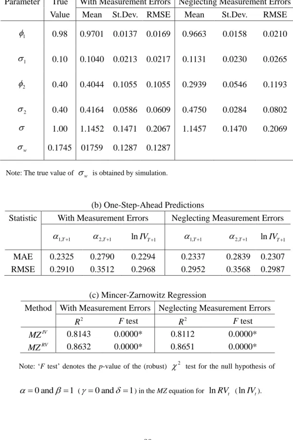
This subsection reports the results of the Monte Carlo simulations described above. Table 1(a) shows the true parameters and the mean, standard deviations and RMSE of two kinds of QML estimators for 1000 replications with T=1000. As it is not easy to obtain the true value of _w analytically, we use the simulated value from 1000 replications as a proxy. The QML estimator taking account of RV error has a small bias, while the QML estimator neglecting RV error has a relatively large bias, especially for



 2, 2



. On the other hand, introducing w makes the standard deviations for



 2, 2



larger, compared with those for the QML neglecting RV error. Overall, the

RMSE values for the QML with measurement errors are always smaller than those for the QML neglecting measurement errors.

In the above simulations, we also obtained the predicted values, ˆ_1,_T_₁, ˆ_2,_T_₁

and 2 _, ₁

1 ˆ

ˆ

ln _{i T}

i





_ _



hˆ_T__1|_T



. Table 1(b) presents the MAE and RMSE values for the predictions of _1,_T_₁, _2,_T_₁ and lnIV_T_₁. The QML estimator taking account of RV error always has smaller MAE and RMSE values than the corresponding QML estimator neglecting the RV error. Table 1(c) shows R2 and the F test for the MZIV

and MZRV regressions. The F test is for the null hypothesis H₀:0 and 1 ( 0 and 1) in the MZ equation for lnRV_t ( lnIV_t). The p-values in Table 1(c) indicate that the model is not correctly specified, implying that the test tends to over-reject the null hypothesis.

The QML estimator taking account of RV error has larger R2 than the corresponding QML estimator neglecting RV error, as expected. Interestingly, MZRV

shows the opposite result. Thus, R2 for MZRV yields a misleading result. Therefore, we must be careful in comparing R2 values based on MZRV. We will discuss this

(15)

point further in the next section.

Now we turn to the results for the ARFIMA model, which is given in Table 2. Table 2(a) presents the true parameters and the mean, standard deviations and RMSE of two kinds of QML estimators for 1000 replications with T=1000. We set _w as the simulated value from 1000 replications as given previously. In the results for QML neglecting measurement errors, the estimator for d has a downward bias, while the estimator for _ has an upward bias. The estimator for  is unbiased. In the results for QML taking account of RV error, the bias is minor, except for , but the standard deviations are relatively large. This may be explained by three reasons: (i) The sample size is relatively small for the analysis of a long memory process; (ii) the measurement error in the current parameter setting is too small to detect; (iii) As in Table 1(a), introducing _w for accommodating measurement errors make larger the standard deviations of some parameters which are strongly affected by neglecting the noise.

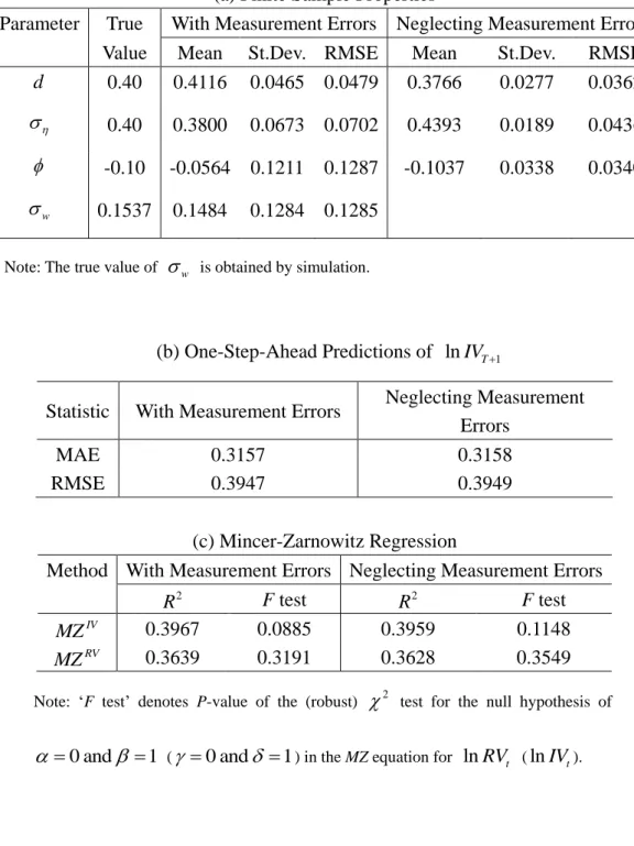
In order to investigate the effects of sample size, Table 3 reports the results for

T=2000. The bias in  for the QML accommodating the RV errors becomes smaller. In all cases, the standard deviations and RMSE are smaller than those in Table 2.

For purposes of forecasting IV, Table 2(b) shows that the QML estimator taking account of RV error always has smaller MAE and RMSE values than the corresponding QML estimator neglecting the RV error. This is the same as in Table 1(b). Table 2(c) presents R2 and the F test for the MZIV and MZRV regressions. The p-valuesof the

F test are for the null hypothesis H₀:0 and 1 ( 0 and 1) in the MZ

equation for lnRV_t ( lnIV_t), and indicate that the model is correctly specified. In both

the cases of including and neglecting RV error, MZIV has larger R2 values than does

RV

MZ . This result is reasonable, as the denominator of R2 is the sum of squared deviations of the regressand, for which lnIVt has smaller values than does lnRVt.

(16)

values than the corresponding QML estimator neglecting the RV error. We obtain the same conclusions from Tables 3 (b) and 3(c) for T=2000.

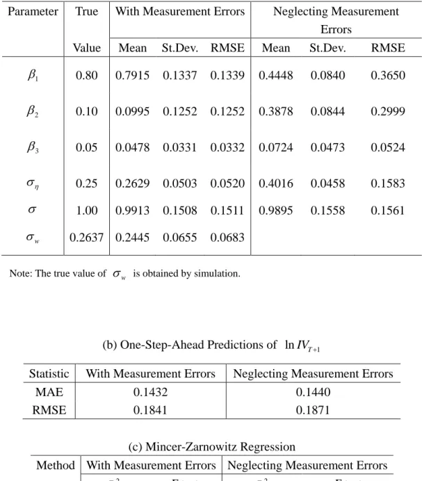
Third, we discuss the simulation results of the HAR model, which are given in Table 4. Table 4(a) presents the true parameters and the mean, standard deviations and RMSE of two kinds of estimators for 1000 replications with T=1000. We set _w to be the simulated value from 1000 replications, as above. In the results for QML neglecting measurement errors, the estimators of 1 and 2 have large bias, while the estimator

for _ has an upward bias. In the results for QML accounting for RV error, the bias is

negligible. As noted previously, introducing _w for accommodating RV errors makes larger the standard deviations of some parameters.

For purposes of forecasting IV, Table 4(b) shows that the QML estimator taking account of RV error always has smaller MAE and RMSE values than the corresponding QML estimator neglecting RV error. Table 4(c) presents R2 and the F test for the

IV

MZ and MZRV regressions. The p-values in Table 1(c) indicate that the model is not correctly specified, implying that the test tends to over-reject the null hypothesis. The QML estimator taking account of RV error has larger R2 than the corresponding QML estimator neglecting RV error, as expected. On the other hand, MZRV shows the opposite result, showing that R2 for MZRVyields a misleading result.

In the Monte Carlo simulations for the effects of a relatively small noise, it is found that: (i) the estimator neglecting the RV error has bias; (ii) the estimator taking account of RV error produces better forecasts than the estimator neglecting the RV error, but the differences are minor; and (iii) the R2 values based on MZRV are misleading, and need to be corrected.

4 Correcting

2

R

(17)

natural framework is to use the correction suggested by Andersen, Bollerslev and Meddahi (2005). In the following, we will examine the results of Monte Carlo experiments in detail, showing that their partial correction is insufficient. Then we will propose a fully corrected 2

R measure.

4.1 Implications of the Monte Carlo results

The essence of Andersen, Bollerslev and Meddahi (2005) is to multiply by









ln ln t t V RV V IV

the R2 values based on MZRV in the previous section. This is reasonable as the denominator of R2 is the squared sum of deviations of lnRV_t, but R2 based on

IV

MZ uses lnIV_t. For reasons that will become clear below, we will refer to this type of 2

R as the „partially corrected 2

R ‟.

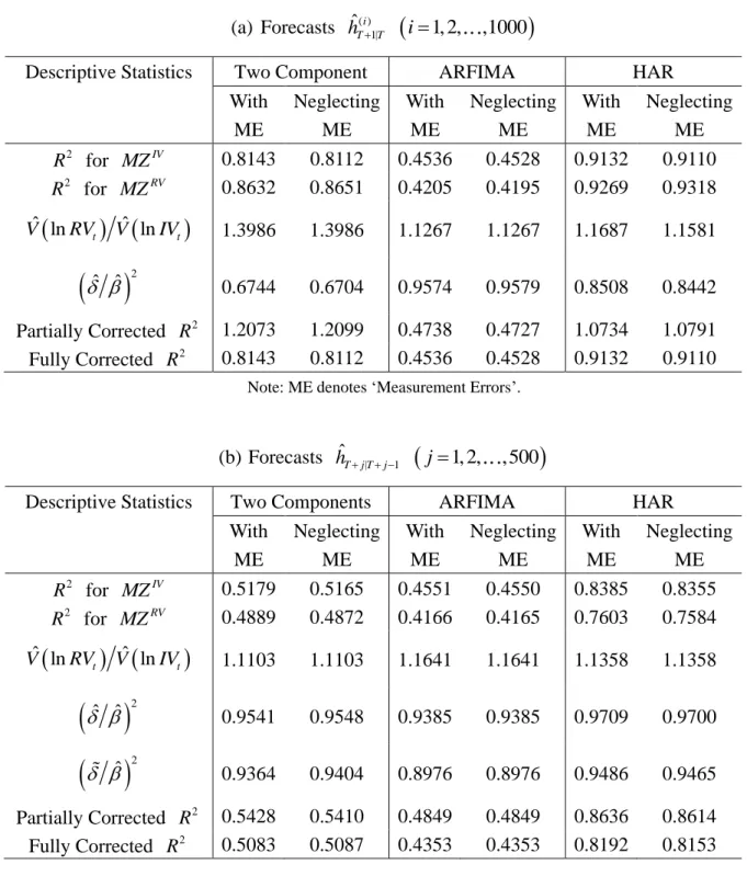
Regarding the previous Monte Carlo experiments, Table 5(a) shows the R2

based on MZRV and MZIV, and the partially corrected R2 by using the sample value of V



lnRV_t

 

V lnIV_t



. Clearly, the partially corrected R2 overestimates R2 for

IV

MZ , and it sometimes exceeds one, indicating that we have failed to use some important information.

The Appendix shows the algebraic relationship between R2 for MZRV and

IV

MZ , indicating that we need to multiply by not only the sample value of



ln _t

 

ln _t



V RV V IV but also by

 

2

ˆ ˆ

  . We will refer to this type of corrected R2

as the „fully corrected R2‟. Table 5 also presents the value of

 

 ˆ ˆ 2 and the fully corrected R2. This time the resulting R2 coincides with R2 for MZIV. Therefore, the full correction is needed for real data.

(18)

4.2 Proposed Approach



| 1 2 | 1 ˆ ˆ ˆ ˆ t t t t t h h w h h        



. (9)

The Appendix shows how to derive the connection between ˆ and ˆ . Equation (9) indicates that we also need to estimate w_t.

For this paper, we propose a simple method as follows. First of all, using the whole sample, including those for forecasting, we estimate the model taking account of the measurement errors. Second, for the estimated parameter value, we conduct filtering techniques below in order to obtain the filtered estimate of wt for the forecasting

period. Third, we obtain an estimate of ˆ by substituting the estimates of w_t for the true value of w_t in (9). Note that this estimate of w_t may be used not only for the model with measurement errors but also for the model neglecting measurement errors.

With respect to the filtering technique, we suggest the following approach. For the short-memory models including the ARMA and K-components models, we can use the Kalman filter. For the case of the long-memory ARFIMA model, we may use the filtering algorithm proposed by So (1999). Regarding nonlinear time series models, we can work with particle filters, such as in Kitagawa (1987). Note that another candidate for wt is the smoothed estimates.

(19)

For evaluating the forecasts of IV_t and IV_t2, a similar correction is required, in addition to the partial correction of Andersen, Bollerslev and Meddahi (2005) . The additional correction requires the estimation of w_t in RV_t IV_tw_t for volatility, and

2 2

t t t

RV IV w for volatility squared. If the models for log-volatility are considered, as in the current paper, we may use the particle filters for obtaining filtered estimates of

t

w , in general.

4.3 Simulation Results

In order to check the performance of the fully corrected approach, we conduct another Monte Carlo simulation. The previous Monte Carlo experiments considered the series of ˆ 1|

i T T

h _



i1, 2, ,500



. In other words, each ˆ 1|

i T T

h _ was calculated for the

i-th replication. Now we generate IV_t and RV_t with the same parameters and with the

sample size of T+500 once only. Then we forecast the model to obtain hˆ_T__{j T}_| _{ }_j ₁



j1, 2, ,500



, fixing the window size as T. For each forecast, the model is re-estimated. After forecasting, we estimate the model with the whole sample (T+500) in order to have the filtered estimate of w_t, w_t. On evaluating the forecasts using

RV

MZ , we can correct R2 by multiplying

 

2

ˆ

  for the corrected R2 by the sample value of V



lnRV_t

 

V lnIV_t



, where  is the estimate of ˆ based on (9) and w_t. It should be noted that the smoothed estimate of w_t is another proxy for w_t.

Table 5(b) shows the simulation results for R2 based on MZRV and MZIV, the partially corrected R2 by using the sample value of V



lnRV_t

 

V lnIV_t



, the

(20)

values of

 

2 ˆ ˆ   and

 

2 ˆ

  , and the fully corrected R2 based on

 

2

ˆ

  . We first analyse the results for the two component model. Roughly speaking, the difference between R2 for MZIV and the partially corrected R2 is 0.025, while the difference between the true R2 and fully corrected R2 is 0.01, such that the fully corrected R2

yields a better estimate of the true value. For the ARFIMA model, we have a similar result. The difference between R2 for MZIV and the partially corrected R2 is 0.03, while the difference between R2 for MZIV and fully corrected R2 is 0.02. With respect to the HAR model, the difference between R2 for MZIV and the partially corrected R2 is 0.025, while the difference between true R2 and fully corrected R2

is 0.02. In short, the fully corrected R2 can be far more accurate than its partially corrected counterpart in some cases, but it is never worse.

Before concluding the section, we discuss the effects of model misspecification. If the model is misspecified, which is typically the case for most models used in empirical research, the model misspecification error can be confused as a measurement error in finite samples. Hence, we need to separate the effect of measurement error from model misspecification error. For this purpose, we suggest using the most general model considered for the analysis in order to obtain the estimate of w_t. Note that the most general model need not produce the best out-of-sample forecasts, but it is expected to have best in-sample forecasts, that is, fitted values, if the sample size is large enough. In applied work, the true model may encompass the most general model considered for the analysis, yielding model misspecification error.

The fully corrected R2 is not worse in any case than its partially corrected counterpart, by construction. For the case of our simulation experiments, ARFIMA is the most general model, as the remaining two models have only ARMA representations. We obtained the filtered estimate of w_t, employing the ARFIMA model, for the case that each of the other two models is correct. Then we found that the results for the full corrected R2 remain unchanged.

(21)

5 Empirical Example

This section examines the estimates and forecasts using the RV of Standard and Poor‟s 500 Composite Index (S&P 500). In order to calculate the daily realized volatility, we use the estimation method given in ZMA (2005). The sample period is Jan/3/1996 to March/29/2007, giving T=2796 observations of RV.

We also compare the models given above with models including an MA(1) term, namely, the two component model (AR(1)+ARMA(1,1)), the ARFIMA(1,d,1) model, and the ARMA(22,1) with restrictions on the AR coefficients. The additional parameter is the coefficient of the MA(1) term, which is the same as the models with measurement errors. Intuitively, including the MA(1) term is more comprehensive than accommodating the measurement errors. We will use the first two models for estimating and forecasting IV. Instead of the last one, we consider the Heterogeneous ARMA (HARMA) model given by

5 22 1 1 2 1 3 1 1 1 5 22 1 1 2 3 1 1 1 1 ln ln ln ln 5 22 1 1 ln ln ln , 5 22 t t t i t i i i t t t i t i i i x  x  x  x                          



which is a natural extension of the HAR model.

Before estimating the models, it is useful to test for the existence of measurement errors. Tanaka (2002) proposed the LM statistic to test the presence of measurement errors based on three kinds of processes, namely the AR(p), unit root and long memory models. The test statistics have the standard normal distribution under the null hypothesis of no measurement error, and is one-sided on the right tail. Table 6 shows the test statistics for the logarithm of RV. When an AR(1) model is assumed to be the true process of the logarithm of IV, the calculated statistic rejects the null hypothesis of no measurement error. When an ARFIMA(1,d,0) process is assumed to be true, the calculated statistic also rejects the null hypothesis. The empirical results indicate that there are measurement errors which are not negligible, even after ostensibly removing

(22)

the microstructure noise.

Table 7 shows the QML estimates for the two-component model, accounting for and neglecting measurement errors. For the former, the estimated value of 1 is

close to 0.99, while the estimate of ₁ is 0.07, which are typical for SV models. For the second component, the estimate of ₂ is 0.80, while that of ₂ is 0.18. The

estimate of _w is 0.38, and is significant at the five percent level, indicating that measurement errors are not negligible. For the case of neglecting measurement errors, the estimates of ₁ and ₂ decrease, while those of ₁ and ₂ increase. As expected from the simulations, the differences for the second factor are large and not negligible, showing the large bias that are arise from neglecting the measurement errors. Table 7 also presents the QML estimates for the two component model comprising AR(1) and ARMA(1,1). The estimate of the MA(1) term is negative and significant. All other estimates, apart from 2, are close to those of QML with measurement errors.

Table 8 presents two kinds of QML estimates for the ARFIMA(1,d,0) model, one based on accommodating measurement error and another neglecting them. For the former, the estimate of d is 0.49, indicating that lnIV_t has long range persistence and is

stationary. The estimate of  is positive and significant, while the estimate of _w is close to that in Table 7. For the latter, the estimate of d is 0.48, for which the downward bias is expected from the simulations. The estimate of  is negative and significant. Table 8 also gives the estimates of ARFIMA(1,d,1) as a counterpart to the ARFIMA(1,d,0) model accommodating measurement error. The estimate of the MA term is positive and significant.

Table 9 presents estimates for the HAR model. For case accounting measurement errors, the estimate of  ₁ ₂₃ is 0.96, which implies high

(23)

persistence in volatility. The estimate of _w is 0.33, which is smaller than those in Tables 7 and 8. Regarding the case neglecting measurement error, the estimate of

1 2 3

   is 0.93, but the estimates of each parameter is different from those of the former. We also estimated the HARMA model, which is the ARMA(22,22) with restrictions on the AR and MA coefficients. The estimate of the MA term is negative and significant. The estimate of  ₁ ₂₃ is 0.98, while   ₁ ₂ ₃ is 0.648. The estimates of ₁ and ₃ are significant, while that of ₂ is insignificant.

Next, we compare the out-of-sample forecasts based on these three approaches. The period of forecast is the last 796 observations. For each set of forecasts, the parameters are re-estimated to calculate the forecasts, fixing the sample size to 2000.

The forecasts are evaluated by estimating the Mincer-Zarnowitz regression,

RV

MZ . We compute the partially corrected R2 values, as proposed in Andersen, Bollerslev and Meddahi (2005), as a measure of the ability of the model to track the variance over time. We also calculate the fully corrected R2 values, as proposed in the previous section, but do not calculate the mean absolute errors or root mean squared errors as they neglect the measurement error in realized volatility.

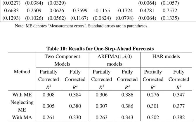
Table 10 reports the partially and fully corrected R2 values for the two-component, ARFIMA(1,d,0) and HAR models. For estimating w_t with the full correction, we use the ARFIMA model, as discussed in the previous section. The differences between the partially and fully corrected R2 values are not negligible, implying the importance of taking account of the measurement error fully in correcting

2

R . The partially corrected R2 selects the two component model accommodating the measurement error, while the fully corrected R2 chooses the ARFIMA models with/without measurement error. This can happen as in the Monte Carlo simulations, which suggest that the fully corrected R2 provides a more accurate estimate of the true

2

(24)

corrected R2 values show that the ARFIMA models with/without measurement errors have the highest value, while the two-component model with the MA(1) term has the lowest. We will examine the differences among the models with and without measurement errors. As stated previously, the ARFIMA models have the highest value of the fully corrected R2, while the HAR model with measurement error has the lowest. The second best model is the two-component model with measurement error, while the remaining two models have similar values.

has an interpretation that

2t

f contains useful information that is not present in f₁_t. For the case 0, f₁_t is said to “encompass” f₂_t.

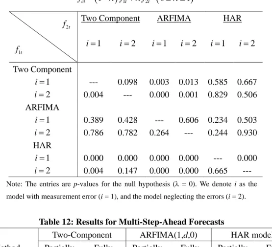
Table 11 gives the p-values of the test of Harvey, Leybourne and Newbold (1998) with respect to the models with/without measurement errors. The forecasts of both ARFIMA models encompass all the other forecasts. The forecast of the two factor model with measurement error encompasses the remaining three models. The forecast of the HAR model with measurement error encompasses no forecasts. The implication obviously supports the fully corrected R2 values in Table 10. Note that the test of forecast encompassing is not suitable for model evaluation for the following two reasons: (i) it neglects the measurement errors, and (ii) the test may potentially find two forecasts which are unable to encompass each other.

Table 12 gives the partially and fully corrected R2 values for the h step-ahead forecasts (h=5, 10, 20), regarding the two component, ARFIMA and HAR models with/without measurement errors and with the MA term. The differences between the partially and fully corrected R2 values are not negligible. In all cases, the fully

(25)

corrected R2 chooses the HAR model with measurement errors. For the cases h=5 and 10, the two component (AR(1)+ARMA(1,1)) model has the lowest values of the fully corrected R2, whereas for the case h=20, the ARFIMA model neglecting measurement errors is chosen.

6 Conclusions

Neglecting microstructure noise in calculating RV can lead to inconsistent estimates of the IV as a true measure of volatility. Consequently, several methods have recently been proposed to remove the effects of microstructure noise and to obtain consistent estimates of the IV. However, even bias-corrected and consistent RV estimates of the IV contain RV errors that should not be ignored.

This paper investigated the effects of RV errors on estimating and forecasting models of IV. For minor RV errors, the Monte Carlo results showed that: (i) the estimates neglecting measurement error have serious biases; (ii) forecasts accounting for the measurement error outperform those neglecting them, but the differences can be small; and (iii) R2 for evaluating the forecasts should be corrected appropriately.

This paper also proposed a new method to correct R2 of the Mincer-Zarnowitz regression, which is based on measurement. Monte Carlo results showed that the new fully corrected method is preferred to the partially corrected approach of Andersen, Bollerslev and Meddahi (2005).

The empirical example of S&P 500 showed that neglecting microstructure noise can cause serious bias in estimating IV. Such bias in forecasting was found to be small. The proposed fully corrected R2 showed the clear difference with the partially corrected R2 of Andersen, Bollerslev and Meddahi (2005).

(26)

Data

Appendix: Construction of Daily Realized Volatility Measures

The empirical analysis focuses on the RV of the S&P 500 index. We start by removing non-standard quotes (discarding quotes where the bid or offer price is missing and selecting observations where the “mode” field in the TAQ file is 3, 5, 10, 12 or 29), computing prices through the mean of the bid and ask quotes, filtering possible errors, and obtaining one second returns for the 9:30 am to 4:00 p.m. period.

Observing the consistency considerations in Hansen and Lunde (2006), the previous tick method for determining prices at precise second marks is implemented. In order to calculate the daily RV, we use the estimation method given in BHLS (2008).

Appendix: Fully Corrected

2

R

Consider the following structure of noise

t t t

y  x w , (A.1)

where x_t follows a dependent process, and w_t is correlated with x_t. Although x_t is

assumed to be latent, we can observe yt. We denote the forecast of xt as ˆht, where

t

y and x_t in (A.1) correspond to lnRV_t and lnIV_t , respectively. Regarding the two Mincer-Zarnowitz regressions:

ˆ _error, ˆ _error. t t t t x h y h           (A.2) 2 R is given as

 





2 2 2 2 ˆ ˆ ˆ t x t h h R x x    



, and



 



2 2 2 2 ˆ ˆ ˆ t y t h h R y y    

2 ˆ ˆ   . Hence,

 

2 ˆ ˆ ˆ ˆ ˆ ˆ t t t h h w h h     



, (A.3)

in which the second term in (A.3) does not approach zero as T   because of the correlation between ˆh_t and wt. Multiplication of

2

y

R by



Andersen, T.G.. and T. Bollerslev (1998), “Answering the skeptics: Yes, standard volatility models do provide accurate forecasts”, International Economic Review, 39, 885 – 905.

Andersen, T., T. Bollerslev, F.X. Diebold and H. Ebens (2001), “The distribution of realized stock return volatility”, Journal of Financial Economics, 61, 43–76.

Andersen, T.G., T. Bollerslev, F.X. Diebold and P. Labys (2003), “Modeling and forecasting realized volatility”, Econometrica, 71, 529 – 626.

Andersen, T., T. Bollerslev and N. Meddahi (2005), “Correcting the errors: A note on volatility forecast evaluation based on high-frequency data and realized volatilities,” Econometrica, 73, 279 – 296.

Asai, M. (2008), “Autoregressive stochastic volatility models with heavy-tailed distribution: A comparison with multifactor volatility models”, Journal of Empirical Finance, 15, 332-341. Asai, M., M. McAleer and J. Yu (2006), “Multivariate stochastic volatility: A review”,

Econometric Reviews, 25, 145 – 175.

Bandi, F.M. and J.R. Russell (2007), “Volatility estimation”, In J. Birge and V. Linetsky eds.,

Handbook in Operations Research and Management Science: Financial Engineering, North Holland, Elsevier, 183－222.

Barndorff-Nielsen, O.E., and N. Shephard (2002), “Econometric analysis of realized volatility and its use in estimating stochastic volatility models”, Journal of the Royal Statistical Society,

Series B, 64, 253－280.

Barndorff-Nielsen, O.E., P.H. Hansen, A. Lunde and N. Shephard (2008), “Designing realised kernels to measure the ex-post variation of equity prices in the presence of noise”,

Econometrica, 76, 1481－1536.

Bollerslev, T. (1986), “Generalized autoregressive conditional heteroskedasticity”, Journal of Econometrics, 21, 307 – 328.

Breidt, F.J., N. Crato and P.J.F. de Lima (1998), “The detection and estimation of long-memory in stochastic volatility”, Journal of Econometrics, 83, 325 – 348.

Chernov, M., A.R. Gallant, E. Ghysels and G. Tauchen (2003), “Alternative models for stock price dynamics”, Journal of Econometrics, 116, 225 – 257.

Corradi, V. and W. Distaso (2006), “Semiparametric comparison of stochastic volatility models using realized measures”, Review of Economic Studies, 73, 635－677.

Corsi, F. (2009), “A simple approximate long memory model of realized volatility,” Journal of Financial Econometrics, 7, 174-196.

(29)

Engle, R.F. (1982), “Autoregressive conditional heteroskedasticity with estimates of the variance of United Kingdom inflation”, Econometrica, 50, 987－1007.

Ghysels, E., A.C. Harvey and E. Renault (1996), “Stochastic volatility”, In C. R.Rao and G. S. Maddala eds., Statistical Methods in Finance, pp.119－191. Amsterdam: North-Holland. Hansen, P.R., J. Large and A. Lunde (2008), “Moving average-based estimators of integrated variance”, Econometric Reviews, 27, 79－111.

Hansen, P.R. and A. Lunde (2006), “Realized variance and market microstructure noise” (with discussion), Journal of Business and Economic Statistics, 24, 127 – 218.

Harvey, A.C. (1998), “Long memory in stochastic volatility”, in J. Knight and E. Satchell (eds.),

Forecasting Volatility in Financial Markets, Butterworth–Haineman, London, pp. 307–320. Harvey, A. C. and N. Shephard (1996), “Estimation of an asymmetric stochastic volatility model for asset returns”, Journal of Business and Economic Statistics, 14, 429-34.

Kitagawa, G. (1987), “Non-Gaussian state-space modeling of nonstationary time series,”

Journal of the American Statistical Association, 82, 1032－1063 (with discussion).

McAleer, M. (2005), “Automated inference and learning in modeling financial volatility”,

Econometric Theory, 21, 232 – 261.

McAleer, M. and M. Medeiros (2008a), “Realized volatility: A review”, Econometric Reviews, 27, 10－45.

Meddahi, N. (2002), “A theoretical comparison between integrated and realized volatility”,

Journal of Applied Econometrics, 17, 479 – 508.

Nelson, D. B. (1990), “ARCH models as diffusion approximations”, Journal of Econometrics,

45, 7–38.

Nelson, D. B. (1991), “Conditional Heteroskedasticity in Asset Returns: A New Approach”,

Econometrica, 59, 347－70.

So, M.K.P. (1999), “Time series with additive noise”, Biometrika, 86, 474－482.

Tanaka, K. (2002), “A unified approach to the measurement error problem in time series models”, Econometric Theory, 18, 278 – 296.

Taylor, S.J. (1986), Modelling Financial Time Series, Wiley, Chichester.

Zhang, L., P.A. Mykland and Y. Aït-Sahalia (2005), “A tale of two time scales: Determining integrated volatility with noisy high frequency data”, Journal of the American Statistical Association, 100, 1394 – 1411.

(30)

Table 1: Results of the QML Estimators for the Two-Component Model for T=1000

(a) Finite Sample Properties

Parameter True With Measurement Errors Neglecting Measurement Errors

Value Mean St.Dev. RMSE Mean St.Dev. RMSE

1  0.98 0.9701 0.0137 0.0169 0.9663 0.0158 0.0210 1  0.10 0.1040 0.0213 0.0217 0.1131 0.0230 0.0265 2  0.40 0.4044 0.1055 0.1055 0.2939 0.0546 0.1193 2  0.40 0.4164 0.0586 0.0609 0.4750 0.0284 0.0802  1.00 1.1452 0.1471 0.2067 1.1457 0.1470 0.2069 w  0.1745 01759 0.1287 0.1287

Note: The true value of _w is obtained by simulation.

(b) One-Step-Ahead Predictions

Statistic With Measurement Errors Neglecting Measurement Errors

1,T 1

 _ 2,T1 lnIVT1 1,T1 2,T1 lnIVT1

MAE 0.2325 0.2790 0.2294 0.2337 0.2839 0.2307

RMSE 0.2910 0.3512 0.2968 0.2952 0.3568 0.2987

(c) Mincer-Zarnowitz Regression

Method With Measurement Errors Neglecting Measurement Errors

2 R F test 2 R F test IV MZ 0.8143 0.0000* 0.8112 0.0000* RV MZ 0.8632 0.0000* 0.8651 0.0000*

Note: „F test‟ denotes the p-value of the (robust) 2 test for the null hypothesis of

0 and 1

(31)

Table 2: Results of the QML Estimators for the ARFIMA Model for T=1000

d 0.40 0.4099 0.0664 0.0671 0.3755 0.0410 0.0477   0.40 0.3756 0.0758 0.0797 0.4411 0.0235 0.0474  -0.10 -0.0444 0.1581 0.1676 -0.1051 0.0473 0.0476 w  0.1537 0.1515 0.1369 0.1369

(b) One-Step-Ahead Predictions of lnIV_T_₁

MAE 0.3154 0.3158

RMSE 0.3919 0.3922

2 R F test 2 R F test IV MZ 0.4536 0.5918 0.4528 0.5969 RV MZ 0.4205 0.3915 0.4195 0.7808

Note: „F test‟ denotes P-value of the (robust) 2 test for the null hypothesis of

0 and 1

(32)

Table 3: Results of the QML Estimators for the ARFIMA Model for T=2000

d 0.40 0.4116 0.0465 0.0479 0.3766 0.0277 0.0362   0.40 0.3800 0.0673 0.0702 0.4393 0.0189 0.0436  -0.10 -0.0564 0.1211 0.1287 -0.1037 0.0338 0.0340 w  0.1537 0.1484 0.1284 0.1285

MAE 0.3157 0.3158

RMSE 0.3947 0.3949

2 R F test 2 R F test IV MZ 0.3967 0.0885 0.3959 0.1148 RV MZ 0.3639 0.3191 0.3628 0.3549

0 and 1

(33)

Table 4: Results of the Estimators for the HAR Model for T=1000

1  0.80 0.7915 0.1337 0.1339 0.4448 0.0840 0.3650 2  0.10 0.0995 0.1252 0.1252 0.3878 0.0844 0.2999 3  0.05 0.0478 0.0331 0.0332 0.0724 0.0473 0.0524   _0.25 _{0.2629 0.0503 0.0520 0.4016} _0.0458 _0.1583  1.00 0.9913 0.1508 0.1511 0.9895 0.1558 0.1561 w  0.2637 0.2445 0.0655 0.0683

MAE 0.1432 0.1440

RMSE 0.1841 0.1871

2 R F test 2 R F test IV MZ 0.9132 0.0000* 0.9107 0.0000* RV MZ 0.9269 0.0000* 0.9318 0.0000*

0 and 1