Improving GARCH Volatility Forecasts
by Franc Klaassen
∗Department of Econometrics, Tilburg University
May 13, 1998
Abstract
Many researchers use GARCH models to generate volatility forecasts. We show, however, that such forecasts are too variable. To correct for this, we extend the GARCH model by distinguishing two regimes with different volatility levels. GARCH effects are allowed within each regime, so that our model generalizes existing regime-switching models that allow for ARCH terms only. The empirical application on U.S. dollar exchange rates shows that our model indeed yields better volatility forecasts than single-regime GARCH and that the allowance for GARCH terms besides ARCH terms can be crucial for the forecast quality.
Key words:
GARCH, regime-switching, volatility, forecasting, exchange rates.JEL classification:
C52, C53, F31.∗Correspondence to: Franc Klaassen, Department of Econometrics, Tilburg University, P.O.
Box 90153, 5000 LE Tilburg, the Netherlands; tel: +31-13-4668229; fax: +31-13-4663280; E-mail: [email protected].
I would like to thank Frank de Jong, Harry Huizinga, Theo Nijman, Casper de Vries and Bertrand Melenberg, as well as Arthur van Soest and Geert Bekaert for their helpful comments.
1
Introduction
Exchange rates play a key role in the international economy. There is a lot of currency trading on financial markets, and also in international goods trade at least one of the trading partners has to deal with a foreign currency. Not only the levels of exchange rates are important, also their volatility is. For example, exchange rate volatility is important in the pricing of currency options and may also affect international trade.
It is well-known that volatility is time-varying in high-frequency data and that periods of high volatility tend to cluster. To capture this, many authors have used autoregressive conditional heteroskedasticity (ARCH) models, as introduced by
En-gle (1982) and extended to generalized ARCH (GARCH) in Bollerslev (1986).1 Such
models usually improve the fit a lot compared with a constant variance model and, as Andersen and Bollerslev (1997) claimed, GARCH models provide good volatility forecasts.
In this paper we show that GARCH forecasts are, nevertheless, too variable. We try to improve on the GARCH forecasts by extending the GARCH model such that this weakness disappears. Therefore, our model contains an extra source of volatility per-sistence by distinguishing two regimes with different volatility levels. GARCH formulas are used to capture any volatility persistence within the regimes. The resulting regime-switching GARCH model indeed yields better volatility forecasts, both one-period and multi-period-ahead, in-sample as well as out-of-sample.
What is the reason behind the high variability of standard GARCH volatility fore-casts? It is well-known that GARCH models often imply a high volatility persistence of individual shocks. For example, for their stock return data Hamilton and Susmel (1994) showed that a shock this week will have a nonnegligible effect on the variance a full year later. Therefore, GARCH models are unable to capture the fact that shocks sometimes have the effect of ”relieving pressure” on the system, that is, a shock is followed by a period of low instead of high volatility. The source of volatility persis-tence that we add to standard GARCH models makes that individual shocks can, but need not be persistent. Our empirical results make clear that this greater flexibility in the persistence of shocks removes the too high a variability of the volatility forecasts. Apparently, it is the high volatility persistence that makes standard GARCH forecasts too variable.
Lamoureux and Lastrapes (1990), among others, showed that the high volatility persistence in GARCH models may originate from structural changes in the variance
1
process. They demonstrated that any shift in the unconditional variance is likely to lead to misestimation of the GARCH parameters in such a way that they imply too high a volatility persistence. For example, if the variance is high but constant for some time and low but constant otherwise, persistence of such high and low homoskedas-tic periods already results in volatility persistence. A GARCH model, which cannot capture persistence of such periods, puts all volatility persistence in the persistence of individual shocks.
Structural changes in the variance process can originate from changes in economic policy, such as the change in U.S. monetary policy in 1979, when the Federal Reserve reduced the money growth rate to bring down inflation and to stop the dollar’s fall. Sudden shifts may also result from more exogenous changes in the economic environ-ment, such as the OPEC oil crises.
One possibility to allow for periods with different unconditional variances is, of course, by introducing deterministic shifts into the variance process, but this is rather ad hoc. A popular approach to endogenize changes in the data generating process is the use of a Markov regime-switching model. Hamilton (1989) introduced this model to describe the U.S. business cycle, which is characterized by periodic shifts from recessions to booms and vice versa. In our context of exchange rate volatility, a Markov process can be used to govern the switches between regimes with different variances. Even a simple regime-switching model with constant regime-specific variances already captures a lot of the volatility persistence, as our empirical results show.
To capture the remaining conditional heteroskedasticity, the Markov approach can be combined with ARCH models, as Cai (1994) and Hamilton and Susmel (1994) showed. Their regime-switching ARCH models have two ways to capture volatility persistence, namely the persistence of regimes and the ARCH effects within a regime. We show empirically that for some series a moderate number of ARCH terms is indeed sufficient to capture all conditional heteroskedasticity.
A potential drawback of regime-switching ARCH models is that only ARCH models are allowed within a regime, not GARCH models. Our empirical results show that this is not only a theoretical disadvantage, but that it is also important from a practical point of view, as some series are characterized by long persistence of shocks within a regime. One GARCH term can capture such long persistence much more parsimoniously than a large number of ARCH terms. Moreover, as we show, neglecting the long persistence can result in even worse volatility forecasts than those generated by a single-regime GARCH model. For that reason Gray (1996a) modified the approaches of Cai (1994) and Hamilton and Susmel (1994) such that also GARCH effects are allowed in each
variance regime.
Our variance specification also allows for GARCH effects. The crucial difference with Gray’s model is the way the unobserved regime indicator is integrated out. We use all available information, whereas Gray uses only part of it. The important result of this is that we get much simpler, first-order recursive variance forecasting formulas. Together with the first-order recursive structure of the likelihood function, this makes the model very useful from a practical point of view.
Another feature of our model is that volatility persistence of individual shocks is allowed to be different across regimes. Our empirical results show that in periods of high volatility shocks are more persistent than in low volatility periods. Cai (1994) and Hamilton and Susmel (1994) did not account for this, but Gray (1996a) did. A shift from the high variance to the low variance regime is thus only part of the way to explain the ”pressure relieving” effect discussed above. The other part results from the fact that the regime shift also implies a shift to the low-persistence regime. Besides the introduction of two variance regimes, this leads to additional flexibility regarding the persistence of shocks. Recall that it is the spuriously high persistence in single-regime GARCH models that causes the high variability of the forecasts.
In the next section we will formally introduce our regime-switching GARCH model. The recursive estimation process is described in section 3, after which section 4 describes alternative ways to determine the regime the process was likely in at a particular time. Section 5 presents the recursive forecasting formula that makes volatility forecasting in our regime-switching GARCH model much easier than in Gray’s (1996a) model. In section 6 we describe the twenty years of daily U.S. dollar exchange rates vis-a-vis the British pound, the German mark and the Japanese yen that we use in our empirical application. The empirical results are also in this section. Finally, section 7 concludes.
2
Regime-Switching GARCH Model
In this section we present regime-switching models to capture the conditional het-eroskedasticity that is present in many high-frequency financial time-series. We first discuss regime-switching models in the literature so far, and then, having showed the problems involved in them, we introduce our regime-switching GARCH model.
LetStdenote the logarithm of a spot exchange rate at timet. Since there is
substan-tial empirical evidence that exchange rates themselves are not covariance stationary, but that their first differences are (see Hakkio and Rush (1989)), we analyze the return
st= 100(St−St−1). Thus, st is the percentage depreciation from time t−1 to time t.
As the paper is mainly focussed on modeling return volatility rather than its level,
we assume for simplicity that theconditional meanof st is constant:
st=µ+εt, (1)
where the error term εt satisfiesEt−1{εt}=E{εt|It−1}= 0.2 Thus,µ=Et−1{st}is the
expected depreciation.
To model theconditional varianceofstmany authors have used GARCH models.
This improves the fit a lot, and the implied persistence of individual shocks in the variance is usually very high (see Hamilton and Susmel (1994)). This high volatility persistence may be spurious and originate from instability of the GARCH parameters, as Lamoureux and Lastrapes (1990) demonstrated. As argued in the introduction, we take account of this instability by the introduction of two variance regimes as a second source of volatility persistence. Let rt be the (unobserved) regime at timet−1,
where the first regime is identified as the low variance one. We will now discuss four specifications for Vt−1{εt|rt}, the variance conditional on observed information It−1
and on the unobserved regime being rt.
One possible specification for the conditional variance is a GARCH(1,1) model. In a regime-switching context, this would define
Vt−1{εt|rt}=ωrt+αrtε 2
t−1+βrtVt−2{εt−1|rt−1}, (2)
where the current regime only determines the parameters, that is, the intercept ωrt,
the ARCH parameter αrt and the GARCH parameter βrt. However, the previous
conditional variance Vt−2{εt−1 |rt−1} cannot be computed, since we do not observe
regimes. Moreover, Vt−2{εt−1|rt−1} depends on Vt−3{εt−2|rt−2}, which depends on
Vt−4{εt−3 |rt−3}, and so on. Consequently, the conditional variance in (2) depends
on the entire sequence of variance regimes up to time t. Each different combination
of previous regimes thus leads to a different conditional variance at time t. Since the
number of possible combinations grows exponentially witht, this leads to an enormous
number of regime paths to t. This renders estimation intractable, since the likelihood
contribution of observationt is constructed by integrating out over all possible regime
paths.
In the literature so far we find two different approaches to circumvent this problem of path dependence. First, Cai (1994) and Hamilton and Susmel (1994) essentially removed the GARCH term, which is the cause of the path dependence, from (2) and
2It is possible to incorporate, for example, autoregressive terms in the conditional mean without
thus used only ARCH terms.3 Therefore,V
t−1{εt|rt}in (2) only depends on the current
regimert.4
However, as Gray (1996a) argued, the problem of path dependence can be solved without giving up the potentially important persistence effects of a GARCH term. Gray first integrated out the unobserved regime rt−1 in Vt−2{εt−1|rt−1} in (2) using
the information observable at time t−2 and then used the aggregated variance in a
GARCH formula:
Vt−1{εt|rt}=ωrt +αrtε 2
t−1+βrtEt−2{Vt−2{εt−1|rt−1}}. (3)
By integrating out the regimert−1he obtained a conditional variance that only depends
on the current variance regimert, not on previous regimes. He thus avoided the problem
of path dependence by a slight redefinition of the GARCH(1,1) formula in (2). He showed that the likelihood function can be computed recursively, similar to that in a single-regime GARCH model.
There is one important problem with Gray’s method: generating variance forecasts
Vt−1{st−1+l}for some leadl >1 turns out to be very complicated. The approach we will
use does not have this problem with forecasting. Furthermore, our approach also allows for persistence effects through a GARCH term, without suffering from the problem of path dependence.
The improvement of our model with respect to forecasting is due to two crucial differences with Gray’s model. First, as the expectation in (3) shows, Gray integrated out the regimert−1 at timet−2. We postpone this tillt−1, the time at which we want
to compute the conditional variance. This allows us to use more observable information when integrating out the previous regime. The extra data embodies information about previous regimes and is thus useful.
The second crucial difference is that, when integrating out the regime rt−1, Gray
did not use the information that the variance regime at time t is in the conditioning
information of Vt−1{εt|rt}. Particularly if regimes are highly persistent, the variance
regime at time t will give much information about the regime at t−1. In contrast to
Gray, we do use that information.
3In both papers the authors use more than one lag in the ARCH specification. All results in the
present paper can be generalized to include also more than one lag in a straightforward manner. It is only for the sake of exposition that we restrict the number of lags to one.
4Cai (1994) and Hamilton and Susmel (1994) used slightly different models in whichV
t−1{εt|rt}
not only depends on the current but also on a few recent regimes. The essential point is that the conditional variance depends on a small number of regimes, so that the short regime paths can be integrated out quite easy.
In formula, our regime-switching GARCH(1,1) model is described by
Vt−1{εt|rt}=ωrt +αrtε 2
t−1+βrtEt−1{Vt−2{εt−1|rt−1}|rt}. (4)
Thus, we take the mean of (2) over the previous regimert−1 conditional on all available
information, that is, the observable information at timet−1,It−1, and the information
about the current variance regime rt. By construction,Vt−1{εt|rt} only depends on
the current variance regime rt, so there is no path dependence. In section 5 we shall
show that this approach indeed leads to relatively simple, recursive formulas for the conditional variance Vt−1{st−1+l} of future exchange rate returns.
To ensure positivity of Vt−1{εt|rt} for all t, we assume ωrt > 0 and αrt, βrt≥0.
We also assume that the ”unconditional” varianceV{εt|rt}exists for both regimes for
all ω1 and ω2. Necessary conditions for this are in appendix A, which also provides
a formula for the unconditional variance. The necessary conditions are similar to the
necessary (and sufficient) condition α+β<1 in the one-regime GARCH(1,1) model.
It is clear from above that, even within a regime, we allow for volatility persis-tence. The exact nature of this persistence is allowed to differ between regimes. For instance, if shocks are more persistent in periods of high volatility than in periods of low volatility, the regime specific parameters in (4) are able to capture this asymmetry. This has important consequences for capturing the ”pressure relieving” effect of some large shocks. That is, sometimes a shock relieves the market from tensions, so that the period following the shock is quiet rather than volatile. Any regime-switching model can capture this to some extent by a shift from the high volatility to the low volatility regime. However, our regime-switching model with different parameters across regimes has an additional source of neglecting large recent shocks. If the low variance regime is the short persistence regime, the large shock will be out of the market very soon after the switch to the low variance regime. This extra flexibility regarding the volatility persistence of shocks will prove important in the empirical analysis. In this respec-t, our model generalizes the models in Hamilton and Susmel (1994) and Cai (1994), even if GARCH terms are not present. After all, their regime variances only differ by a multiplicative or additive constant, respectively, not by differences in the ARCH parameters.
Given our specification of the conditional mean and variance, the regime-specific
conditional return distribution is completed by the assumption that, conditional
on the observable information It−1 and on the regime being rt, the error term has a
t-distribution withνrt degrees of freedom, zero mean and varianceVt−1{εt|rt}:
We choose a t-distribution instead of a normal one to allow for leptokurtosis even in the regime-specific conditional distribution. We will show empirically that this is particularly important in regime-switching models, since it improves the stability of the regimes. In case of normality, a large innovation in the low volatility period will lead to a switch to the high volatility regime earlier, even if it is a single outlier in an otherwise quiet period. Note that the t-distribution includes the normal distribution as a limiting case as the degrees of freedom go to infinity.
So far, we have described the exchange rate return process conditional on the regime.
To complete the model, we now describe theregime process. As in Hamilton (1989),
we assume that the latent variance regime indicator rt follows a Markov process with
constant staying probabilities
pt−1(rt|rt−1) =p(rt|rt−1) = p11 ifrt=rt−1= 1 p22 ifrt=rt−1= 2. (6)
Thus, the conditional probability that the current regime is the low or high variance
regime depends on the past only through the most recent regime rt−1. Both staying
probabilities are strictly between zero and one, so that there is no absorbing regime. Equations (1), (4), (5) and (6) describe the complete regime-switching GARCH
model. The first three equations determine the density of the exchange rate st
con-ditional on It−1 and on the variance regime rt, as we will show in the next section.
The last equation describes the regime process, which will be needed to integrate out the unobserved regimes. Note that the standard, one-regime GARCH(1,1) model is a special case of our model, with, of course, the regime process left out.
3
Estimation
We estimate the regime-switching GARCH model by maximum likelihood. To obtain
the likelihood function, we first need the density of the exchange rate return at time t
conditional on only observable information. Let pt−1(st) denote this density evaluated
at an exchange rate return equal to st. We have
pt−1(st) =
X
rt=1,2
pt−1(st|rt)·pt−1(rt). (7)
The first term on the right-hand-side,pt−1(st|rt), denotes the density of the exchange
rate return at time t evaluated at the value st conditional on It−1 and on the regime
having valuert. This density follows from equations (1), (4) and (5). These imply that,
have the following t-distribution: st|It−1, rt ∼ t(νrt , µ , Vt−1{εt|rt}) , (8) where Vt−1{εt|rt}=ωrt +αrt(st−1−µ) 2+β rtEt−1{Vt−2{εt−1|rt−1}|rt}. (9)
Since the regime in the conditioning information in (8) is unobservable, it has to be integrated out using the second term in (7),pt−1(rt), which is the conditional probability
that the variance regime at t has value rt. This makes the density of st conditional
on only observable information a mixture of two t-distributions, with a time-varying mixing parameter. Appendix B presents a simple formula to compute pt−1(rt). It also
gives a simple formula for the probabilitypt−1(rt−1|rt), which is needed to compute the
expectation in (9). Furthermore, both probabilities and all other regime probabilities in the paper can be derived from only one key probability, which is pt−1(rt−1). Using
similar techniques as in Gray (1996a), we show in appendix B that this key probability has a first-order recursive structure, which simplifies its computation a lot.
Summarizing the computation of the densitypt−1(st), we have shown that one only
needs the first-order recursive key probability for the two regime outcomes, the previous returnst−1 and two previous variancesVt−2{εt−1|rt−1}. Therefore, computingpt−1(st)
for allt is a first-order recursive process, similar to that of a one-regime GARCH(1,1)
model. This is a very important implication of the path independent modeling of the conditional error variance in (4). Integrating out the previous regime at each recursion implies that one can forget about earlier regimes, and this makes the calculation of the densities quite fast.
These densities can now be used to build the sample log-likelihoodPTt=1log(pt−1(st))
with which all parameters in the regime-switching GARCH model can be estimated. To start up the recursive computation of the log-likelihood, we set the required variables equal to their expectation without conditioning on the information set. In appendix A we derive the ”unconditional” varianceV{εt|rt}, which is used to start-upVt−1{εt|rt}
att= 1.
4
Regime Inference
An interesting aspect of regime-switching models is that one can endogenously de-termine when the variable under consideration was likely in the high or low variance regime. The regime probabilities used so far, such as pt−1(rt) and pt−1(rt−1), use only
probability, while pt−1(rt−1) is a filter probability (see Gray (1996a)). However, if one
is interested in determining ex post when the process was likely in a particular regime
at timet, one can use all information there is at the timeτ ≥tone wants to compute
the probability. Let pτ(rt) denote the ex post probability.
An ex post regime probability that is of special interest is the smoothed probability
pT(rt), which uses all information in the dataset (τ=T). It gives the most efficient
answer to the question which regime the process was likely in at time t. Smoothed
regime probabilities have been used in many papers for such regime inference (see Gray (1996a) and Cai (1994)).
In appendix C we show that all ex post regime probabilitiespτ(rt) can be computed
recursively. The algorithm is based on Gray (1996b). It links the ex ante probabilities, which are used during estimation, directly to the ex post probabilities by iterating
forward from the ex ante to the ex post probabilities. Note that forτ=tthis algorithm
gives the filter probabilities.
5
Forecasting
One of the advantages of our regime-switching GARCH model over Gray’s (1996a) model is the ease of multi-period-ahead forecasting. Suppose one is interested in the variance of thel-period-ahead exchange rate returnst−1+lgiven information available at
timet−1. For notational convenience, letτ denote the future time, that is,τ=t−1+l ≥t. The variance of interest is
Vt−1{sτ}=
X
rτ=1,2
pt−1(rτ)·Vt−1{ετ|rτ}. (10)
An important implication of our way of modeling the conditional variance in (4) is
that Vt−1{ετ|rτ} can be computed in a recursive manner using a formula analogous
to the one Engle and Bollerslev (1986) derived for the standard, one-regime GARCH model. Starting from Vt−1{εt|rt}, which is a by-product of the calculation of the
density pt−1(st), one can compute Vt−1{ετ|rτ}forτ > t by iterating forward on
Vt−1{εt+i|rt+i}=ωrt+i + (αrt+i+βrt+i)·Et−1{Vt−1{εt+i−1|rt+i−1}|rt+i},
(11) fori= 1, ..., τ−t. This recursive formula is proved in appendix D. 5 It makes the com-putation of Vt−1{sτ} in (10) quite easy. These multi-period-ahead volatility forecasts
will be compared to the standard, one-regime GARCH(1,1) forecasts in the empirical application of the next section.
6
Empirical Results
In this section we examine empirically the quality of the regime-switching GARCH model developed in section 2. First, we describe the data. Then we estimate the model and analyze the differences between the regime-switching GARCH model and the standard, single-regime GARCH(1,1) model. We also compare our regime-switching GARCH model with regime-switching ARCH models similar to the ones used by Cai (1994) and Hamilton and Susmel (1994), so that we can examine whether the GARCH effects, which they neglect, are practically relevant. Finally, we examine whether the introduction of the regime-switches to the GARCH model has indeed resulted in better volatility forecasts.
6.1
Data
We use three major U.S. dollar exchange rates, namely, the dollar vis-a-vis the British
pound, the German mark and the Japanese yen.6 We have 4982 daily observations for
the exchange rate returnstfrom January 3, 1978 to July 23, 1997. All rates have been
obtained from Datastream.
Panel A of figures 1, 2 and 3 at the end of section 6.2 gives an indication of the volatility clustering of the three exchange rates under consideration over the sample
period. We present the squared returns, s2t, instead of the returns themselves to get
a clearer distinction between periods of high and low volatility. This is also useful when assessing the quality of the volatility forecasts, which will be done below. All three squared return plots show substantial volatility clustering, indicating the potential usefulness of allowing for conditional heteroskedasticity.
The plots also demonstrate that shocks sometimes have a long effect on subsequent volatility, but that shocks can also be followed by a period of low volatility. To show whether single-regime GARCH, regime-switching ARCH and regime-switching GARCH models can capture this, let us consider figure 1A as an example. The large peak in the squared return plot for the British pound on March 27, 1985 was followed by about half a year of substantial volatility. Single and multi-regime ARCH models cannot capture such long-run persistence of individual shocks. However, GARCH models can, and one typically finds a high sum of the ARCH and GARCH parameters in the standard, one-regime GARCH models, indicating high volatility persistence of individual shocks (see Hamilton and Susmel (1994)).
Figure 1A also shows that shocks sometimes have the effect of ”relieving pressure”
6
on the system, so that a shock is followed by a period of low instead of high volatility. For instance, the G-5 Plaza announcement on September 22, 1985 to bring about a dollar depreciation had a sharp effect on the dollar the next day, as the second largest peak in figure 1A makes clear. The sharp fall on that day apparently relieved the foreign exchange market from the tensions that had resulted from the sharp dollar appreciation in the years before, as the foreign exchange market was relatively quiet in the remaining part of 1985. This feature cannot be explained by the large persistence of individual shocks that is typically implied by a standard, one-regime GARCH model. It can, however, be captured by regime-switching models, since these allow for a switch from a high to a low volatility regime in such a situation. Our regime-switching model with GARCH effects can thus capture both the ”pressure relieving” effect and the large volatility persistence of shocks, as shown in the previous paragraph.
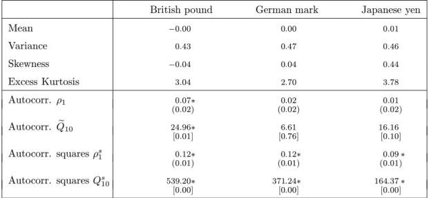
In table 1 we report some descriptive statistics of three exchange rate returns. The second part of this table analyzes the autocorrelation in the returns and their squares. Starting with the squared returns, the significant first-order autocorrelations point at conditional heteroskedasticity for all three series.7 Estimates for higher-order autocor-relations are not reported separately, but are combined in Box-Pierce type statistics
Qs10; they also indicate conditional heteroskedasticity.
As the autocorrelations of the squared returns suggest heteroskedasticity, we use heteroskedasticity-consistent standard errors for the autocorrelation statistics in the returns themselves. Only the British pound shows significant autocorrelation, which is completely due to the first-order coefficient. For that reason, we use a first-order autoregressive term in the mean equation (1) for the British pound.
6.2
Estimation Results
This subsection presents the estimation results for the regime-switching GARCH model. For comparison, we also estimate four other models. These benchmark models are two single-regime models, namely the constant variance model and the GARCH(1,1) mod-el, and two regime-switching ARCH models, namely the ARCH(0;0) and ARCH(4;4)
model. We use the notation ARCH(Q1;Q2) for a regime-switching model with Q1
ARCH terms in the first regime and Q2 in the second regime. The ARCH(4;4) model
is comparable with those of Cai (1994) and Hamilton and Susmel (1994). It is, however, somewhat more general, as the ARCH parameters are allowed to differ freely across regimes, whereas in Cai (1994) and Hamilton and Susmel (1994) the parameters only differ by an additive or multiplicative constant, respectively.
7
For all models we use a t-distribution instead of a normal one. In the regime-switching models we do this to make the persistence of regimes less sensitive to outliers, as will be explained below. For uniformity, we also use t-distributions in the single-regime models. The usefulness of t-distributed errors in the single-single-regime GARCH model has been shown in earlier studies, such as Engle and Bollerslev (1986).
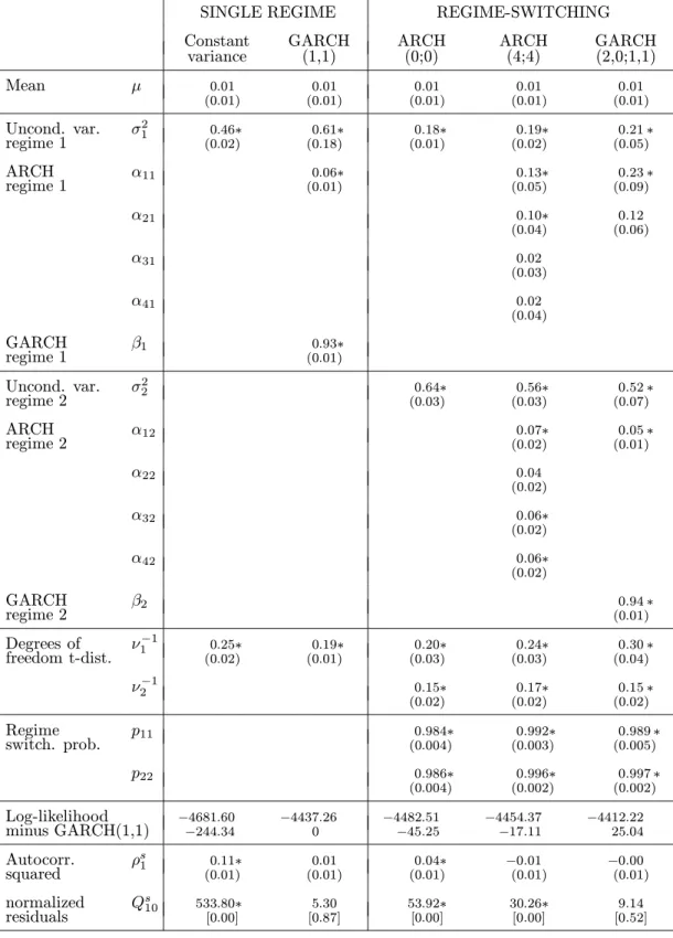
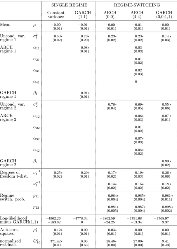
Tables 2, 3 and 4 present the maximum likelihood results for the British pound, German mark and Japanese yen, respectively. For easier comparison of the models, we present the ”unconditional” variances σ21=V{εt|rt= 1} and σ22=V{εt|rt= 2}
instead of the intercepts ω1 and ω2 in the conditional variance formula (4). They can
be computed with the formulas in appendix A. Moreover, we present the inverse of the degrees of freedom of the t-distribution; testing for conditional normality then boils down to testing whether ν−1 differs significantly from zero.
Single-regime GARCH
As is typically found, the standard, one-regime GARCH(1,1) model provides a much better fit than the constant variance model. For instance, the increase in log-likelihood of the GARCH model over the constant variance model is 244.34 for the British pound, so that ARCH and GARCH effects are statistically very important. Furthermore,
the sum of the ARCH and GARCH parameters (α+β) is large for all three series
pointing at high volatility persistence of individual shocks. This has also been found in earlier papers, for instance West and Cho (1995). Panel D of figures 1, 2 and 3 shows the estimated variance series Vbt−1{st} for the three series. The volatility persistence
appears from the gradual decrease of the conditional variance after a shock.
The high volatility persistence of shocks in the single-regime GARCH model may well indicate parameter instability, as we showed before. We estimate regime-switching models to analyze whether the high volatility persistence is indeed spurious.
Regime-switching ARCH(0;0)
Let us first consider the regime-switching ARCH(0;0) model in which persistence of regimes is the only source of volatility clustering. Tables 2, 3 and 4 show that all three regime-switching models clearly distinguish between a low and a high volatility regime, where the unconditional variance in the latter is about three times as large.
The variance regimes are also persistent, since the staying probabilitiesp11 andp22
are all above 0.975. To get a better idea about the amount of persistence that such staying probabilities imply, we compute the expected duration of the high variance
Hamilton (1989)) ∞ X l=1 l·P{rt= 2, . . . , rt+l−1= 2, rt+l= 1|rt= 2}= ∞ X l=1 l·(p22)l−1(1−p22) = (1−p22)−1.
For a typical ARCH(0;0) staying probability of 0.98, this implies an expected duration of 50 (working) days, which is about 2.5 months.
The introduction of variance regimes captures much of the volatility persistence in the data. To show this, we analyze the normalized residuals. Since in our model the variance depends on an unobserved regime, normalizing the residuals is not as easy as usual. One first has to integrate out the regime, as in (10). The square root of the resulting variance can then be used as the normalizing factor.
Tables 2, 3 and 4 present tests for heteroskedasticity in the normalized residual-s. The first-order autocorrelationsρs1 and the aggregate autocorrelation tests Qs10 for the squared normalized residuals show that the conditional heteroskedasticity in the normalized residuals has greatly reduced when going from the constant variance mod-el to the regime-switching modmod-el with constant regime-specific variances. However, the heteroskedasticity tests also make clear that there is still heteroskedasticity left. Apparently, there is also volatility clustering within a regime.
Regime-switching ARCH(4;4)
Cai (1994) and Hamilton and Susmel (1994) tried to capture the volatility clustering within regimes by ARCH dynamics. The heteroskedasticity tests for the yen show the usefulness of this approach. A regime-switching ARCH(4;4) model is sufficient to capture all conditional heteroskedasticity in the dollar-yen exchange rate returns, although at the cost of a number of extra parameters.
Allowing for only ARCH effects in a regime-switching model is, however, insufficient
for the two European currencies, as the aggregate autocorrelation testsQs10show. This
remaining conditional heteroskedasticity can be attributed to the high variance regime, as the ARCH(4;4) estimates for the high variance regime point at potentially longer persistence in the high variance regime only; for the low variance regime they show that even less than four ARCH terms would have been enough. Note that this also illustrates the importance of letting the ARCH parameters differ across regimes. This is in contrast with the models Cai (1994) and Hamilton and Susmel (1994) used, since they restricted the variances in both regimes to be the same apart from an additive of multiplicative scaling parameter, respectively.
An event that appeared to have a particularly long effect on the dollar-pound volatil-ity is the crash of the Exchange Rate Mechanism of the European Monetary System in
September, 1992 (see figure 1A). Taking only four lags is probably insufficient to gen-erate good conditional variance estimates for this period. The GARCH(1,1) estimated variance in figure 1D seems to capture the gradual decrease in volatility better than the ARCH(4;4) variance in figure 1G.
Regime-switching GARCH
The long persistence in the high volatility regime for the pound and the mark, as indicated by the ARCH(4;4) results, show the potential usefulness for GARCH terms as a parsimonious representation of the volatility persistence within regimes. Indeed, the sum of ARCH and GARCH parameters in the high volatility regime is large for the pound and the mark, and there is no heteroskedasticity left in the normalized residuals. Also the log-likelihood increases a lot after the introduction of GARCH terms in the high volatility regime: 42.15 for the pound and 22.71 for the mark. This shows that the persistence of individual shocks is largest in the dollar-pound exchange rate. For the yen this persistence is smallest, as the log-likelihood increase is -1.91.
Besides the volatility persistence within regimes, the regime-switching GARCH model also uses the regime-persistence as a source of volatility persistence. The per-sistence of regimes is illustrated by the plots of the estimated smoothed probability,
pT(rt), that the process is in the high variance regime (see panel B of figures 1, 2 and
3). We see that the two European currencies have experienced much less regime shifts than the Japanese yen. Apparently, sudden shifts in the variance are more important for the description of the yen than of the European currencies, where the conditional variance is more governed by smooth transitions (GARCH effects) from high volatility periods to low ones. This is also clear from the increase in the log-likelihood when introducing regime-specific GARCH effects to the ARCH(0;0) model, which has only regime-shifts to capture conditional heteroskedasticity. For the yen the increase is only 7.70, whereas for the pound it is 70.29 and for the mark 33.62.
An issue closely related to the persistence of regimes is the allowance for extra leptokurtosis by a t-distribution within a regime. Without this, the persistence of the, for example, low volatility regime would have been lower, since then a large sudden change in the exchange rate would have been considered earlier as a shift to the high volatility regime. This is illustrated by figure 1F, which gives the smoothed regime probabilities of the regime-switching GARCH model for the British pound under the restriction of normality. We see that under normality more regime-switches occur.
Comparing single-regime and multi-regime GARCH
So far, we have shown that regime-switching GARCH models are capable of captur-ing all volatility clustercaptur-ing, whereas regime-switchcaptur-ing ARCH models may fail. But standard, one-regime GARCH models also seem to capture the volatility clustering, at least according to the autocorrelation statistics in tables 2, 3 and 4. What is then the reason for introducing an extra source of volatility persistence by allowing for two regimes? Figure 1H shows the answer. This plot illustrates the essential difference be-tween single-regime and regime-switching GARCH models. It contains the conditional variance estimates of both GARCH models for the British pound for 1985 and 1986 only. The long effect of the largest shock in the data (March 27, 1985) on subsequen-t volasubsequen-tilisubsequen-ty appears subsequen-to be capsubsequen-tured well by bosubsequen-th models. However, subsequen-the sharp fall in the dollar one day after the G-5 Plaza announcement on September 22, 1985 is not dealt with correctly by the one-regime GARCH model. It overestimates the volatility after this event, because of the large volatility persistence of individual shocks. The regime-switching model, however, is able to capture this ”pressure relieving” effect, and will thus lead to better volatility forecasts in such periods. It can cut off the effect of large shocks in two ways. First, a switch from the high volatility to the low volatility regime leads to a sharp decrease in the variance. This regime-switch is also apparent from figure 1E, which plots the ex ante regime probabilitypt−1(rt−1) that the process
is in the high volatility regime. Secondly, after the regime-switch shocks have a much shorter effect, as the low volatility regime is also the low persistence regime. This sec-ond channel is only present if one does not restrict the GARCH parameters in both regimes to be equal. Given the large parameter differences, this channel appears to be an important way to forget large recent shocks.
In summary, our regime-switching GARCH model takes account of two significant aspects of exchange rate distributions, namely the occurrence of many large changes and the clustering of them. The first aspect is already captured in our constant variance model by the t-distribution for the innovations. This characteristic is also present in the four other models. For the second aspect, the clustering of large changes, the regime-switching GARCH model distinguishes two sources. The first one is the persistence of periods with different unconditional variances. This source is absent in the two single-regime models. Secondly, our model allows for volatility persistence even within regimes (in contrast with ARCH(0;0)) and allows for long-run persistence, which is in contrast with ARCH(4;4). In the next subsection we will analyze whether these model differences affect the forecast quality.
6.3
Forcasting Performance
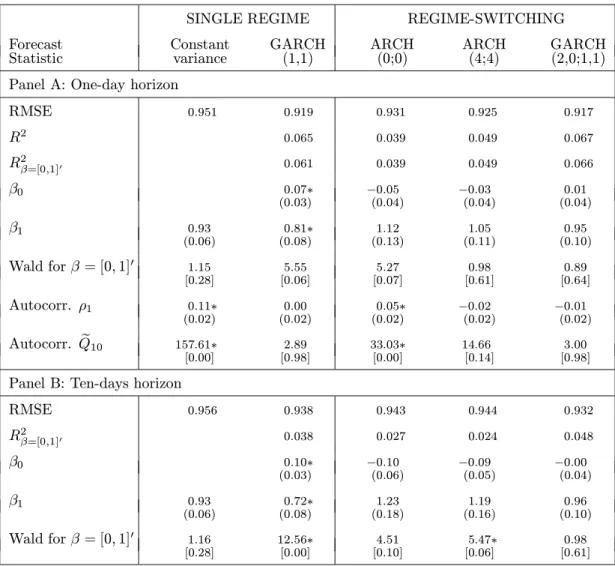
In this subsection we compare both the in-sample and out-of-sample forecasts generated by the five models discussed above. The forecasts are computed for two horizons, namely the one-day horizon, which corresponds to the data frequency, and the ten-days horizon.
In-sample forecasting
The in-sample forecasts at timet−1 of the variance of the return at some future timeτ, b
Vt−1{sτ}, follow from (10) after substitution of the estimation results of subsection 6.2.
Since the conditional variance is the conditional expectation of (sτ−µ)2, we compare
b
Vt−1{sτ}with (sτ−µb)2. We first take the one-day-ahead forecasts, so that τ=t.
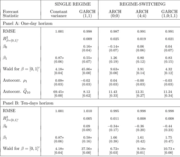
Following many other papers, such as Gray (1996a), the first forecast statistic we consider is the root mean squared error (RMSE), defined as the square root of
1 T PT t=1 (sτ −bµ)2−Vbt−1{sτ} 2
. From panel A of tables 5, 6 and 7 we see that the regime-switching GARCH model outperforms the standard, one-regime GARCH model
for all series.8 Apparently, the introduction of regimes into a GARCH model not only
leads to a better fit, but also to better forecasts.
We also see that for the British pound, the series with the highest volatility per-sistence of shocks, the outperformance of regime-switching GARCH over single-regime GARCH is smallest and that both our model and the single-regime GARCH model outperform the two regime-switching ARCH models. Apparently, in case of strong volatility persistence of individual shocks, taking account of this by GARCH terms is important. For the series with less volatility persistence of individual shocks, the dominance of our model over single-regime GARCH is larger, especially for the yen. Moreover, the forecasts generated by regime-switching GARCH and ARCH are of al-most equal quality. So, using regimes as a source of volatility persistence is particularly important if the persistence of individual shocks is not very large.
The conclusions continue to hold when we use another, often-used forecast statistic, namely the coefficient of determination,R2, of the regression
(sτ−µb)2 =β0+β1Vbt−1{sτ}+ητ. (12)
This regression is comparable with the ones used by Pagan and Schwert (1990). The quality difference between the regime-switching models and the single-regime GARCH model, however, seems smaller now.
8
The differences seem small, but relatively speaking they are substantial: the decrease in RMSE from the constant variance model to the single-regime GARCH model is enlarged by 6%, 21% and 117% for the pound, mark and yen, respectively, when going to the regime-switching GARCH model.
Using the R2 as a forecast statistic has one drawback. It measures the quality of a
linear combination, β0+β1Vbt−1{sτ}, of the forecast, although one is interested in the
quality of the forecast itself. Therefore, we prefer the quality measure
R2β=[0,1]0 = 1−
V n(sτ−µb)2−Vbt−1{sτ}
o
V{(sτ−µb)2} , (13)
which can be viewed as the R2 under the restriction that β
0 = 0 and β1= 1. This
forecast statistic is similar to the R2-type measure used by Gray (1996a). The tables
make clear that this change from R2 to R2β=[0,1]0 affects the quality measure for the
single-regime GARCH model by far the most. The reason for this will become clear below. The seemingly smaller difference between the regime-switching models and the single-regime GARCH model thus appears to be entirely due to an incorrect quality assessment. UsingR2β=[0,1]0 instead of the potentially misleadingR2confirms our earlier
conclusions based on the RMSE.
At first sight, it may seem that all models yield bad volatility forecasts, as the R2
statistics are quite low. However, as Andersen and Bollerslev (1997) argued, it is naive
to expect a ”high” R2 from regressions such as (12). They demonstrated that, even if
(sτ−µb)2 is a conditionally unbiased estimator of the variance of interest,Vt−1{sτ}, it is
a very noisy one, which leads to a low R2. Using better proxies for the latent variable
Vt−1{sτ}, they showed that (single-regime) GARCH models do provide good volatility
forecasts. Nevertheless, we find that regime-switching GARCH forecasts are better. As stated before, the relatively poor forecasting performance of standard, single-regime GARCH models may well be caused by the high volatility persistence of in-dividual shocks that we found in the previous subsection. Indeed, tables 5, 6 and 7 contain evidence for this claim. To explain this we analyze regression (12) again. If the mean and variance forecasts are (conditionally) unbiased, that is, µb =Et−1{sτ} and
b
Vt−1{sτ}=Vt−1{sτ}, then regression (12) implies thatβ0= 0 andβ1= 1 and that the
error terms ητ are serially uncorrelated.
The first two implications of the unbiasedness of the forecasts,β0= 0 andβ1= 1, are
tested both individually and simultaneously using OLS estimates for β0 and β1. For
reasons of uniformity, all tests are corrected for autocorrelation and heteroskedasticity.9 The individual tests are robust t-tests, whereas the simultaneous test is a Wald test using a robust estimate of the asymptotic covariance matrix of the OLS estimator for [β0, β1]0.
Tables 5, 6 and 7 make clear that the hypotheses are overwhelmingly rejected for the
9
In case of a ten-days forecast horizon the errors in (12) are no longer uncorrelated, so that the OLS standard errors have to be corrected; see also the notes below table 5.
single-regime GARCH model. All estimates forβ0 are significantly above zero, and all
but one estimates forβ1 are significantly below one. Apparently, the GARCH variance
estimates are too variable. Note that the rejection of [β0, β1]0 = [0,1]0 is exactly the
reason behind the large difference between the often-used, but potentially misleading unrestrictedR2 and the better forecast statisticR2β=[0,1]0 defined in (13).
Regarding the estimates forβ0 andβ1, all regime-switching models do much better,
since only one coefficient is significantly different from its hypothetical value. Therefore, not surprisingly, the Wald tests forβ= [0,1]0clearly prefer the regime-switching models over the single-regime GARCH model.
The crucial difference between the two types of models is that the regime-switching models have regimes as a means to capture volatility persistence, whereas single-regime GARCH models have to put all volatility persistence in the persistence of individual shocks. Given that the excessive variability of the forecasts disappears after the intro-duction of another way to capture volatility persistence, we conclude that it is the high persistence in single-regime GARCH models that makes the forecasts too variable.
To analyze the last implication of the unbiasedness of the forecasts, uncorrelated error terms ητ in (12), we compute the first-order autocorrelation in the residuals, ρ1,
and the (heteroskedasticity consistent) modified Box-Pierce statisticQe10 introduced in
table 1. The models that take most care of volatility clustering, standard GARCH, regime-switching ARCH(4;4) and GARCH, indeed show no significant autocorrelation. The highly significant values for ARCH(0;0) for the pound indicate once again that regime-switches alone are sometimes insufficient to capture all predictability of volatil-ity.
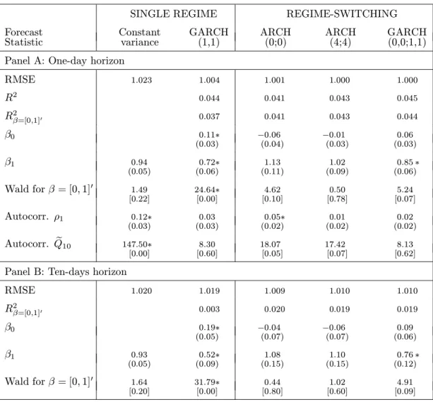
Panel B of tables 5, 6 and 7 presents statistics for the ten-days-ahead forecasts
(τ=t+9). Most conclusions for the one-week-ahead forecasts also apply here. So, again
the regime-switching GARCH model outperforms the single-regime GARCH model, es-pecially for series with moderate persistence of individual shocks. The regime-switching GARCH model also outperforms the regime-switching ARCH models in case of strong volatility persistence within regimes. Overall, our regime-switching GARCH model is thus the preferred model for in-sample forecasting. Note that the outperformance of the four heteroskedasticity models over the constant variance model is lower than for the one-day forecast horizon, as allR2
β=[0,1]0 are now closer to zero. Apparently, the longer
the forecast horizon, the less valuable is the information in the information setIt−1 for
forecasting. This is in line with the well-known fact that conditional heteroskedasticity is lower in lower-frequency data.
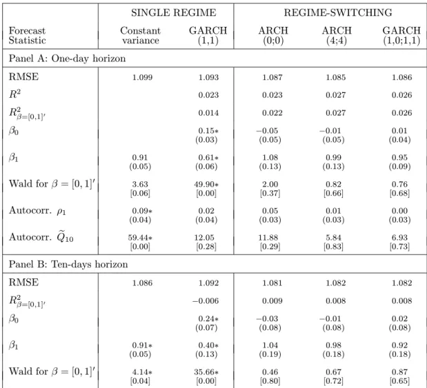
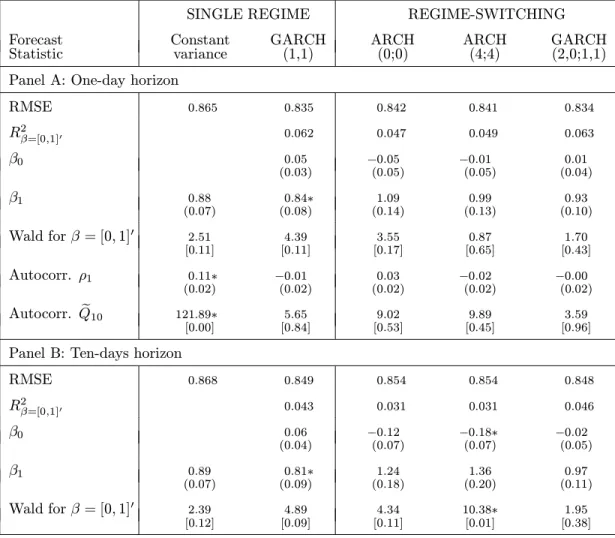
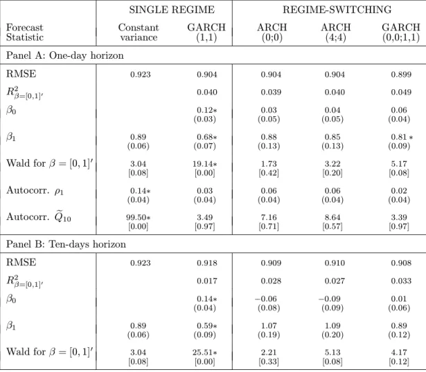
Out-of-sample forecasting
We now turn to the out-of-sample forecasts. We reestimate the five models for the three exchange rate returns using only the first half of the sample. Holding the parameters fixed, we then use the 2491 observations in the second half (from October 20, 1987 to July 12, 1997) to generate the volatility forecasts Vbt−1{sτ}.10 As before, we take the
one-day and ten-days horizons.
Tables 8, 9 and 10 show that the out-of-sample characteristics are similar to the in-sample ones. Single-regime GARCH models generate forecasts that are again too variable, which is not the case for the models that contain two variance regimes as
a second way to capture volatility persistence. Secondly, the RMSE and R2β=[0,1]0
demonstrate that the regime-switching GARCH model outperforms the standard, one-regime GARCH model, particularly in case of moderate volatility persistence of shocks, and that regime-switching GARCH again outperforms the two other regime-switching models for the British pound, which is the series with the highest persistence of shocks. The regime-switching forecasts for the other two series do not differ much, although the GARCH model is somewhat better for the German mark and ARCH(0;0) is slightly better for the Japanese yen.
7
Conclusion
Standard GARCH models often imply a lot of volatility persistence of individual shocks. We show that this makes the GARCH volatility forecasts too variable. Therefore, we extend the model such that shocks can, but need not be very persistent. This is achieved by the introduction of two regimes with different levels of volatility; a GARCH formula
is used to specify the variance within a regime. In the resulting regime-switching
GARCH model a shift from the high to the low variance regime can then explain that shocks are sometimes not persistent, but followed by a period of low instead of high volatility (”pressure relieving” effect). The empirical application using three U.S. dollar exchange rates shows the importance of regimes in a GARCH model: volatility forecasts improve substantially.
The ”pressure relieving” effect, however, can also be explained by regime-switching ARCH models; why need a GARCH term in the regime-specific variance? Regime-switching ARCH models were developed, because it seemed to be practically impossible to allow for long-run dependence in the conditional variance caused by a GARCH
10
We also did the reverse, that is, using the second half of the observations for estimation and the first half of the observations for forecasting. The conclusions are similar and will not be reported.
term. In this paper we present a way out of this problem by integrating out the unobserved regimes in a special way. Our empirical analysis demonstrates the usefulness of this: GARCH terms are important in regime-switching models and the quality of the volatility forecasts can benefit a lot from them.
Our third result is that volatility persistence is time-varying: in periods of high volatility shocks are more persistent than in periods of low volatility. Our model takes account of this by letting the ARCH and GARCH parameters differ across regimes. This time-varying volatility persistence reflects another way to decrease the effect of large shocks when necessary. A shift to the low variance regime after a large shock not only lowers the general volatility level, but it also implies a shift to the low persistence regime. Allowing for such effects appears to be empirically important.
As in other regime-switching models, the error distribution in our model is not restricted by normality; a t-distribution can be used as well. We show that this extra source of leptokurtosis is particularly useful in regime-switching models, since it makes the persistence of regimes less sensitive to outliers.
Another attractive feature of the model is that it yields simple, first-order recursive multi-period-ahead volatility forecasting formulas, similar to the ones for single-regime GARCH models. Moreover, estimation is also a first-order recursive process. Both properties make the model useful from a practical point of view.
Given the ease of generating volatility forecasts and that these forecasts outperform the often-used single-regime GARCH forecasts, the model has a number of possible applications. For example, the volatility forecasts can be used to analyze the effect of volatility on stock returns. Moreover, they may be helpful to price options, where volatility assessments are crucial. Both applications are left for future work.
Appendices
A
Unconditional Error Variance
Suppose the ”unconditional” variance V{εt|rt} exists for all rt= 1,2 and ω1, ω2 >0.
Using the variance definition (4), repeated use of the law of iterated expectations yields
V{εt|rt} =ωrt+αrtE{ε 2 t−1|rt}+βrtE{Vt−2{εt−1|rt−1}|rt} =ωrt+αrtE{E{ε 2 t−1|rt−1, rt}|rt}+βrtE{E{Vt−2{εt−1|rt−1}|rt−1, rt}|rt} =ωrt+αrtE{V{εt−1|rt−1}|rt}+βrtE{V{εt−1|rt−1}|rt} =ωrt+ (αrt+βrt)·E{V{εt−1|rt−1}|rt}, (14)
where the penultimate equality uses that the distribution of the error given the
contem-poraneous variance regime does not depend on the future variance regimert. Assuming
that εt|rt is unconditionally homoskedastic, stackingV{εt|rt= 1} and V{εt|rt= 2}
yields V{εt|rt= 1} V{εt|rt= 2} = ω1 ω2 + A1|1 A2|1 A1|2 A2|2 · V{εt|rt= 1} V{εt|rt= 2} , (15) whereAi|j =P{rt−1=i|rt=j}(αj+βj). Expressions for the probabilities involved are
given in appendix B. LetA be the matrix with elements Ai|j. Since we have assumed
that both unconditional variances exist, I2 −A is invertible. We get the following
one-to-one relation between the unconditional variances and the vector of ω1 and ω2:
V{εt|rt= 1} V{εt|rt= 2} = (I2−A)−1· ω1 ω2 (16)
To obtain necessary conditions for the existence of both variances, we use A2|1 =
α1+β1−A1|1 and A1|2=α2+β2−A2|2 to rewrite (I2−A)−1 as (I2−A)−1= 1 det(I2−A) 1−A2|2 α1+β1−A1|1 α2+β2−A2|2 1−A1|1 . (17) Since the variances are strictly positive for allω1, ω2 >0, the four elements of (I2−A)−1
for both regimes i= 1,2, this implies that det(I2−A) >0, so that 1−A1|1 ≥0 and
1−A2|2 ≥0. However, neitherA1|1 norA2|2 may be unity; otherwiseαi+βi−Ai|i ≥0
for both regimes would imply that det(I2−A)<0, which is not the case.
In summary, we have three necessary conditions for the existence of the ”uncon-ditional” variances V{εt|rvt}, namely A1|1, A2|2 < 1 and det(I2 −A) > 0. So, two
linear combinations of the regime-specific ARCH and GARCH coefficients must be less than one and there is some restriction on the combination of the coefficients of both
equations. These are similar to the necessary (and sufficient) condition α+β < 1 in
the standard, one-regime GARCH(1,1) model.
B
Regime Probabilities
In section 3 we have to compute the densitypt−1(st) in (7). This requirespt−1(rt) and
pt−1(rt−1|rt), where the latter is needed to compute the expectation in the variance
Vt−1{εt|rt} given by (9). The first probability can be rewritten as
pt−1(rt) =
X
rt−1=1,2
pt−1(rt−1)·pt−1(rt|rt−1), (18)
where the constant switching probabilitypt−1(rt|rt−1) follows from (6).
The second probability needed above is
pt−1(rt−1|rt) =
pt−1(rt−1)·pt−1(rt|rt−1)
pt−1(rt)
, (19)
wherept−1(rt) is given by (18).
Formulas (18) and (19) show that both regime probabilities in section 3 can be com-puted from one key probabilitypt−1(rt−1). This probability has a first-order recursive
structure.
Recursion for Key Probability
The key probability can be written aspt−1(rt−1) = pt−2(rt−1 |st−1) = pt−2(st−1|rt−1)·pt−2(rt−1) pt−2(st−1) (20) = pt−2(st−1|rt−1)· P rt−2=1,2pt−2(rt−2)·pt−2(rt−1|rt−2) pt−2(st−1) (21) Because the switching probabilitypt−2(rt−1|rt−2) is constant, the only variables needed
to compute the basic probability are the previous key probability pt−2(rt−2) and the
previous densities pt−2(st−1|rt−1) and pt−2(st−1). This makes the computation of the
Regime Probabilities for Forecasting
Section 5 deals with forecasting l-periods-ahead exchange rate returns sτ, where τ=
t−1+l≥t. For their variance, Vt−1{sτ}, we need in (10)
pt−1(rτ) =
X
rt−1=1,2
pt−1(rt−1)·pt−1(rτ |rt−1), (22)
where pt−1(rt−1) is the key probability discussed above. For the multi-period-ahead
probability on the right-hand-side of (22), we form the time-constant Markov variance
regime transition matrixM:
M = p11 1−p22 1−p11 p22 . (23)
Using thel-th power ofM, the theory of Markov processes states that
pt−1(rτ |rt−1) =
Ml
rτ rt−1
. (24)
To compute the varianceVt−1{ετ|rτ}in (11), where τ exceeds t, we need
pt−1(rτ−1|rτ) =
pt−1(rτ |rτ−1)·pt−1(rτ−1)
pt−1(rτ)
. (25)
The switching probability follows from (6) and the regime probabilitypt−1(rτ−1) follows
in a similar way as pt−1(rτ) in (22); the denominator is given by (22).
Regime Probabilities in Unconditional Variance
In appendix A we need some unconditional probabilities to compute the unconditional error variance in (15). Using Bayes’ rule, we have
p(rt−1|rt) =
p(rt|rt−1)·p(rt−1)
P
rt−1=1,2p(rt|rt−1)·p(rt−1)
, (26)
where p(rt|rt−1) is constant (see (6)) and the theory of Markov processes gives the
unconditional probabilities (see Hamilton (1989)):
p(rt−1= 1) = 1−p22 2−p11−p22 p(rt−1= 2) = 1−p11 2−p11−p22 . (27)
C
Ex Post Regime Probabilities
As stated in section 4, the ex post regime probability pτ(rt), for a given future time
τ ∈ {t, t+ 1, . . . , T}, can be computed recursively, starting from the ex ante probability
pt−1(rt).
We can write pτ(rt) for both regimesrt= 1,2 as
pτ(rt) =pτ−1(rt|sτ)
= P pτ−1(sτ|rt)·pτ−1(rt)
rt=1,2pτ−1(sτ|rt)·pτ−1(rt)
, (28)
where pτ−1(rt) is known from the previous recursion for all rt= 1,2, ifτ > t. If τ=t,
it is known from the estimation process, since then it is simply the ex ante probability given by (18).
The second ingredient of (28) is the density pτ−1(sτ|rt) for both regime outcomes.
For τ =t it is known from the estimation process (see (8) and (9)), so that the filter
probability, pt(rt), follows directly from (28). Therefore, let us suppose from now on
that τ > t. Computing pτ−1(sτ|rt) requires a number of steps. We first write it as
pτ−1(sτ|rt) =
X
rτ=1,2
pτ−1(sτ|rτ)·pτ−1(rτ|rt), (29)
where we use that the conditional distribution of sτ givenrτ does not depend on the
earlier regime rt. This formula itself has two ingredients. The first one is the density
pτ−1(sτ|rτ) for all regime combinations, which is known from the estimation process.
The second term needed in (29) is the (τ−t)-period-ahead regime-switching
prob-ability pτ−1(rτ|rt) for all regime outcomes. Once it has been computed, it should be
saved, since it will be needed in the next recursive step. Making use of the Markov
structure of the regime process, it can be written in terms of (τ−1−t)-period-ahead
switching probabilities
pτ−1(rτ|rt) =
X
rτ−1=1,2
pτ−1(rτ|rτ−1)·pτ−1(rτ−1|rt). (30)
Again we have two ingredients. First, we need pτ−1(rτ|rτ−1) for all regime
combina-tions. These are constant and follow from (6).
The second ingredient of (30) ispτ−1(rτ−1|rt) for all regime combinations. We have
pτ−1(rτ−1|rt) =pτ−2(rτ−1|rt, sτ−1)
= P pτ−2(sτ−1|rτ−1)·pτ−2(rτ−1|rt)
rτ−1=1,2pτ−2(sτ−1|rτ−1)·pτ−2(rτ−1|rt)
where we use that the conditional density ofsτ−1is independent of the earlier regimert
oncerτ−1is given. We have two ingredients. First, the conditional densitypτ−2(sτ−1|rτ−1)
for both regime outcomes. It is known from the estimation process. Secondly, we need the (τ−1−t)-period-ahead switching probabilitypτ−2(rτ−1|rt) for all regime
combina-tions. This one was saved during the previous recursion, if τ > t+ 1. If τ=t+ 1, it equals one.
This completes the algorithm to compute (29), which is the second ingredient of (28). For each recursion one has to compute (31), use the result to compute (30) and use this to compute (29). Using this in (28) yields the ex post probabilitypτ(rt) from
pτ−1(rt). Therefore, starting from the ex ante probabilitypt−1(rt) one can recursively
compute the ex post probabilitypτ(rt).
D
Recursive Formula for Conditional Variance of Future
Error
In this appendix we prove the recursive formula (11), which is needed for forecasting. It states
Vt−1{ετ|rτ}=ωrτ + (αrτ +βrτ)Et−1{Vt−1{ετ−1|rτ−1}|rτ}, (32)
where, for notational convenience, the index t+i has been substituted by τ. This
formula can be proved by repeatedly using the law of iterated expectations. Using definition (4), we get Vt−1{ετ|rτ}=Et−1[Vτ−1{ετ|rτ} |rτ] =Et−1 h ωrτ +αrτε2τ−1+βrτEτ−1{Vτ−2{ετ−1|rτ−1}|rτ} |rτ i (33) For the ARCH part we get
Et−1[ε2τ−1 |rτ] =E{ε2τ−1|rτ, It−1}
=E[E{ε2τ−1|rτ−1, rτ, It−1} |rτ, It−1]
=Et−1[Et−1{ε2τ−1|rτ−1} |rτ], (34)
where the last equality uses that the error distribution given the contemporaneous variance regime does not depend on the future variance regime.
For the GARCH part we use similar techniques to obtain Et−1[Eτ−1(Vτ−2{ετ−1|rτ−1} |rτ)|rτ] =E[E(V{ετ−1|rτ−1, Iτ−2} |rτ, Iτ−1)|rτ, It−1] =E(V{ετ−1|rτ−1, Iτ−2} |rτ, It−1) =E[E(V{ετ−1|rτ−1, Iτ−2} |rτ, rτ−1, It−1) |rτ, It−1] =E[V{ετ−1|rτ−1, It−1} |rτ, It−1] =Et−1[Vt−1{ετ−1|rτ−1} |rτ]. (35)
The penultimate equality uses thatIτ−2 givenrτ, rτ−1, It−1 is independent ofrτ, since
the Markov structure implies that the distribution of variance regimes ..., rτ−3, rτ−2
conditional on rτ−1 and rτ is independent of rτ; this makes the returns ..., sτ−3, sτ−2
also independent ofrτ oncerτ−1 and rτ are given.
Substituting the results for the ARCH and GARCH parts in (33) gives formula (32).
References
Andersen T.G. and T. Bollerslev (1997), ”Answering the Critics: Yes, ARCH Models Do Provide Good Volatility Forecasts,” NBER Working Paper No. 6023.
Bollerslev, T. (1986), ”Generalized Autoregressive Conditional Heteroskedasticity,”
Journal of Econometrics, 31, 307-327.
Bollerslev, T., R.Y. Chou and K.F. Kroner (1992), ”ARCH Modeling in Finance,”
Journal of Econometrics, 52, 5-59.
Cai, J. (1994), ”A Markov Model of Unconditional Variance in ARCH,” Journal of
Business and Economic Statistics, 12, 309-316.
Engle, R.F. (1982), ”Autoregressive Conditional Heteroskedasticity with Estimates of
the Variance of U.K. Inflation,”Econometrica, 50, 987-1008.
Engle, R.F. and T. Bollerslev (1986), ”Modeling the Persistence of Conditional
Vari-ances,”Econometric Reviews, 5, 1-50.
Gray, S.F. (1996a), ”Modeling the Conditional Distribution of Interest Rates as a
Regime-Switching Process,” Journal of Financial Economics, 42, 27-62.
Gray, S.F. (1996b), ”An Analysis of Conditional Regime-Switching Models,” Working Paper, Fuqua School of Business, Duke University.
Hakkio, C.S. and M. Rush (1989), ”Market Efficiency and Cointegration: an
Applica-tion to the Sterling and Deutschemark Exchange Markets,” Journal of
Interna-tional Money and Finance, 8, 75-88.
Hamilton, J.D. (1989), ”A New Approach to the Economic Analysis of Nonstationary
Time Series and the Business Cycle”, Econometrica, 57, 357-384.
Hamilton, J.D. and R. Susmel (1994), ”Autoregressive Conditional Heteroscedasticity
and Changes in Regime,” Journal of Econometrics, 64, 307-333.
Lamoureux, C.G. and W.D. Lastrapes (1990), ”Persistence in Variance, Structural
Change, and the GARCH Model,” Journal of Business and Economic Statistics,
8, 225-234.
Newey, W.K. and K.D. West (1987), ”A Simple, Positive Semi-definite,
Heteroskedas-ticity and Autocorrelation Consistent Covariance Matrix,”Econometrica, 55,
Newey, W.K. and K.D. West (1994), ”Automatic Lag Selection in Covariance Matrix
Estimation,”Review of Economic Studies, 61, 631-653.
Pagan, A.R. and G.W. Schwert (1990), ”Alternative Models for Conditional Stock Volatility,”Journal of Econometrics, 45, 267-290.
West, K.D. and D. Cho (1995), ”The Predictive Ability of Several Models of Exchange
Rate Volatility,”Journal of Econometrics, 69, 367-391.
White, H. (1980), ”A Heteroskedasticity-Consistent Covariance Matrix Estimator and
Table 1: Moments of exchange rate returns and autocorrelation tests.
British pound German mark Japanese yen
Mean −0.00 0.00 0.01 Variance 0.43 0.47 0.46 Skewness −0.04 0.04 0.44 Excess Kurtosis 3.04 2.70 3.78 Autocorr. ρ1 0.07∗ 0.02 0.01 (0.02) (0.02) (0.02) Autocorr. Qe10 24.96∗ 6.61 16.16 [0.01] [0.76] [0.10] Autocorr. squaresρs 1 0.12∗ 0.12∗ 0.09∗ (0.01) (0.01) (0.01) Autocorr. squaresQs 10 539.20∗ 371.24∗ 164.37∗ [0.00] [0.00] [0.00]
Standard errors in parentheses and p-values in square brackets; * is significant at 5% level.
The first-order autocorrelation, ρ1, is estimated as the slope coefficient in a regression of the return,
st, on the first lagged return,st−1, and a constant. The standard errors are based on White’s (1980)
heteroskedasticity-consistent asymptotic covariance matrix. e
Q10denotes a modified Box-Pierce type statistic that combines the first ten autocorrelations. Following
Pagan and Schwert (1990), it is defined as the sum of the first ten squared normalized autocorrelation estimates, where the normalizing factors are the heteroskedasticity-consistent standard errors of the autocorrelation estimates. Qe10is asymptoticallyχ210distributed.
The first-order autocorrelation in the squared returns, ρs
1, and the Box-Pierce type statistic Qs10 are
Table 2: Estimation results for the British pound.
SINGLE REGIME REGIME-SWITCHING
Constant GARCH ARCH ARCH GARCH
variance (1,1) (0;0) (4;4) (2,0;1,1) Mean µ 0.01 0.01 0.01 0.01 0.01 (0.01) (0.01) (0.01) (0.01) (0.01) Uncond. var. σ2 1 0.46∗ 0.61∗ 0.18∗ 0.19∗ 0.21∗ regime 1 (0.02) (0.18) (0.01) (0.02) (0.05) ARCH α11 0.06∗ 0.13∗ 0.23∗ regime 1 (0.01) (0.05) (0.09) α21 0.10∗ 0.12 (0.04) (0.06) α31 0.02 (0.03) α41 0.02 (0.04) GARCH β1 0.93∗ regime 1 (0.01) Uncond. var. σ2 2 0.64∗ 0.56∗ 0.52∗ regime 2 (0.03) (0.03) (0.07) ARCH α12 0.07∗ 0.05∗ regime 2 (0.02) (0.01) α22 0.04 (0.02) α32 0.06∗ (0.02) α42 0.06∗ (0.02) GARCH β2 0.94∗ regime 2 (0.01) Degrees of ν1−1 0.25∗ 0.19∗ 0.20∗ 0.24∗ 0.30∗ freedom t-dist. (0.02) (0.01) (0.03) (0.03) (0.04) ν2−1 0.15∗ 0.17∗ 0.15∗ (0.02) (0.02) (0.02) Regime p11 0.984∗ 0.992∗ 0.989∗ switch. prob. (0.004) (0.003) (0.005) p22 0.986∗ 0.996∗ 0.997∗ (0.004) (0.002) (0.002) Log-likelihood −4681.60 −4437.26 −4482.51 −4454.37 −4412.22 minus GARCH(1,1) −244.34 0 −45.25 −17.11 25.04 Autocorr. ρs1 0.11∗ 0.01 0.04∗ −0.01 −0.00 squared (0.01) (0.01) (0.01) (0.01) (0.01) normalized Qs 10 533.80∗ 5.30 53.92∗ 30.26∗ 9.14 residuals [0.00] [0.87] [0.00] [0.00] [0.52]
Standard errors in parentheses and p-values in square brackets; * is significant at 5% level. Both autocorrelation statistics have been defined below table 1.
For uniformity with other tables we do not report the first-order autoregressive coefficient that was estimated for the pound only.
Table 3: Estimation results for the German mark.
SINGLE REGIME REGIME-SWITCHING
Constant GARCH ARCH ARCH GARCH
variance (1,1) (0;0) (4;4) (0,0;1,1) Mean µ −0.00 −0.01 −0.00 −0.01 −0.00 (0.01) (0.01) (0.01) (0.01) (0.01) Uncond. var. σ2 1 0.50∗ 0.70∗ 0.23∗ 0.23∗ 0.14∗ regime 1 (0.02) (0.20) (0.02) (0.02) (0.03) ARCH α11 0.08∗ 0.03 regime 1 (0.01) (0.03) α21 0.01 (0.02) α31 0.02 (0.03) α41 0 GARCH β1 0.91∗ regime 1 (0.01) Uncond. var. σ22 0.76∗ 0.69∗ 0.55∗ regime 2 (0.04) (0.05) (0.06) ARCH α12 0.06∗ 0.07∗ regime 2 (0.03) (0.01) α22 0.01 (0.02) α32 0.07∗ (0.03) α42 0.05∗ (0.02) GARCH β2 0.90∗ regime 2 (0.02) Degrees of ν1−1 0.25∗ 0.20∗ 0.17∗ 0.19∗ 0.26∗ freedom t-dist. (0.02) (0.01) (0.02) (0.03) (0.06) ν2−1 0.14∗ 0.15∗ 0.18∗ (0.02) (0.02) (0.02) Regime p11 0.984∗ 0.985∗ 0.981∗ switch. prob. (0.004) (0.004) (0.011) p22 0.981∗ 0.987∗ 0.998∗ (0.005) (0.004) (0.002) Log-likelihood −4962.26 −4778.34 −4802.59 −4791.68 −4768.97 minus GARCH(1,1) −183.92 0 −24.25 −13.34 9.37 Autocorr. ρs1 0.12∗ 0.00 0.03∗ −0.00 0.00 squared (0.01) (0.01) (0.01) (0.01) (0.01) normalized Qs10 371.42∗ 8.03 28.46∗ 27.00∗ 9.41 residuals [0.00] [0.63] [0.00] [0.00] [0.49]
Standard errors in parentheses and p-values in square brackets; * is significant at 5% level. A 0 indicates a boundary solution.
Table 4: Estimation results for the Japanese yen.
SINGLE REGIME REGIME-SWITCHING
Constant GARCH ARCH ARCH GARCH
variance (1,1) (0;0) (4;4) (1,0;1,1) Mean µ −0.01 −0.01 −0.01 −0.01 −0.01 (0.01) (0.01) (0.01) (0.01) (0.01) Uncond. var. σ12 0.50∗ 0.61∗ 0.23∗ 0.26∗ 0.24∗ regime 1 (0.03) (0.11) (0.02) (0.03) (0.03) ARCH α11 0.09∗ 0.08∗ 0.08 regime 1 (0.02) (0.04) (0.05) α21 0 α31 0.05 (0.03) α41 0.02 (0.03) GARCH β1 0.87∗ regime 1 (0.02) Uncond. var. σ2 2 0.71∗ 0.68∗ 0.64∗ regime 2 (0.04) (0.04) (0.05) ARCH α12 0.04 0.06∗ regime 2 (0.03) (0.02) α22 0.05 (0.03) α32 0.05 (0.03) α42 0.01 (0.02) GARCH β2 0.78∗ regime 2 (0.10) Degrees of ν1−1 0.28∗ 0.25∗ 0.23∗ 0.25∗ 0.26∗ freedom t-dist. (0.02) (0.02) (0.03) (0.03) (0.03) ν2−1 0.17∗ 0.17∗ 0.18∗ (0.02) (0.02) (0.02) Regime p11 0.976∗ 0.982∗ 0.977∗ switch. prob. (0.007) (0.006) (0.008) p22 0.975∗ 0.982∗ 0.983∗ (0.006) (0.005) (0.005) Log-likelihood −4794.20 −4682.58 −4672.19 −4662.58 −4664.49 minus GARCH(1,1) −111.62 0 10.39 20.00 18.09 Autocorr. ρs 1 0.09∗ 0.02 0.04∗ 0.01 0.01 squared (0.01) (0.01) (0.01) (0.01) (0.01) normalized Qs 10 164.36∗ 13.02 21.57∗ 11.11 11.74 residuals [0.00] [0.22] [0.02] [0.35] [0.30]
Standard errors in parentheses and p-values in square brackets; * is significant at 5% level. A 0 indicates a boundary solution.