A SHORT-TERM ENSEMBLE WIND-SPEED FORECASTING SYSTEM FOR WIND POWER APPLICATIONS
BY
JUSTIN JOSEPH TRAITEUR
THESIS
Submitted in partial fulfillment of the requirements for the degree of Master of Science in Atmospheric Sciences
in the Graduate College of the
University of Illinois at Urbana-Champaign, 2011
Urbana, Illinois
Adviser:
ii Abstract
Accurate short-term wind speed forecasts for utility-scale wind farms will be crucial for the U.S. Department of Energy’s (DOE) goal of providing 20% of total power from wind by 2030. For typical pitch-controlled wind turbines, power output varies as the cube of wind speed over a significant portion of the power output curve. Therefore, small improvements in wind-speed forecasts would constitute much larger improvements in wind power forecasts. In addition, communicating the level of uncertainty in these wind speed forecasts will allow the industry to better quantify the level of financial risk inherent with these forecasts. In this study, a computationally efficient and accurate forecasting system is developed. This system uses a
21-member ensemble of the Weather Research and Forecasting Single-Column Model (WRF-SCM V3.1.1) to generate a probability distribution function (PDF) of 1-hour forecasts at a 90m height location in West/Central Illinois. The WRF-SCM ensemble was initialized by the 20 km Rapid update Cycle (RUC) 00h forecast and perturbed by both perturbations in the initial conditions and physics options. The PDF was calibrated using Bayesian Model Averaging (BMA) where the individual forecasts were weighted according to their
performance. This combination of a mesoscale numerical weather prediction ensemble system and Bayesian statistics allowed for both accurate prediction of 1-hour wind speed forecasts and their level of uncertainty.
iii Acknowledgements
I would like to thank my advisor, Dr. Somnath Baidya Roy, who has been extremely patient and helpful, as I have matured as a graduate student. Somnath has allowed me to be a second author on a previous paper and first author for my thesis research. I would also like to thank my family and friends who have supported me through the difficulties of graduate life. Finally, I would like to thank Karen O’Brien for the tremendous strength and support she has given me throughout my entire college career.
iv TABLE OF CONTENTS
1. INTRODUCTION ...1
1.1 Current Forecasting Techniques...5
1.2 Ensemble Forecasting with Bayesian Model Averaging ...8
1.3 Research Question ... 11 2. METHODS... 12 2.1 Study Site ... 12 2.2 Time Period ... 14 2.3 WRF-SCM Ensemble... 17 2.4 BMA Calibration... 22
2.5 Forecast Quality Control ... 29
2.6 Observation Quality Control ... 30
2.7 Forecast Evaluation... 30
3. RESULTS ... 34
3.1 Example Forecast ... 34
3.2 Calibrated vs. Uncalibrated Ensemble ... 34
3.3 RUC Model Bias Effects... 38
3.4 Calibrated Ensemble Member Performance... 40
3.5 Convective Daytime Regime... 40
3.6 Stable Nocturnal and Transition Regimes ... 41
3.7 Training Window Sensitivity ... 43
4. CONCLUSIONS AND DISCUSSIONS ... 46
5. FUTURE WORK... 50
1 1. INTRODUCTION
In order for wind power to be a viable solution to the global carbon and fossil fuel problem, accurate forecasts of wind speed will be vital for the growth of the wind power industry. Errors in wind speed forecasts lead to errors in forecasting for both demand of electricity and power supply from wind farms [McSharry et al., 2005]. For typical pitch-controlled wind turbines, power output varies as the cube of wind speed over a significant portion of the power output curve (Figure 1.1). Therefore, small improvements in wind-speed forecasts constitute much larger improvements in wind power forecasts. A 10%-20%
improvement in wind power generation forecasts equates to hundreds of millions to billions of dollars in savings in annual operating costs. Since power output of a wind farm is a function of the wind-speed, power generation can vary from timescales of less than a minute to several days or weeks [Lew et al., 2010]. The wind power industry thus needs accurate wind-speed forecasts for the timescale of several
minutes to several years for a wide range of applications including
turbine blade pitch control, conversion systems control, load scheduling, maintenance scheduling and resource planning [Stetsos, 2000; Costa et al., 2008]. Errors in the application of these processes constitute
2
Figure 1.1 The top figure shows a power curve for a Gamesa 2 MW wind turbine. The cut-in speed at which the turbine starts to produce power is 4 m/s, the cut-out speed or the furling speed, which is the wind speed at which the machine shuts down to avoid damage is 25m/s. The bottom figure is the amount of power produced compared to the theoretical limit. At low wind speeds the machine is very efficient at capturing energy from the flow but decreases as the wind approaches the cut-out speed.
3
Accurate wind forecasts are of particular importance to the U.S. wind power industry. The U.S. Department of Energy’s (DOE) goal of providing 20% of total power from wind by 2030 is considered an Engineering Grand Challenge. In order to reach the goal of 20% wind power penetration, wind power installations would need to increase to more than 16,000 MW per year by 2018 and continue at that rate until 2030 [USDOE, 2008]. At such a high level of market penetration, wind farms must be integrated with the grid [Georgilakis, 2008]. To
accomplish this task, wind farms must guarantee a fixed amount of electricity generation over different time scales [Smith et al., 2004]. Over the short-medium time horizon, the following 3 timescales are of interest for operation of the utility system and the structure of the competitive electricity markets [Smith et al., 2004]:
• Unit-commitment horizon of 1 day to 1 week
• Load-following horizons of 1 to several hours
• Regulation-horizon of 1 minute to 1 hour
The unit-commitment time frame encompasses decisions
regarding the scheduling of unit startup and shutdown while retaining system reliability at minimum cost. If the wind farm deviates from their
4
day ahead schedules by more that ±1.5% then financial penalties are imposed under FERC 888 [NARUC, 2007].
The load-following time frame spans from 1 to several hours in length. In this time frame, utilities must be able to ramp units up and down to follow the load resulting from random fluctuations in the combined load and wind plant output.
The focus of this paper is to develop a wind speed forecasting system for the regulation horizon. In the regulation horizon time frame, sufficient regulating capacity must be available from the units on
regulating duty to hold deviations within the tolerance prescribed by the North American Electric Reliability Council. The statistically accepted deviations are quantified in the Control Performance Standards 1 and 2 (CPS-1 and CPS-2) [Smith et al., 2004]. Only with accurate wind speed forecasts that can also predict ramp up and down events at the 1-hour level or less will the problem of the regulation scheduling diminish.
5 1.1 Current Forecasting Techniques
Currently, many forecasting techniques exist for short-term forecasting of wind speed at the 1-hour level. Numerical Weather Prediction (NWP), statistical models, and artificial neural networks (ANN) can be used individually or in concert with each other to provide wind speed forecasts. A brief discussion of each forecasting technique is discussed in the next few paragraphs.
NWP has recently been the major focus of the literature for wind speed prediction. NWP models operate by solving a system of
3-dimensional conservation equations of mass, momentum and energy in the atmosphere at given locations on a spatial grid. They also include subgrid-scale turbulent transfer and microphysical processes. The models are initialized by observations taken both in situ and remotely. The numerical model then solves the system of equations to provide a forecast of temperature, wind velocity, pressure and precipitation for a future time. NWP models are very complex and can take minutes to hours to complete. The more sophisticated models require a large computing infrastructure and are typically run by large governmental agencies such as the Global Forecast System (GFS) at the National Center for Atmospheric Research (NCEP).
6
A major factor that influences the accuracy of the NWP models is the resolution of the grid and uncertainty in the initial observations and parameterization schemes. Finer spatial grid spacing than general forecasting NWP models, such as the GFS, is needed in order to provide sufficient results for wind speed power forecasting. These higher
resolution models are able to better capture the smaller-scale
atmospheric and geographic features that are inherently different at each forecast site. For any numerical model, a minimum of five grid points are required to resolve a wave’s structure. Therefore only NWP models of at least 20 km resolution or less can adequately capture mesoscale atmospheric structures.
Deterministic single-valued forecasts from NWP models contain uncertainties primarily due to errors in model initialization and/or model imperfections in parameterization schemes and resolution. These
uncertainties can be minimized by conducting ensemble simulations where multiple forecasts are generated by (i) adding small
perturbations to the initial conditions; (ii) using different
parameterizations for geophysical processes; (iii) using multiple models [Molteni et al., 1996; Toth and Kalnay, 1997; Buizza et al., 2005]. The ensemble mean can now be considered the most likely forecast [Buizza, et al., 1999; Palmer 2000]. Recent studies have proposed
7
improvements over the conventional ensemble averaging method. Linear averaging of outputs from individual ensemble members
assumes that the individual forecasts are equiprobable and hence can underestimate uncertainty [Taylor, 2004; Taylor and Buizza, 2006]. To improve the quantification and further reduce the effects of uncertainty, the individual ensembles can be calibrated against observations.
While NWP models solve a set of prognostic equations to forecast the future state of the atmosphere, statistical models predict the future of several meteorological variables based on past events at the forecast site. These models study the past spatial-temporal evolution of
weather variables such as wind, temperature and pressure to discover patterns relative to each other at a given site. There are a wide range of methods employed for statistical forecasting such as linear and non-linear regression, autoregressive model, moving average model,
autoregressive average model, autoregressive integrated moving average model, kalman filter, spatial correlation method and
persistence [Duran et al., 2007; Costa et al., 2008; Riahy and Duran, 2008; Lei et al., 2009; Taylor et al., 2009]. This forecasting technique has shown promising results for forecasting timescales less than several hours in length.
8
Another forecasting technique used by wind farm operators incorporates the use of Artificial Neural Networks (ANN). Artificial Neural Networks are very similar to other statistical techniques in that they used for very short forecasting time periods (<3 hours) and learn from the difference between NWP forecasts and observations. There are some important differences however. While most statistical methods are auto-recursive, i.e. use the difference between the predicted and actual wind speeds immediately past to tune the
parameters in the model, ANN use past data taken over a given time-frame to learn the relationships between the input data and output wind speeds to learn historic patters in order to predict future patterns. Since it is increasingly difficult to obtain measurements that are highly correlated to the long-term wind forecast, the accuracy of these models degrades with increasing prediction time. Therefore, NWP models will be needed in order to give accurate wind power forecasts for
increasingly longer timescales [Potter et al., 2004].
1.2 Ensemble Forecasting With Bayesian Model Averaging
NWP models can sometimes have an advantage over statistical and ANN models forecasting systems. Since statistical models only
9
predict the future state of the atmosphere by looking at the past, they commonly fail when a component of the atmosphere is changing. For example, empirically identified relationships that govern wind speed are likely to change with changes in the synoptic scale flow regime, climate or land use/cover. Therefore, NWP models that are initialized with current observations will be able to solve the prognostic equations that govern atmospheric flow and provide a forecast for atmospheric
dynamic and thermodynamic variables that will routinely beat other statistical forecasting methods. Introducing an NWP ensemble
forecasting system will then give the user a better understanding of the uncertainty in the forecast due to errors in initialization or model
parameterization resulting in ensemble spread. Usually one or several ensemble members will do, on average, better than the other members in the ensemble system. When this occurs, using a linear average of the ensemble members is no longer the best deterministic forecasting method. Another statistical solution to the problem is therefore needed.
The use of Bayesian statistics can calibrate an ensemble forecasting system to give better forecasts than the linear average technique alone. One such calibration technique is Bayesian Model Averaging [Raftery et al., 2005] where weights are calculated for each ensemble member based on their performance during a training period.
10
Therefore the weighted ensemble average forecast constitutes the most skillful forecast. Studies show that BMA-calibrated ensemble forecasts outperform conventional linear-averaged ensemble forecasts [Raftery et al., 2005].
For this study, I will devise an efficient system to provide accurate hour forecasts of wind speed in the load-following horizon. A
1-dimensional column model is computationally much faster than
traditional 3-dimensional NWP models and hence allows us to rapidly generate a large number of ensemble forecasts. Use of this modeling tool will show that the BMA-calibrated ensemble-average forecast is significantly better than a linear averaged ensemble forecast. In addition, I will also demonstrate that the improvements are greater if separate weights are estimated for different stability regimes.
Experiments will also be conducted to test if the nature and length of training period can affect the calibration and further improve the forecasts.
11 1.3 Research Question
The goal of this study is to develop an ensemble forecasting system of the Weather Research and Forecasting Single Column Model (WRF-SCM V3.1.1) calibrated by Bayesian Model Averaging (BMA) that can provide accurate and computationally efficient forecasts of wind speed at a 90 m height location. This forecasting system must also communicate the level of uncertainty inherent in the forecast in order to make informed decision to minimize financial risks. The paper will
begin with a description of the methodology, and then proceed to a description of the model and simulations. Next will be a description of how the WRF-SCM ensemble was calibrated and how the forecasts were evaluated. I will then discuss the effects of using different training
windows for BMA ensemble forecasts and final conclusions of the study. Finally, I will conclude the paper with plans of future work regarding BMA averaged forecasts.
12 2. METHODS
2.1 Study Site
In this study, I will use a site located in west/central Illinois to forecast wind speeds for the summer months of 2008. Illinois was chosen because publicly available tower wind observations were available at 90 meters height. These observations are sometimes difficult to ascertain due to the privacy rights of many wind power
companies. In addition, Illinois has considerable wind energy resources that are in close proximity to large population centers (e.g. Chicago, St. Louis, Davenport) that can lessen the burden on existing electrical utilities (Figure 2.1). Also, large expanses of rural countryside and farmland exist in Illinois where large utility-scale wind farms can be developed. Illinois is also seeing massive expansion in wind energy development. Current estimates predict that more than 12,000 MW of new wind energy utilities are currently in planning for Illinois (IWEA, 2011).
For this study I used wind speed data from a 90m meteorological tower located in Chalmers Township (40.41N, 90.72W) in West/Central Illinois. This data is available publicly by the Illinois Wind
13
Figure 2.1 annual average wind speeds at 80m for Illinois. Wind speed values over 6.5 m/s are considered optimal for utility scale wind farms.
14
Affairs, which collects and disseminates wind data to promote and assist wind energy projects in Illinois. This data is available at a 10-minute frequency for a 3-month period during the summer months of 2008 (June 1st – August 31st). Data from the first 2 months
(06/01/2008-07/31/2008) are used on to “train” the ensembles, i.e. to calculate the weights for the individual ensemble members. The
ensemble is used to forecast wind speeds for the 08/01/2008-08/31/2008 period and the forecasts are evaluated using the corresponding observations.
2.2 Time Period
Meteorological boreal summer (June-August) is usually dominated by weaker and less frequent cyclone activity over the North American continent due to decreases in Eddy Available Potential Energy (EAPE). This is due to the seasonal northward retreat of the location of the polar front and subsequent storm track [Min et al., 1982; McCabe et al., 2001]. This then simplifies the problem of ensemble calibration due to the benign nature of synoptic scale motions. In this tranquil weather regime Bayesian model averaging is allowed to better differentiate
15
which ensemble members consistently perform better than the others. In addition, electricity demand also peaks in summer months due to the increased cooling demand by the residential and commercial sectors. This study can also be expanded to other times of the year, but this is outside the scope of this study.
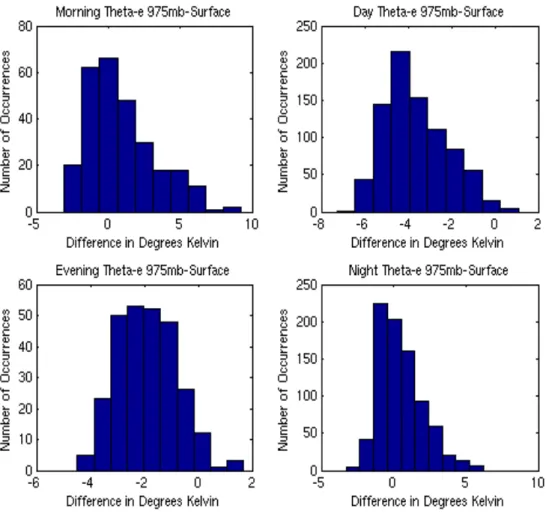
Summer is also characterized by large fluctuations in the diurnal temperature range [Sun et al., 2006]. Therefore, large fluctuations in atmospheric stability will be present in the lower atmospheric levels throughout the diurnal cycle. In addition, boundary layer wind speeds are a strong function of atmospheric stability [Sumner and Masson, 2006]. In order to quantify the diurnal range of wind speeds in the lower levels, vertical profiles of equivalent potential temperature were computed to estimate stability as a function of local standard time (LST) (Figure. 2.2). Based on this analysis, the study period was divided into 4 different categories: (i) daytime unstable (0900-1700 LST), (ii)
evening transition (1800-2000 LST), (iii) nocturnal stable (2100-0500 LST), and finally (iv) morning transition (0600-0800 LST). As seen in figure 2.2, during the day and evening time periods the atmospheric thermodynamic profiles are characterized by mainly unstable conditions due to the strong solar heating at the surface. The evening transition period seems characterized by a gradual transition to a more neutral
16
Figure 2.2 Histogram of the difference in equivalent potential temperature between 975 mb and the surface for Chalmers Township from 06/01/08 – 08/31/08. Top Left: Morning transition regime (6a-8a LST). Top Right: Day convective regime (9a-5p LST). Bottom Left: Evening transition regime (6p-8p LST). Bottom Right: Night stable regime (9p-5a LST). Negative values are inherent of a thermodynamically unstable environment. Positive values characterize a thermodynamically stable environment.
17
state as the emission of surface longwave radiation exceeds the absorption of shortwave radiation. During the nocturnal and early morning periods, strong static stability is seen due to the development of a surface based inversion before transitioning to a more neutral
profile as late morning arrives. 4 different sets of weights corresponding to these 4 stability regimes were calculated.
2.3 WRF-SCM Ensemble
The single-column version of the Weather Research and Forecasting (WRF-SCM) model was used to generate wind speed forecasts at 90m height. WRF-SCM is a 1-dimensional stand-alone implementation of the WRF mesoscale numerical weather prediction model [Skamarock et al., 2005; Hacker et al., 2007]. The WRF-SCM is just like the WRF 3-dimensional model, which also has a wide range of parameterizations for turbulent mixing and closure, radiation,
microphysics and surface fluxes. The options include different sub grid parameterizations for the surface layer and the planetary boundary layer (PBL) that can simulate different stability regimes.
18
The model domain is centered on the location of the
meteorological tower in Chalmers Township, IL. The vertical domain spans from the surface to a height of 12 km and encompasses 120 vertical levels. With 6-7 layers in the lowest 100 m, the model is capable of adequately resolving the lower PBL where the wind speed sensor is located. Since the model forecast wind speeds for pressure levels, the model forecasts are linearly interpolated to 90 m height in order to compare with the tower observations.
The model is initialized with horizontal winds, potential
temperature, moisture, surface pressure, soil temperature, and soil moisture fraction from the hourly-updated 20 km RUC 0-hour forecast data for the RUC model grid cell containing the study site. The RUC 0-hour forecast is essentially a 3-dimensional real-time meteorological analysis dataset that assimilates observations from a wide range of surface, tower and remote sensing instruments. The model is
numerically integrated at 1 s time steps for 1-hour to generate the forecast.
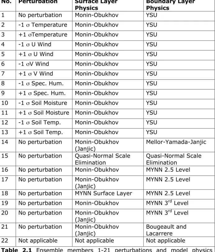
A 22-member ensemble forecast of wind speeds was constructed to predict wind speeds at the Chalmers Township tower location (Table 2.1). The ensemble consists of a baseline run (member 1), 12 initial
19
No. Perturbation Surface Layer
Physics Boundary Layer Physics
1 No perturbation Monin-Obukhov YSU 2 -1 σ Temperature Monin-Obukhov YSU
3 +1 σTemperature Monin-Obukhov YSU
4 -1 σ U Wind Monin-Obukhov YSU
5 +1 σ U Wind Monin-Obukhov YSU
6 -1 σV Wind Monin-Obukhov YSU
7 +1 σ V Wind Monin-Obukhov YSU
8 -1 σ Spec. Hum. Monin-Obukhov YSU
9 +1 σ Spec. Hum. Monin-Obukhov YSU
10 -1 σ Soil Moisture Monin-Obukhov YSU
11 +1 σ Soil Moisture Monin-Obukhov YSU
12 -1 σ Soil Temp. Monin-Obukhov YSU
13 +1 σ Soil Temp. Monin-Obukhov YSU
14 No perturbation Monin-Obukhov
(Janjic) Mellor-Yamada-Janjic 15 No perturbation Quasi-Normal Scale
Elimination Quasi-Normal Scale Elimination 16 No perturbation Monin-Obukhov MYNN 2.5 Level 17 No perturbation Monin-Obukhov
(Janjic) MYNN 2.5 Level
18 No perturbation MYNN Surface Layer MYNN 2.5 Level 19 No perturbation Monin-Obukhov MYNN 3rd Level
20 No perturbation Monin-Obukhov
(Janjic) MYNN 3
rd Level
21 No perturbation Monin-Obukhov
(Janjic) Bougeault and Lacarrere 22 Not applicable Not applicable Not applicable
Table 2.1 Ensemble members 1-21 perturbations and model physics
20
condition perturbation runs (members 2-13), 8 model physics variation runs (members 14-21) and a persistence model (member 22). The baseline case was run with the Monin-Obukov surface layer [Monin and Obukhov, 1954] and the YSU boundary layer physics schemes [YSU; Hong et al. 2006] and initialize it with the RUC model analysis as
described above. The RRTM scheme [Mlawer et al., 1997] for longwave radiation, the Dudhia [Dudhia, 1989] scheme for shortwave radiation and the Unified Noah land-surface model to represent land-surface processes was used for all of the other physics options.
For the perturbation cases the baseline model was run with
perturbation in the initial conditions. The role of the perturbation runs is to incorporate realistic errors in initialization in the ensemble to produce a realistic estimate of uncertainty in the forecasts. [Roquelaure and Bergot, 2007] It has been have shown that forecast uncertainty and errors in initialization are correlated with the intrinsic variability of the initial conditions. Instead of using random perturbations in the initial vertical profiles, perturbations were calculated as the standard deviation of the data estimated from the 3-month long study period. The initial conditions are obtained by adding a perturbation equal to ± 1 standard deviation to the vertical profiles of one of the following parameters: air
21
temperature, air specific humidity, zonal and meridional winds and soil moisture and temperature. For example, if the initial temperature T(k) at the k-th atmospheric level for ensemble member 2 is given by T(k) = T0(k) - σ(k), where T0(k) and σ(k) are the observed unperturbed
temperature and standard deviation of temperature calculated from RUC analysis, respectively.
To account for uncertainties due to model imperfections, a set of 8 model physics runs were conducted using various combinations of 4 surface layer physics schemes and 4 PBL schemes. Compatibility checks were conducted to make sure that the surface layer and PBL schemes are compatible with each other. In addition, a persistence model was implemented for the assumption that that the wind speed remained constant for the simulation period.
The WRF-SCM was chosen in this study due to the
computationally efficiency of 1-dimensional models and accuracy of the WRF-SCM antecedent, the WRF 3-dimensional model. The generation of the WRF-SCM deterministic forecast and calibration by BMA using a sequential LINUX operating system can be completed in less than a minute.
22
Using this configuration a total of 46368 hour-long simulations were conducted. Out of these 30744 are used to calibrate the
ensembles and the remaining 15624 simulations are used to evaluate the forecasts.
2.4 BMA Calibration
The 22 members of the WRF-SCM ensemble system can be considered as independent estimates of wind speeds for a particular time at the given location. However, these estimates may not be equally likely and hence the ensemble needs to be calibrated. The ensemble was calculated using the BMA technique following the
algorithm developed by Raftery et al. (2005). A public-domain code is available at http://cran.r-project.org/web/packages/ensembleBMA.
In BMA, the overall forecast PDF is a weighted average of forecast PDF’s based on each of the individual member’s forecasts. The weights are the estimated posterior model probabilities and reflect the models’ forecast skill in the training period. The BMA deterministic forecast is just a weighted average of the forecasts from the ensemble. The BMA forecast variance decomposes into two components, corresponding to
23
between-model and within-model variance. The ensemble spread captures only for first component. This decomposition provides a theoretical explanation and quantification of the behavior observed in several ensembles, in which a significant spread-skill relationship coexists with a lack of calibration.
To solve the problem of underestimating uncertainty in an
ensemble forecasting system, Bayesian model averaging conditions the ensemble not on a single “best” model but on the entire ensemble of dynamical and/or statistical models (Leamer 1978; Kass and Raftery 1995; Hoeting, Madigan, Raftery, and Volinsky 1999). We represent the quantity to be forecasted as
€
y
. Each ensemble member deterministic forecast,€
f
k, can be corrected, yielding a bias-corrected forecast€
f
k ~ . The forecast€
f
k is then associated with aconditional PDF,
€
g
k(
y
|
f
~k)
, which can be interpreted as the conditional PDF of€
y
conditional on€
f
k ~ , given that€
f
k is the best forecast in theensemble. The BMA predictive model is then,
€
p
(
y
|
f
1,...,f
k)
=
w
kg
k(
y
|
f
~k)
k=1 K
24
€
w
k is the posterior probability of forecast€
k
being the best one, and is based on forecast€
k
’s skill in the training period. The€
w
k’s are weights so they must add up to 1 [Raftery et al., 2005].€
w
k=
1
k=1 K
∑
(2)For simplicity we approximate the wind speed forecast using a normal distribution centered on
€
f
~k, so that€
g
k(
y
|
f
~k)
is a normal PDF with mean€
f
~k and a member specific standard deviation
€
σ
k. Werepresent this situation by,
€
y
|
f
~k~
N
(
f
~ k,
σ
k2
)
(3)The BMA predictive mean is just the conditional expectation of
€
y
given the forecasts, namely€
E[
y
|
f
1,...,
f
k]
=
w
kf
~k k=1K
∑
(4)Equation (4) can now be viewed as a deterministic forecast since it is just the summation of the weighted ensemble-member specific forecast times their individual forecasts. This deterministic forecast can now be
25
compared to other forecasts to measure performance [Raftery et al., 2005].
We now consider how to estimate the model parameters,
€
w
k and€
σ
2, from€
k
=1,..., €K, on the basis of training data. We represent the set
of BMA model parameters to be estimated by
€
θ. We denote space and
time by subscripts s and t, so that
€
f
kst denotes the kth forecast in the ensemble for place s and time t, and€
y
stdenotes the corresponding verification.We estimate
€
θ by maximum likelihood [Fisher, 1922] from the
training data. The likelihood function is defined as the probability of the training data given
€
θ, viewed as a function of
€
θ. The maximum
likelihood estimator is the value of
€
θ that maximized the likelihood
function such as the value of the parameter under which the observed data were most likely to have been observed [Caselia and Berger, 2001].
It is convenient to maximize the logarithm of the likelihood function rather than the likelihood function itself, for reasons of both algebraic simplicity and numerical stability. The log-likelihood function for is
26
€
(
θ
)
=
log(
w
kg
k(
y
st|
f
kst~))
k=1 K∑
s,t∑
(5)where the summations is over values of s and t that index observations in the training set. This cannot be maximized analytically, and it is complex to maximize numerically using direct nonlinear maximization methods such as Newton-Raphson and its variants. Instead, we maximize it using the expectation-maximization, or EM algorithm [Dempster, Laird, and Rubin 1977; McLachlan and Krishman 1997].
The EM algorithm is a method for finding the maximum likelihood estimator when the problem can be recast in terms of “missing data” such that, if we knew the missing data, the estimation problem would be straightforward. The missing data does not have to be actual
missing data. Instead, they are often latent or unobserved quantities, knowledge of which would simplify the estimation problem. The BMA model is a finite mixture model (McLachlan and Peel 2000). Here we introduce “missing data”
€
z
kst where€
z
kst=1 if ensemble member€
k
is the best forecast for verification place s and time t, and€
z
kst=1 otherwise. For each (s, t) only one of {€
z
1st,...,
z
kst} is equal to 1; the others are all zero [Raftery et al., 2005].27
The EM algorithm is iterative, and alternates between two steps, the E (or expectation) step, and the M (or maximization) step. It starts with an initial guess,
€
θ(0), for the parameter vector
€
θ. In the E step, the
€
z
kst are estimated given the current guess for the parameter; the estimates of the€
z
kst are not necessarily integers, even though the true values are 0 or 1. In the M step,€
θ is estimated given the current
values of the
€
z
kst.For the normal BMA model, the E step is
(6)
where the superscript
€
j
refers to the€
j
th iteration of the EM algorithm€
g
(
y
st|
f
~kst,σ
k(j−1)
)
is a normal density with mean€
f
~ kst, and standard deviation€
σ
k (j−1) evaluated at€
y
st. The M step then consists of estimating the€
w
k and the€
σ
k using as weights the current estimates of€
z
kst, i.e.€
ˆ
z
kst(j). Thus€
w
k(j)=
1
n
z
ˆ
kst (j) s,t∑
(7)28
€
σ
k 2(j)=
s,tz
ˆ
kst (j)(
y
st−
f
˜
kst)
2∑
s,tz
ˆ
kst (j)∑
(8)where n is the number of observations.
The E and M steps are iterated to convergence, which we defined as changes no greater than 1e-8 in any of the log-likelihood, the
parameter values, or the
€
ˆ
z
kst(j)
in one iteration. The log-likelihood is guaranteed to increase at each EM iteration (Wu 1983), which implies that in general it converges to a local maximum of the likelihood. How fast this algorithm takes to arrive at a solution is strongly dependent on the initial starting values [Raftery et. al., 2005].
Using data from the 06/01/2008-07/31/2008 period, 4 sets of weights were estimated for each ensemble member corresponding to the 4 different stability regimes discussed earlier. Next, a dynamic training period approach was used where the forecasts for a particular day are calculated from an ensemble that is calibrated with training data from the previous 60 days. Finally, sensitivity simulations were conducted by changing the training period from 2 months to 2 weeks.
In the dynamic training period approach, the calibration weights are constantly updated by incorporating new information and discarding
29
old information. This approach can lead to better forecasts if the wind regime is changing, e.g., if the wind regime during August is
significantly different from that during June-July. A shorter training period that emphasizes latest information can further improve the forecasts in a rapidly changing environment.
2.5 Forecast Quality Control
This study is only valid for non-precipitation time periods at the study location. This was done in order to simplify the problem of weight calibration. Summer time precipitation events are usually convective, which allow for the formation of gust fronts, microbursts, and other mesoscale or microscale features. Since these events have very
different weather characteristics compared to dry and docile conditions they were subsequently removed. Table 2.2 shows the times and dates removed due to precipitation. Precipitation time periods were identified by using Iowa Environmental Mesonet available at:
(http://mesonet.agron.iastate.edu/current/mcview.phtml). If
precipitation occurred at or in close proximity to the study location from June 1st – August 31st those times were discarded from weight
30 2.6 Observation Quality Control
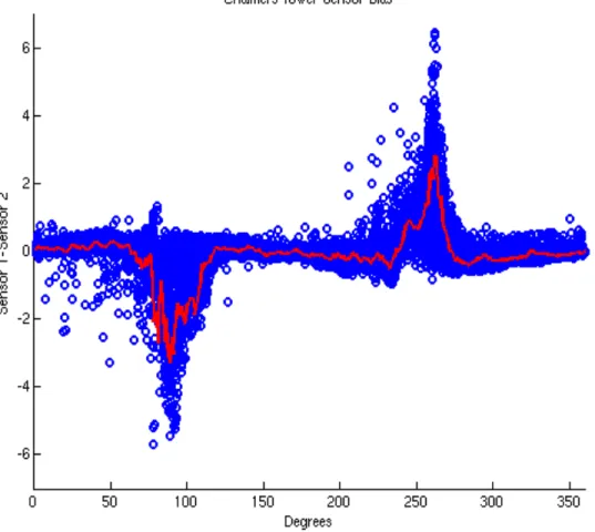
Another source of possible uncertainty in this study stems from the use of imperfect observations from the 90m tower at the site location. At 90m height the tower possessed two sensors, one on the westward face and one on the eastward face of the tower. As you can see from figure 2.3, wind speed measured by the two sensors is a strong function of direction. When the wind originated from 270 degrees (westerly wind) sensor 1 recorded, on average, a larger measurement of around 2.5 m/s. When the wind originated from 90 degrees (easterly wind) sensor 2 recorded a larger average
measurement of around 2.5 m/s. It is believed that the tower caused some distortion in the wind field as the wind propagated by the sensors. In this study, the higher tower sensor observation was used in order to try and eliminate another possible source of uncertainty caused by flow obstruction.
2.7 Forecast Evaluation
Ensemble simulations with the WRF-SCM to forecast 90 m wind speeds at the Chalmers Township tower location for the 08/01/2008 08/31/2008 period were conducted. The linear mean of the forecasts
31
Date Start Time End Time Date Start Time End Time
2-Jun 9:00 AM 11:00 PM 3-Jul 6:00 AM 8:00 AM 3-Jun 12:00 AM 11:00 PM 7-Jul 2:00 AM 4:00 AM 4-Jun 12:00 AM 10:00 AM 8-Jul 1:00 AM 9:00 AM 5-Jun 12:00 AM 9:00 AM 8-Jul 12:00 PM 11:00 PM 6-Jun 12:00 AM 10:00 AM 12-Jul 2:00 PM 7:00 PM 7-Jun 12:00 PM 5:00 PM 18-Jul 7:00 PM 12:00 AM 8-Jun 9:00 PM 11:00 PM 19-Jul 1:00 AM 3:00 AM 9-Jun 12:00 AM 11:00 PM 20-Jul 1:00 AM 3:00 AM 10-Jun 12:00 AM 4:00 AM 21-Jul 4:00 AM 8:00 AM 11-Jun 12:00 AM 2:00 AM 21-Jul 7:00 PM 11:00 PM 12-Jun 1:00 PM 1:00 PM 22-Jul 12:00 AM 12:00 AM 13-Jun 12:00 AM 11:00 PM 24-Jul 3:00 AM 2:00 PM 13-Jun 6:00 PM 7:00 PM 27-Jul 7:00 PM 12:00 AM 15-Jun 2:00 PM 4:00 PM 28-Jul 3:00 AM 6:00 AM 21-Jun 5:00 AM 7:00 AM 29-Jul 5:00 PM 12:00 AM 22-Jun 2:00 PM 4:00 PM 30-Jul 12:00 AM 7:00 AM 24-Jun 1:00 PM 12:00 AM 3-Aug 4:00 AM 11:00 AM 25-Jun 12:00 AM 9:00 AM 5-Aug 6:00 AM 12:00 PM 25-Jun 11:00 PM 11:00 PM 5-Aug 5:00 PM 7:00 PM 26-Jun 12:00 AM 8:00 AM 12-Aug 6:00 PM 7:00 PM 27-Jun 4:00 AM 2:00 PM 14-Aug 4:00 PM 7:00 PM 28-Jun 2:00 AM 4:00 AM 20-Aug 9:00 PM 12:00 AM 28-Jun 3:00 PM 4:00 PM 21-Aug 12:00 AM 2:00 PM 2-Jul 7:00 AM 9:00 AM 28-Aug 8:00 AM 12:00 PM 2-Jul 5:00 PM 11:00 PM 28-Aug 7:00 PM 11:00 PM Table 2.2 Precipitating time periods that were eliminated from the weight calibration and verification.
32
from individual ensemble members constitutes the uncalibrated ensemble forecast. The calibrated ensemble was calculated with the BMA-calibrated ensemble forecasts using the weights estimated from the training simulations. The performance of the uncalibrated and calibrated ensemble forecasts were evaluated by comparing them with observations and computing 3 statistics: mean absolute error (MAE) root mean square error (RMSE) and Bias The statistical significance of the performance improvements are estimated using the Students’ t test. Only results valid at 80% or higher levels will be considered statistically significant
€
MAE
=
1
n
i=1|
F
i−
O
i|
n∑
(9)€
RMSE
=
1
n
(
F
i−
O
i)
2 i=1 n∑
(10)€
BIAS
=
1
n
i=1(
F
i−
O
i)
n∑
(11)33
Figure 2.3 Tower wind observations during the study period. The blue dots represent sensor bias from 0° to 359°. The red line represents a 5-degree moving average centered on the wind direction angle.
34 3. RESULTS
3.1 Example Forecast
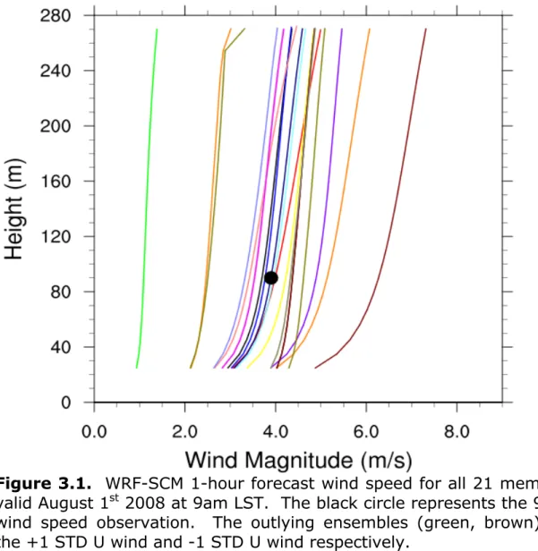
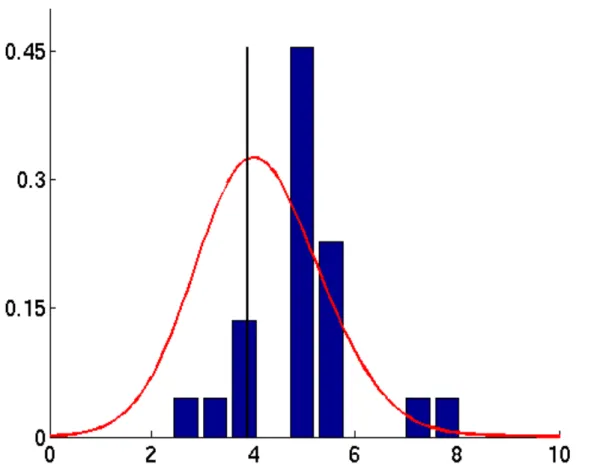
Since it is impossible to plot the results of all 46368 simulations, an example the vertical profiles of wind speed forecasts from all models for 9 am LST on 08/01/2008 is shown in Figure 3.1. All the simulated profiles are qualitatively similar, with wind speed decreasing with height, and distributed around the observed value at 90m height. The corresponding PDF from the BMA-calibrated ensembles for the same period is more evenly distributed around the observed value that the uncalibrated ensemble PDF (Figure 3.2). The BMA-calibrated ensemble PDF is essentially the weighted sum of the individual ensemble
member’s PDF. Thus simple visual inspection indicates that BMA calibration improves ensemble predictability for this case.
3.2 Calibrated vs. Uncalibrated Ensemble
For a comprehensive evaluation of the performance of the calibrated ensemble forecast error statistics for the entire month of August 2008 were calculated (Table 3.1). The statistics show that the calibrated ensemble forecasts convincingly outperform the uncalibrated
35
Regime Forecast Method RMSE MAE Bias
Uncalibrated 3.384 2.8855 -2.7979 Calibrated 1.1456 0.8655 0.2405 Morning Transition 0600-0800 LST Persistence 1.255 0.9559 0.5188 Uncalibrated 1.1307 0.8978 -0.4645 Calibrated 0.9249 0.7192 -0.0821 Unstable 0900-1700 LST Persistence 1.0348 0.7884 0.0232 Uncalibrated 2.7015 2.2088 -2.0755 Calibrated 1.1478 0.9479 -0.4735 Afternoon Transition 1800-2000 LST Persistence 1.0809 0.9042 -0.2664 Uncalibrated 4.4229 4.0831 -4.0698 Calibrated 1.2328 0.8668 -0.1 Stable 2100-0500 LST Persistence 1.2391 0.8691 -0.0723 Table 3.1 Score statistics for the 60-day fixed window for each time/stability regime
36
Figure 3.1. WRF-SCM 1-hour forecast wind speed for all 21 members valid August 1st 2008 at 9am LST. The black circle represents the 90 m
wind speed observation. The outlying ensembles (green, brown) are the +1 STD U wind and -1 STD U wind respectively.
37
Figure 3.2. Probability density function of the uncalibrated (blue bars) and calibrated (red line) ensemble forecast for 08/01/2008 at 9a LST. The grey vertical line denotes the value of the observation
38
ensemble forecasts in all 4 regimes. Calibration significantly reduces forecast errors in all three error measures by 20%-100% with bias being the greatest improvement. Maximum percentage improvements are observed during the nocturnal stability regime while the diurnal convective regime shows the least improvement. This is due to the change in the weight, and subsequent performance, of persistence will be described in detail in a later section. All these improvements are statistically significant at 99% or higher level of significance using the Student’s T-Test.
3.3 RUC Model Bias Effects
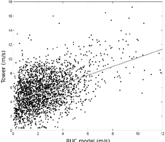
Amongst the 3 error measures, the BMA calibration produces the strongest improvement in bias. It is clear from the results that the uncalibrated forecast significantly and consistently under predicts wind-speed. The likely reason behind this phenomenon is the initial
conditions obtained from the RUC model have a strong negative bias in wind speed compared to the tower observations (Figure 3.3).
The negative bias in the initial conditions during the morning, day, evening and night regimes are -4.18 m/s, -2.85 m/s, -1.43 m/s and -3.51 m/s respectively. These biases are all statistically significant at higher than the 99.99% level of significance.
39
Figure 3.3. Scatter plot of the wind speed measured by the sensor at 90 m height on the Chalmers township tower and the wind speed interpolated to 90 m height from the RUC model 0-hour analyses. The grey line is the linear fit between the 2 datasets.
40
3.4 Calibrated Ensemble Member Performance
The weights given to the different ensemble members can be very different and can range several orders of magnitude. The weights from the ensemble calibration (Table 3.2) can be used as a quantitative measure of the performance of each ensemble member. It is clearly evident that the persistence model consistently outperforms the numerical models in all 4 stability regimes. Amongst the numerical models, members 2, 4, 5, and 7 provide meaningful results with some degree of consistency. These ensemble members all reside in the initial condition perturbation group with members 5 and 7 representing +1σ U and V wind perturbations.
3.5 Convective Daytime Regime
The numerical models perform the best during the diurnal
unstable regime. Even though the persistence model performs better, its assigned weight during this period is 66%. This implies that with a combined weight of 34%, the numerical models make a significant contribution to the calibrated ensemble forecasts. Strong convection during the summer leads to high-frequency turbulent variability in wind speeds during the daytime. The persistence model by itself cannot adequately capture this variability. The numerical models perform
41
reasonably well in simulating the daytime convective boundary layer. Due to strong contribution from the numerical models, the calibrated ensemble forecasts show and 11% improvement in RMSE over the persistence model statistically significant at the 85% level (Table 3.1). This result implies that a calibrated ensemble approach that blends persistence and numerical models is the best approach in generating hourly wind speed forecasts in unstable convective environments.
3.6 Stable Nocturnal and Transition Regimes
The calibrated ensemble does not produce any statistically significant improvement over the persistence model in the nocturnal and transition regimes. The aggregated weights of the numerical models are quiet low, ranging between 1-13% during these regimes (Table 3.2). The relatively poor performance of numerical models like WRF in nocturnal stable regimes is not unusual and has been reported by other studies [Draxl et al., 2010; Shin and Hong, 2011]. Improving numerical models will be the key to improving the performance of the calibrated ensemble forecasts in stable and transition environments.
42
Weights from BMA calibration Ensemble No. Morning Transition 0600-0800 LST Unstable 0900-1700 LST Afternoon Transition 1800-2000 LST Stable 2100-0500 LST
1 2.34E-11 9.46E-05 7.27E-08 1.21E-68
2 4.75E-06 0.04546314 0.02034182 1.32E-63 3 1.06E-10 0.2033106 2.55E-06 5.78E-58 4 0.02711173 0.02630156 4.09E-16 7.57E-21 5 0.03361364 0.009373185 7.48E-35 0.000187818
6 2.62E-09 1.02E-83 4.10E-91 1.70E-27
7 0.0654014 0.05530994 3.77E-45 0.01248482
8 1.50E-10 1.22E-07 1.12E-05 1.99E-68
9 1.05E-08 0.001934105 7.95E-04 8.33E-54 10 8.62E-11 0.00017959 9.83E-10 9.74E-69 11 9.85E-12 6.43E-05 1.26E-05 1.26E-68 12 2.76E-10 6.66E-05 2.82E-06 9.38E-68 13 2.97E-09 0.000158572 5.57E-13 1.24E-66 14 1.13E-17 2.12E-16 5.36E-02 1.29E-27 15 8.85E-20 2.12E-30 7.85E-23 1.26E-29 16 4.99E-20 8.40E-53 1.37E-19 1.82E-24 17 1.32E-23 3.98E-81 4.43E-19 2.39E-23 18 2.61E-16 4.37E-27 2.04E-10 3.47E-24 19 4.99E-20 8.40E-53 1.37E-19 1.82E-24 20 1.32E-23 3.98E-81 4.43E-19 2.39E-23 21 2.97E-18 1.25E-82 0.01544482 9.23E-65 22 0.8738686 0.6578446 0.9042015 0.9873274
Table 3.2 Ensemble member weights for the 60-day fixed window for
43 3.7 Training Window Sensitivity
The results discussed so far are based on ensembles calibrated using observations from June 1 – July 31 2008 and evaluated against observations from August 2008. I studied the importance of training on the calibrated forecasts by using the following 3 other training periods:
i. 2-week training period
ii. 2-month moving training period and iii. 2-week moving training period.
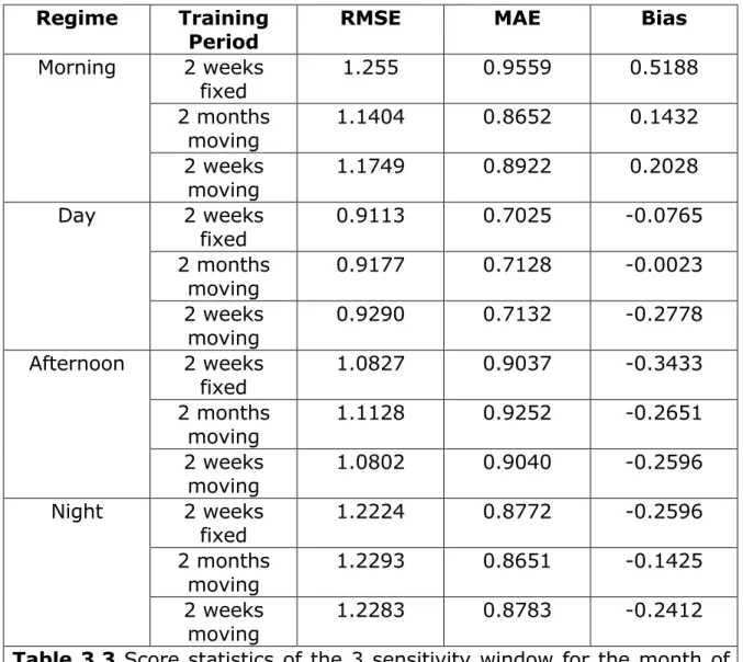
The results of the sensitivity studies are shown in Table 3.3. In the first sensitivity study, the ensembles are calibrated using a 2-week period (July 17-July 31) instead of the 2-month training period used above. Using a shorter training period significantly degrades the
forecast bias during the morning transition and nocturnal stable regime. However, this improvement is small (~0.01 m/s) and the statistical significance is primarily due to a change in sign of the bias error from negative in the 2-month training period study to positive in the 2-week training period. Differences in other error measures are small and not statistically significant.
The final 2 sensitivity studies involve moving training periods where each forecast is calibrated with a unique dataset. For example, in the second sensitivity study, the ensemble forecast for each day is
44
Regime Training
Period RMSE MAE Bias
2 weeks fixed 1.255 0.9559 0.5188 2 months moving 1.1404 0.8652 0.1432 Morning 2 weeks moving 1.1749 0.8922 0.2028 2 weeks fixed 0.9113 0.7025 -0.0765 2 months moving 0.9177 0.7128 -0.0023 Day 2 weeks moving 0.9290 0.7132 -0.2778 2 weeks fixed 1.0827 0.9037 -0.3433 2 months moving 1.1128 0.9252 -0.2651 Afternoon 2 weeks moving 1.0802 0.9040 -0.2596 2 weeks fixed 1.2224 0.8772 -0.2596 2 months moving 1.2293 0.8651 -0.1425 Night 2 weeks moving 1.2283 0.8783 -0.2412
Table 3.3 Score statistics of the 3 sensitivity window for the month of August 2008 broken down by time/stability regime.
45
calibrated with data from the previous 60 days. Similarly, the third sensitivity study uses data from the previous 2 weeks to calibrate each day’s forecast. Results of these sensitivity studies (Table 3.3) show that the 60-day moving period generates and improved forecast and the 2-week moving training period generates a degraded forecast when compared with the 60-day fixed training period. However, these
changes are small in magnitude and statistically insignificant except the degradation in forecast with the 2-week moving training period during the nocturnal stable regime.
46 4. CONCLUSIONS AND DISCUSSIONS
In this work a computationally efficient and accurate method to provide wind speed forecasts over 1-hour timescales for wind energy applications is developed. For this purpose I used an adaptive blended statistical-dynamical ensemble forecast system that is calibrated with and evaluated against data from a potential wind farm site. This system provides significantly more accurate forecasts than the uncalibrated ensemble for all stability environments and better
forecasts than the persistence model during daytime convective stability regimes. In particular, the BMA calibration method largely eliminates the strong negative bias in the forecasts due to the negative bias in the model initialization.
This approach is computationally much more efficient compared to traditional mesoscale NWP models. NWP models require enormous computing resources, especially for conducting ensemble simulations. In contrast, this system can generate a calibrated ensemble forecast in less than 1 minute on a single processor LINUX PC. Hence, this
forecast system can easily be adopted by small wind farm owner/operators with limited financial resources.
This study demonstrates that there is a strong need for improving the capabilities of numerical models to simulate the stable boundary
47
layer and the stable-unstable transition periods. Until numerical models improve significantly, persistence will continue to be the method of choice for forecasting nocturnal wind speeds. It needs to be pointed out that persistence is far from a perfect solution because forecast errors are quite high. However, an ensemble of persistence and
improved numerical model forecasts calibrated with the BMA technique can potentially reduce the forecast errors.
Sensitivity studies with different training periods to calibrate different ensembles did not produce conclusive results. The goal of the training is to assign weights depending on the performance of each model under a wide range of meteorological conditions. A very short training period will not be able to capture the range of natural variability in wind speeds and hence will lead to poor quality forecasts. The
results suggest that a week training period may be too short and a 2-month training period is probably required to produce quality forecasts. Figure 4.1 cast further light that there exists a 18 day cycle of wind speeds which would not be adequately captured by the 2 week training window. In addition, a 31-day cycle is also present which may suggest that the 2-month window may be too long of a training window.
Moving training periods that emphasize new information at the expense of old information are expected to produce better forecasts if the
48
Figure 4.1 Power spectra of wind speeds during the study period. As you can see there is evidence of a diurnal cycle in wind speed as well as another cycle of around 18 days. In addition, there is also evidence of a planetary scale influence on wind speeds of around 31 days. It is not known what atmospheric phenomena applies to the 3.5-6 days wind speed cycle but frequent occurrences of Mesoscale Convective Systems in the vicinity of the study site were common during this study period.
49
meteorological regimes are changing. In this study, I did not find any statistically significant evidence of this phenomenon. The impact of a moving training period can be adequately tested only if the
meteorological conditions during the training period and forecast period are radically different. I speculate that if the forecast training period were extended by many months, the benefit of using a moving versus a fixed training period would become more readily apparent.
Overall, this study demonstrates that BMA calibration of ensemble forecasts of wind speeds can significantly improve forecast quality. More work is required to find the most appropriate training periods that will provide the maximum improvement over uncalibrated forecasts.
50 5. FUTURE WORK
It is evident that Bayesian Model Averaging is a powerful
statistical technique for calibrating ensemble prediction models. With the projected rapid future growth of the wind power industry,
ensemble-forecasting techniques will be essential in the reduction of cost and financial risks associated with the difficulty of wind prediction.
Future work might explore the effectiveness of the calibrated ensemble system at forecasting for other time periods. Calibration for transition seasons such as spring and fall may rely heavily on a moving window since the synoptic weather regime at the beginning of the season may be drastically different from the end. In this case, it is quite likely that the performance of the individual ensemble members will change drastically throughout the study period. Cold season
forecasting should also be explored. It would be interesting to see how the NWP models handle the semi-permanent presence of a surface inversion.
Exploring different training window lengths should also be researched. In this study, a 2-week and two month training window was implemented. In figure 4.1 there was a strong power peak at 31-days. Therefore, a 1-month training window may be the optimal window length.
51
In addition, different study site locations may also be explored to see if the forecasting system is also geographically robust.
Implementation of this forecasting system in other highly desirable wind power locations will be needed.
Better understanding the degree to which BMA reduces the level of uncertainty in the forecast should also be explored. If the standard deviation of the calibrated with respect to the uncalibrated probability distribution function decreases then calibration reduces uncertainty in the forecast. This is will be extremely valuable for operators who need a range of possible scenarios to help with the decision process for their business.
Wind power operators also need accurate forecasts of high wind events to prevent damage to their equipment. Preliminary work has shown that the BMA calibrated ensemble is able to capture some of the ramp events that the uncalibrated ensemble cannot. More work is needed to better understand how well BMA can capture the probability of high wind events to protect wind farm operators from unnecessary equipment damage.
52 6. REFERENCES
Bougeault, P. and P. Lacarrere, 1989. Parameterization of orography-induced turbulence in a mesobeta-scale model, Mon. Wea. Rev., 117, 1872-1890.
Buizza, R., Miller M, and Palmer, T. N., 1999. Stochastic representation of model uncertainties in the ECMWF Ensemble Prediction System. Quart. J. Royal Meteorol. Soc., 2887-2908.
Buizza, R., et al., 2005. A comparison of the ECMWF, MSC, and NCEP global ensemble prediction systems. Mon. Wea. Rev., 133, 1076-1097. Casella, G., Berger R.L., 2001., Statistical inference (2nd ed.). Brooks
Cole.
Costa, A., Crespo, A., Navarro, J., Lizcano, G., Madsen, H. and Feitosa, E., 2008. A review on the young history of the wind power short-term prediction. Renewable Sustainable Energy Revs. 12, 1725-1744. Dempster, A. P., Laird, N. M., and Rubin, D. B., 1977. Maximum likelihood from incomplete data via the EM algorithm. J. Roy. Stat. Soc., 39B, 1–38.
Draxl, C. et al., 2010. Validation of boundary-layer winds from WRF mesoscale forecasts with applications to wind energy forecasting, 19th Symposium on Boundary Layers and Turbulence, American
Meteorological Society, Keystone, CO.
Dudhia, J., 1989. Numerical study of convection observed during the winter monsoon experiment using a mesoscale two-dimensional model. J. Atmos. Sci., 46, 3077-3107.
Duran, M. J., Cros, D. and Riquelme, J., 2007. Short-term wind power forecast based on ARX models. J. Energy Eng. 133, 172-180.
Fisher, R. A., 1992. On the mathematical foundations of theoretical statistics. Philo. Trans. Roy. Soc., 222A, 309-368.
Georgilakis, P. S., 2008. Technical challenges associated with the integration of wind power into power systems. Renewable Sustainable Energy Rev. 2, 852-863.
53
Hacker J. P., Anderson J. L. and Pagowski M., 2007. Improved vertical covariance estimates for ensemble-filter assimilation of near-surface observations. Mon. Wea. Rev., 135, 1021-1036.
Hoeting, J. A., Madigan, D. M., Raftery, A. E., Volinsky, C. T., 1999. Bayesian model averaging: A tutorial (with discussion). Statistical Science 14. 382-401. A corrected version with typos corrected is available
www.stat.washington.edu/www/research/online/hoeting1999.pdf. Hong S. Y. and S. W. Kim, 2008. Stable boundary layer mixing in a vertical diffusion scheme. Proc. 9th annual WRF User’s Workshop, National Center for Atmospheric Research, Boulder CO.
Hong S. Y., Lim J. O., 2006. The WRF single-moment 6-class
microphysics scheme (WSM6). J. Korean Meteor. Soc., 42, 129-151 Janjic, 1994. The step-mountain Eta-coordinate model: Further
developments of the convection, viscous sublayer and turbulent closure schemes, Mon. Weather Rev., 122, 927-945.
Janjic, Z. I., 2001. Nonsingular implementation of the Mellor-Yamada level 2.5 scheme in the NCEP meso model, NOAA/NWS/NCEP Office Note 437, 61 pp, Available online at
www.emc.ncep.noaa.gov/officenotes/newernotes/on437.pdf. Kass, R.E. and Raftery, A. E., 1995. Bayes factors. Journal of the American Statistical Association 90, 773-795.
Leamer, E. E., 1978. Specification Searches. Wiley.
Lei, M., Shiyan, L., Chuanwen, J., Hongling, L. and Yan, Z., 2009. A review on the forecasting of wind speed and generated power. Renewable Sustainable Energy Rev., 13, 915-920.
Lew et al., 2010, “How do Wind and Solar Power Affect Grid
Operations: The Western Wind and Solar Integration Study,” in Proc. 8th International Workshop on Large Scale Integration of Wind Power and on Transmission Networks for Offshore Wind Farms, to appear.
54
McCabe, G. J. et al., 2001. Trends in the northern hemisphere surface cyclone frequency and intensity. Journal of Climate, 14, 2763-2768. Min, K.D. and Horn, H. L., 1992. Available potential energy in the northern hemisphere during the FGGE year. Tellus, 34, 526-539. MacLachlan, G. J., and Krishnan, T., 1997. The EM Algorithm and Extensions. John Wiley and Sons, 274.
McLachlan, G. J., and Peel, D., 2000. Finite Mixture Models. Wiley. McSharry, P. E.; Bouwman, S.; Bloemhof, G., 2005. Probabilistic
forecasts of the magnitude and timing of peak electricity demand. IEEE Trans. Power Systems, 20, 1166 – 1172.
Mlawer, E. J., Taubman, S. J., Brown, P. D., and Iacono, M. J., 1997. Radiative transfer for inhomogeneous atmospheres: RRTM, a validated correlated-k model for the longwave. J. Geophy. Res., 102, 16 663-16 682.
Molteni, F. et al., 1996. The ECMWF ensemble prediction system: Methodology and validation. Quart. J. Royal Meteorol. Soc., 122, 73-119.
Monin, A. S. and A. M. Obukhov, 1954. Basic laws of turbulent mixing in the surface layer of the atmosphere. Contrib. Geophys. Inst. Acad. Sci. USSR, 151, 163-187.
Nakanishi, M. and H. Niino, 2004. Development of an improved turbulence closure model for the atmospheric boundary layer, J. Meteorol. Soc. Japan, 87, 895-912.
NARUC, National Association of Regulatory Utility Commissioners (NARUC), National Wind Coordinating Collaborative (NWCC), and the Western Governors’ Association. 2007. FERC Order 890: What Does It Mean For the West? Available online at
http://www.nationalwind.org/assets/publications/ferc890.pdf.
Palmer, T. N., 2000. Predicting uncertainty in forecasts of weather and climate. Rep. Progress Physics, 63, 71-116.
55
Potter, C et al., 2004. Short-term wind forecasting techniques for power generation. Australasian Universities Power Engineering Conference, 26-29. September 2004, Brisbane, Australia.
Raftery, A.E., Gneiting, T., Balabdaoui, F. and Polakowski, M., 2005. Using Bayesian Model Averaging to Calibrate Forecast Ensembles. Mon. Wea. Rev., 133, 1160-1174.
Riahy, G. H. and Abedi, M., 2008. Short term wind speed forecasting for wind turbine applications using linear prediction method.
Renewable Energy. 33, 35-41.
Roquelaure, S. and Bergot, T., 2008. A local ensemble prediction for fog and low clouds: Construction, Bayesian Model Averaging
calibration and Validation. J. Appl. Meteorol. Climatol., 47, 3072-3088. Sfetsos, A., 2000. A comparison of various forecasting techniques
applied to mean hourly wind speed time series. Renewable Energy, 21, 23-35.
Shin, H. H. and S-Y. Hong, 2011. Intercomparison of Planetary
Boundary Layer parameterizations in the WRF model for a single day from CASES-99, Boundary Layer Meteorol., DOI: 10.1007/s10546-010-9583-z.
Skamarock, W. C., Klemp, J. B., Dudhia, J., Gill, D. O., Barker, D. M., Wang, W. and Powers, J. D., 2005. A description of the Advanced Research WRF version 2.Technical report, National Center for Atmospheric Research, TN-468+STR.
Smith, J. C., DeMeo, E. A., Parsons, B., Milligan, M., 2004. Wind power impacts on electric power system operating costs: summary and
perspective on work to date. NREL, pp 13. Report available online at http://www.nrel.gov/docs/fy04osti/35946.pdf
Sumner, J. and Masson, C., 2006. Influence of atmospheric stability on wind turbine power performance curves. J. Solar Energy Engg. 128, 531-538.
Taylor, J. W., 2004. Forecasting weather variable densities for weather derivatives and energy prices in Modeling Prices in Competitive
56
Electricity Markets, D.W. Bunn, Ed. Chichester, U.K.: Wiley, pp. 307– 330.
Taylor, J. W. and Buizza, R., 2006. Density forecasting for weather derivative pricing. Int. J. Forecasting, 22, 29–42.
Taylor, J. E., McSharry, P. E. and Buizza, R. 2009. Wind power density forecasting using ensemble predictions and time series models. IEEE Trans. Power Systems, 24, 775-782.
Toth, Z. and Kalnay, E., 1997. Ensemble forecasting at NCEP and the breeding method. Mon. Wea. Rev. 125, 3297-3319.
Wu, C. F. J., 1983. On the convergence properties of the EM algorithm. Annals of Statistics 11, 95-103.
United States Department of Energy (DOE) 2008. 20% Wind Energy by 2030. 248 pp. Report available online at
http://www.20percentwind.org/20percent_wind_energy_report_revOct 08.pdf