A New Dantzig-Wolfe Reformulation And Branch-And-Price Algorithm For The Capacitated Lot Sizing Problem With Set Up Times

A New Dantzig-Wolfe Reformulation And

Branch-And-Price Algorithm For The Capacitated Lot Sizing Problem

With Set Up Times

Zeger Degraeve, Raf Jans

ERIM REPORT SERIES RESEARCH IN MANAGEMENT

ERIM Report Series reference number ERS-2003-010-LIS

Publication February 2003

Number of pages 37

Email address corresponding author [email protected]

Address Erasmus Research Institute of Management (ERIM)

Rotterdam School of Management / Faculteit Bedrijfskunde Rotterdam School of Economics / Faculteit Economische Wetenschappen

Erasmus Universiteit Rotterdam P.O. Box 1738

3000 DR Rotterdam, The Netherlands Phone: +31 10 408 1182 Fax: +31 10 408 9640 Email: [email protected] Internet: www.erim.eur.nl

Bibliographic data and classifications of all the ERIM reports are also available on the ERIM website: www.erim.eur.nl

ERASMUS RESEARCH INSTITUTE OF MANAGEMENT

REPORT SERIES

RESEARCH IN MANAGEMENT

B

Abstract The textbook Dantzig-Wolfe decomposition for the Capacitated Lot Sizing Problem (CLSP), as already proposed by Manne in 1958, has an important structural deficiency. Imposing integrality constraints on the variables in the full blown master will not necessarily give the optimal IP solution as only production plans which satisfy the Wagner-Whitin condition can be selected. It is well known that the optimal solution to a capacitated lot sizing problem will not necessarily have this Wagner-Whitin property. The columns of the traditional

decomposition model include both the integer set up and continuous production quantity decisions. Choosing a specific set up schedule implies also taking the associated Wagner- Whitin production quantities. We propose the correct Dantzig-Wolfe decomposition

reformulation separating the set up and production decisions. This formulation gives the same lower bound as Manne’s reformulation and allows for branch-and-price. We use the

Capacitated Lot Sizing Problem with Set Up Times to illustrate our approach. Computational experiments are presented on data sets available from the literature. Column generation is speeded up by a combination of simplex and subgradient optimization for finding the dual prices. The results show that branch-and-price is computationally tractable and competitive with other approaches. Finally, we briefly discuss how this new Dantzig-Wolfe reformulation can be generalized to other mixed integer programming problems, whereas in the literature, branch-and-price algorithms are almost exclusively developed for pure integer programming problems. 5001-6182 Business 5201-5982 Business Science Library of Congress Classification (LCC) _{QA 1-939 Mathematics}

M Business Administration and Business Economics M 11 R 4 Production Management Transportation Systems Journal of Economic Literature (JEL) C 61 Programming models 85 A Business General 260 K 240 B Logistics

Information Systems Management European Business Schools

Library Group (EBSLG)

250 A Mathematics

Gemeenschappelijke Onderwerpsontsluiting (GOO)

85.00 Bedrijfskunde, Organisatiekunde: algemeen 85.34

85.20

Logistiek management

Bestuurlijke informatie, informatieverzorging Classification GOO

31.80 Toepassingen van de wiskunde Bedrijfskunde / Bedrijfseconomie

Bedrijfsprocessen, logistiek, management informatiesystemen Keywords GOO

Series, Integer programming, algoritmen

Free keywords Lot Sizing, Dantzig-Wolfe Decomposition, Branch-and-Price, Lagrange Relaxation, Mixed-Integer Programming

A NEW DANTZIG-WOLFE REFORMULATION AND BRANCH-AND-PRICE ALGORITHM

FOR THE CAPACITATED LOT SIZING PROBLEM WITH SET UP TIMES

Zeger Degraeve London Business School

Regent’s Park, London NW1 4SA, UK Email: [email protected]

Raf Jans*

Rotterdam School of Management, Erasmus University PO Box 1738, 3000 DR Rotterdam, The Netherlands

Email: [email protected]

_____________________________________________________________________

Abstract

The textbook Dantzig-Wolfe decomposition for the Capacitated Lot Sizing Problem (CLSP), as already proposed by Manne in 1958, has an important structural deficiency. Imposing integrality constraints on the variables in the full blown master will not necessarily give the optimal IP solution as only production plans which satisfy the Wagner-Whitin condition can be selected. It is well known that the optimal solution to a capacitated lot sizing problem will not necessarily have this Wagner-Whitin property. The columns of the traditional decomposition model include both the integer set up and continuous production quantity decisions. Choosing a specific set up schedule implies also taking the associated Wagner-Whitin production quantities. We propose the correct Dantzig-Wolfe decomposition reformulation separating the set up and production decisions. This formulation gives the same lower bound as Manne’s reformulation and allows for branch-and-price. We use the Capacitated Lot Sizing Problem with Set Up Times to illustrate our approach. Computational experiments are presented on data sets available from the literature. Column generation is speeded up by a combination of simplex and subgradient optimization for finding the dual prices. The results show that branch-and-price is computationally tractable and competitive with other approaches. Finally, we briefly discuss how this new Dantzig-Wolfe reformulation can be generalized to other mixed integer programming problems, whereas in the literature, branch-and-price algorithms are almost exclusively developed for pure integer programming problems.

1. Problem description

We consider an extension of the basic dynamic lot sizing problem. The planning horizon is split up in discrete time periods and the dema nd for several items over this planning horizon is given. All the items use the same production facility which has a limited capacity in each period. Before an item can be produced in any period, a set up must be performed and the set up time decreases the available capacity. The problem is to find a production plan for all the items that satisfies demand, does not exceed the capacity limit and minimizes the sum of the set up, production and inventory holding costs. This problem is known as the Capacitated Lot Sizing Problem with Set Up Times (CLST). Define the following sets, parameters and variables:

Sets:

P : _{set of products, = {1,…,n},}

T : _{set of time periods, = {1,…,m}.} Parameters:

it

d : demand of product i in period t, ∀ i ∈ P, ∀ t ∈ T itk

sd : sum of demand of product i, from period t until period k,

∀ i ∈ P, ∀ t,k ∈ T : k ≥ t

it

hc : holding cost for product i in period t, ∀ i ∈ P, ∀ t ∈ T it

sc : set up cost for product i in period t, ∀ i ∈ P, ∀ t ∈ T it

vc : variable production cost for product i in period t, ∀ i ∈ P, ∀ t ∈ T fci : unit cost for initial inventory for product i, ∀ i ∈ P

it

st : set up time for product i in period t, ∀ i ∈ P, ∀ t ∈ T

it

vt : variable production time for product i in period t, ∀ i ∈ P, ∀ t ∈ T t

cap : capacity in period t. ∀ t ∈ T

Decision variables: it

x : production of product i in period t, ∀ i ∈ P, ∀ t ∈ T it

y = 1 if set up for product i in period t, = 0 otherwise, ∀ i ∈ P, ∀ t ∈ T sii : amount of initial inventory for item i. ∀ i ∈ P

Min

∑

∑∑

(

)

{

}

(

)

∑

The objective function (1) minimizes the total costs, consisting of the set up cost, the variable production cost, the inventory holding cost and initial inventory cost. Constraints (2.1) and (2.2) are the demand constraints: inventory carried over from the previous period and production in the current period can be used to satisfy current demand and build up inventory. To deal with infeasible problems, we allow initial inventory which is available in the first period at a large feasibility cost of fci (Vanderbeck 1998). There is no set up required for

initial inventory. Constraint (3) forces the set up variable to one if any production takes place in that period. In order to make the formulation stronger, we limit the production for each item by both the remaining demand and the maximum possible production with the available capacity minus the set up time. Next, there is a constraint on the available capacity in each period (4). If we have a set up, the set up time is accounted for. Finally, we have the non-negativity and integrality constraints (5). Let v_CLST be the optimal objective value for problem (1)-(5) and v_CLST its LP relaxation.

This paper is structured as follows. In Section 2, we give a brief literature review on capacitated lot sizing. Section 3 discusses in more detail the traditional Dantzig-Wolfe decomposition for CLST and the structural deficiency of Manne’s formulation. In Section 4, we present the correct Dantzig-Wolfe decomposition reformulation. The different building blocks of the algorithm are described in Section 5. Section 6 presents computational results on data sets available from the literature. Before giving some concluding remarks, we also show in Section 7 how our approach can be extended to other Mixed Integer Programming (MIP) problems.

2. Literature review

The research into dynamic lot sizing models started in 1958 with the seminal paper of Wagner and Whitin. They consider the single item uncapacitated lot sizing model and prove that there exists an optimal solution that satisfies the following property: s_t−1x_t =0, ∀t∈T . This means that in that optimal solution there will never be simultaneous production and inventory carry-over from the previous period. This is called the Wagner-Whitin (WW) property. It also implies that one produces to satisfy the demand for an integer number of consecutive periods. Based on these special properties of the optimal solution, Wagner and Whitin formulate a dynamic programming recursion for solving this problem.

The regular CLST formulation, given by the model (1)-(5), usually has a large integrality gap. Much research is devoted to finding better formulations with a smaller gap. The model can be extended with valid inequalities for the single item uncapacitated lot sizing problem (Barany et al. 1984), which are generally known as the (l, S) inequalities. Adding these cutting planes leads to a formulation which describes the convex hull for the single item uncapacitated lot sizing polytope. Pochet (1988), Leung, Magnanti and Vachani (1989) and Miller, Nemhauser and Savelsbergh (2000) derive several other valid inequalities for the capacitated problem. Belvaux and Wolsey (2000, 2001) report on an efficient branch-and-cut system that includes preprocessing and inequalities for a variety of lot sizing problems. Eppen and Martin (1987) propose another approach for tightening the formulation by using variable redefinition. For the single item uncapacitated problem, this is actually the network formulation of the dynamic programming recursion proposed by Wagner and Whitin (1958) and it gives an integer solution. This network formulation can also be used to tighten more complex problems such as the CLST. Manne (1958) proposes an innovative linear programming formulation for the capacitated multi-item lot sizing problem. He explicitly models all the possible schedules with different set up sequences. For a problem with a planning horizon of m periods, there are 2m different set up schedules for each product, because for each period we either have a set up or not. Manne only considers ‘dominant’ schedules, which have the property that for each period demand will be met by production in that period if there is a set up or otherwise from the nearest preceding period with a set up. Dzielinski and Gomory (1965) explicitly describe the link between Manne’s formulation and the Wagner-Whitin problem. They propose to use column generation to deal with the difficulty of the huge amount of variables in Manne’s formulation. Indeed, the model that Manne proposes is the full blown master for the

Dantzig-problem. Hence, Manne’s dominant schedules are in fact all the Wagner-Whitin schedules. Kleindorfer and Newson (1975) discuss the Lagrange relaxation for the capacitated lot sizing problem. The capacity constraint is now dualized and the problem decomposes into subproblems per item. This lower bound will theoretically be the same as the bound obtained by Dantzig-Wolfe decomposition (Geoffrion 1974). Thizy and Van Wassenhove (1985) implement a Lagrange based heuristic for the capacitated problem. Dual prices are updated by the subgradient method. Trigeiro et al. (1989) also use Lagrange relaxation to solve the capacitated lot sizing problem with set up times. Upper bounds are found by smoothing the capacity profile for the solution of the subproblems at each iteration.

3. Dantzig-Wolfe Decomposition for Capacitated Lot Sizing

In this section we explain Manne’s approach for the Dantzig-Wolfe decomposition of the capacitated lot sizing problem and its deficiency in more detail. Manne explicitly models all the possible set up schedules. Let Qi be the set of all the set up schedules for product i. A set

up schedule j for each product i is defined by the set up parameter ss _ijt in each period t: ijt

ss = 1 if there is a set up for product i in set up schedule j in period t, 0 otherwise. Observe that m

i

Q =2 . With each set up schedule corresponds exactly one Wagner-Whitin (WW) production plan in which production is zero if there is no set up or equals cumulative demand from the current period up to, but not including, the next set up period otherwise. The Wagner-Whitin production plan for item i according to set up schedule j is defined by the production quantities in each period t (6) and the initial inventory (7) and is further referred to as the Wagner-Whitin production plan j. Let ps_ijt be the WW production in period t for product i in setup schedule j:

ijt

ps = 0 if ss _ijt = 0, = sd_it,k−1 otherwise, with min

(

)

1 = = + = + ≤ < l ss orl m k _ijl m l t . (6) We also define ps _ij0 as the initial inventory used for product i in setup schedule j:

0 ij

ps = 0 if ss _ij1 = 1, = sd_i1,k−1 otherwise, with min

(

)

1 1 = = + = + ≤ < l ss orl m k _ijl m l . (7) Next we define the parameters for the total costs and capacity requirement for each schedule:

cij : total cost of initial inventory, set up, production and inventory holding for

production of product i according to set up schedule j,

=

∑

∑

rijt : capacity required for set up and variable production time to produce

product i according to set up schedule j in period t,

=st_itss_ijt +vt_itps_ijt. (9)

The decision variable is:

zij : fraction of schedule j for product i that will be produced.

Manne’s formulation is then as follows: Min

∑ ∑

∑

∑ ∑

The objective function (10) minimizes the total cost. The first constraint is the convexity constraint (11): choose a convex combination of schedules for each item. The combination of the chosen schedules must satisfy the capacity constraint (12). pi and µt are the dual prices on

the convexity and capacity constraint. We define v_M as the optimal value of the LP relaxation of formulation (10)-(13) and v_M is the optimal objective value when we impose that the columns z_ij must be binary. This formulation has a large number of variables, but this can be resolved by column generation. Column ge neration starts with a feasible restricted master with only a few columns and we add new columns iteratively as they are needed. At each iteration of the column generation procedure, we solve a separate single item uncapacitated subproblem for each item i, where the objective function is to minimize the reduced cost:

Min

∑

(

)

∑

This subproblem can be solved efficiently with the Wagner-Whitin (1958) dynamic programming algorithm. All the columns that are generated as such will have the Wagner-Whitin property. If we find columns with a strictly negative reduced cost, we add them to the master. Next we solve the master again as a linear program and try to find new columns that price out with the new dual prices in a new iteration. If we cannot find any new column with a negative reduced cost, we have solved the master’s LP relaxation with an objective value of v . Suppose (x*,y*,s*,si*) is an optimal solution to the subproblem for item i with a

ssijt = y*it; psijt= xit*; rijt= stityit* +vtitx*it ∀t∈T (15) psij0 = sii* (16) cij =

∑

(

)

Manne proves that the LP solution of the formulation (10)-(13) will naturally have most variables at zero or one if the number of items is much larger than the number of time periods in the planning horizon. The lower bound v_M resulting from this decomposition will be equal to or better than the LP relaxation of the original formulation vCLST. This decomposition formulation, however, has a major structural drawback. Although it can be used to calculate the lower bound v_M , it is not an equivalent formulation for the IP problem as formulated by (1)-(5). If integrality constraints are imposed on the z_ij variables, i.e. imposing that exactly one schedule must be selected for each item through the convexity constraints (11), we obtain

M

v , which is normally not equal to v_CLST, the optimal IP value of the original problem. If the capacity constraint is binding in some periods, the optimal solution will not consist of pure Wagner-Whitin schedules. This was already observed by Florian and Klein (1971) for the single item capacitated lot sizing problem. Lambrecht and Vanderveken (1979) and Bitran and Matsuo (1986) also notice that the set of feasible solutions for the decomposition model with integrality constraints is only a subset of the feasible solutions for the original integer problem and hence vM ≥vCLST. The main reason for this problem is that there is no separation of the integer set up and the continuous production quantity decision. A solution for the subproblem, i.e. a new column, consists of both a set up and production quantity decision. The set up decision automatically determines the production decision according to the Wagner-Whitin property (6 and 7).

4. The New Dantzig-Wolfe Reformulation

In this section we present the new Dantzig-Wolfe extreme point reformulation for CLST. We overcome the problem of Manne’s formulation by separating the integer set up and the continuous production quantity decisions. We first discuss some key insights into the single item uncapacitated problem and use these to set up the new formulation. For each set up schedule j∈Qi, we define a subset of set up schedules as follows: only if there is a set up in

schedule j in a specific period, a set up is possible, but not required, for that period in a schedule in the subset. Define:

Qij : subset of set up schedule j for item i, Q_ij ⊆Q_i, =

{

}

If there are s set ups in schedule j, the subset consists of 2s schedules. A demand feasible production plan for a specific set up schedule j satisfies two properties: 1) production in period t is only possible if there is a set up in period t and 2) the production quantities satisfy the demand constraints (2.1) and (2.2). The optimal solution to the capacitated lot sizing problem will not necessarily have the WW property. How can we generate these production plans, which are optimal for the capacitated problem but do not have the WW property? The answer is given by Proposition 1:

Proposition 1:

Every demand feasible production plan for a specific set up schedule j for item i can be written as a convex combination of the Wagner-Whitin production plans according to the set up schedules in Qij.

Proof:

The Wagner-Whitin schedules constitute the extreme points of the convex hull of the single item uncapacitated subproblem (Wagner and Whitin 1958). Every point in the convex hull can be written as a convex combination of the extreme points. Hence, every demand feasible production plan is a convex combination of the extreme points of the single item uncapacitated lot size polytope. Q.E.D.

Based on the insight that we can separate the integer set up decision and the continuous production quantity decision, we formulate the new decomposition model mathematically. We define separate decision variables and cost parameters for the integer set up decision and for the continuous production decision:

Variables: ij

zs = 1 if for product i setup schedule j is selected, 0 otherwise, ijk

zp : fraction used of WW production plan k which is in the subset of setup schedule j for product i.

Parameters: ij

cs _{: set up cost of schedule} j for product i, =

∑

∈T t

ijt itss

ij

cp : cost of initial inventory, production and holding for the WW production schedule j for product i,

=

∑

∑

The new extreme point formulation is then as follows:

Min

∑ ∑

∑ ∑ ∑

∑

∑

∑ ∑

∑ ∑ ∑

{ }

The objective function (20) minimizes the total cost, which is split up in the set up cost and the other costs. The convexity constraint (21) imposes that we must select exactly one set up schedule for each item. Constraint (22) defines the relationship between the set up and the production variables: the production plan must be a convex combination of the production plans in the subset of the chosen set up schedule. Finally, constraint (23) is the capacity constraint, taking into account both the set up times and variable production times. We put binary constraints on the variables for the set up schedule (24), but not on the convex multipliers for the production plans (25). This is the correct Dantzig-Wolfe reformulation of CLST. The optimal value of this formulation, v_DWCL, will be equal to the optimal value of the original formulation, v_CLST. When we compare this with the regular formulation (1)-(5), we observe the following relationship between the original set up and production variables and the new variables:

∑

∑ ∑

In the LP relaxation we can substitute zs_ij out by constraint (22) and we obtain the following formulation with only the production variables zp_ijk:

Min

∑ ∑ ∑

(

)

∑ ∑

(

)

∑ ∑ ∑

After the substitution only the convexity (28) and capacity (29) constraints are left. The optimal LP solution is v_DWCL. This formulation is equivalent to Manne’s LP formulation (10)-(13) and they both have the same optimal solution.

Proposition 2: vDWCL = vM .

Proof:

For a specific item i and schedule k, the variables zp_ijk : j≠ k are dominated by zp_ikk in the LP relaxation (27)-(30). The variable zp_ikk has an equal or lower total cost (31) (equality holds only if the set up cost is zero), and an equal or lower capacity utilization (32) compared to any other zp_ijk : j≠k, while they have the same production quantities (33).

k j and Q k Q j Q k P i∈ ∀ ∈ _i ∀ ∈ _i ∈ _ij ≠ ∀ , , : : ikk zp zp_ijk ik ik cp cs + ≤ cs_ij +cp_ik (31) ikt it ikt itss vt ps st + ≤ st_itss_ijt +vt_itps_ikt ∀t∈T (32) ikt ps = psikt ∀t∈T ∪{0} (33)

The reason is that, according to the definition of Qij, schedule k∈Qij has strictly fewer set ups than schedule j if j≠k. Hence cs_ik ≤cs_ij according to definition (18), which proves (31), and ss_ikt ≤ss_ijt ,∀t∈T , which proves (32). There exists hence an optimal solution with

0 = ijk

zp , ∀i∈P,∀k∈Q_i,∀j∈Q_i :k∈Q_ijand j≠k. The only variables left are the zpikk variables, which are equivalent to the z_ik variables in formulation (10)-(13). Formulation (27)-(30) is now equivalent to formulation (10)-(13) and hence they have the same optimal objective value. Q.E.D.

This decomposition model (27)-(30) contains n convexity constraints and m capacity constraints. The problem has a huge number of zp_ijk variables:

n* _=           

∑

: the number of set up schedules with t set ups out of m, t

2 : the number of set up schedules in the subset of a schedule with exactly t set ups.

The equality in (34) follows from the binomial formula i n i i n n b a i n b a

∑

existence of such a huge number of variables makes the problem well suited for column generation. When we embed such a column generation algorithm within a branch-and-bound enumeration tree, we obtain a branch-and-price algorithm.

5. The Branch-and-Price Algorithm

In this section we describe the most important building blocks of the algorithm. We start with an initial heuristic that gives a good upper bound. Next we do column generation to find the LP optimum, which is a lower bound for the IP optimum. We speed up the column generation process by using a combination of simplex and subgradient optimization. At each iteration we also try to construct feasible upper bounds. Finally, we combine column generation and branch-and-bound in a branch-and-price algorithm.

5.1. Initial Heuristic

The first step in the algorithm is finding a heuristic upper bound. We use the efficient algorithm proposed by Trigeiro, Thomas and McClain (1989) (TTM). This heuristic consists of Lagrange relaxation and a smoothing heuristic to create feasible production plans. We improve the upper bounds found by TTM in two ways. First, we fix all the set up variables yit

to one or zero according to the solution proposed by the TTM heuristic. If there is any production in period t for item i we fix the set up variable yit to one, otherwise to zero. Next

we solve the remaining problem to find the optimal production quantities. It is well known that the resulting problem after fixing the set up variables, is a network problem (e.g. Thizy

as the network heuristic (NH). A second improvement is a lot elimination heuristic (LEH). Starting again from the set up solution given by TTM, we try to improve this solution by checking if we can eliminate a set up. We first check the items with the highest set up cost, starting with the set up at the end of the time horizon and moving to the beginning. If the set up variable equals one, we fix it to zero and solve a new network problem to find the optimal production quantities. If the upper bound improves, we keep that set up variable at zero, otherwise we set it back to one.

5.2. Column generation at the root node

Next we start the column generation procedure (CG). We first add some initial columns to the master. For each item we add the Wagner-Whitin solution. Columns where all the demand is met from initial inventory are also added. The subproblem is solved using an efficient implementation of the WW algorithm. At each iteration, we also calculate a lower bound on

DWCL

v , the optimal LP solution (Martin 1999). Let v_DWCLr be the objective value of the restricted master at pricing step r and let rc_ir be the reduced costs of the columns that we generate at iteration r. If no column was added for an item, the reduced cost equals zero. A lower bound on the master can be calculated as follows:

LB =

∑

If the current restricted master solution, v_DWCLr , is equal to the lower bound (35), then no column prices out favorably and we stop the column generation process.

5.3. Hybrid simplex / subgradient optimization

In the Lagrange problem, the complicating constraint is dualized into the objective function (36) with a specific set of positive multipliers u = {u1, u2, …, um}. In this case the

complicating constraint is the capacity constraint (4).

(

)

∑

∑

∑

∑∑

The Lagrange problem decomposes into single item uncapacitated lot sizing problems. For each item i we have the following objective function:

(

)

_∑

∑

At every iteration in the Lagrange procedure, we solve the subproblems, given an estimate of the dual prices u. The Lagrange relaxation always gives a lower bound, vLRCL(u), on the optimal IP value vCLST. In subsequent iterations, the dual prices u are updated and we solve a new Lagrange problem with these updated dual prices. The most widely used method for updating the dual prices is the subgradient optimization method (Fisher 1985). The Lagrange Dual problem (38) consist of finding the maximum lower bound, v_LDCL.

) ( max 0 v u v _LRCL u LDCL = _≥ (38)

Lagrange Relaxation and Dantzig-Wolfe decomposition are alternative methods of calculating tighter LP values. It is well known that the optimal values of the relaxed Dantzig-Wolfe reformulation, vDWCL, and the Lagrange Dual, vLDCL, are the same. One formulation is the dual of the other (Geoffrion 1974, Fisher 1981). Also, the optimal Lagrange multipliers u = {u1, u2, …, um} for the complicating constraint in the objective function correspond to the

optimal dual variables µ ={µ1,µ2,...,µm} for the linking constraints in the master. Moreover, the subproblem that we need to solve in the column generation procedure is the same as the one we have to solve for the Lagrange relaxation, except for a constant in the objective function. In the column generation procedure, the dual prices are provided by the master. In the Lagrange Relaxation, the dual prices are updated by subgradient optimization. Each method has advantages and disadvantages. For a minimization problem, Lagrange relaxation provides a lower bound on the optimal IP value v_CLST, but no primal solution is available. In addition, there are problems with the convergence of the subgradient algorithm. Usually the procedure is stopped after a fixed number of iterations, witho ut guarantee of having found the optimal value v_LDCL (Fisher 1985). However, the subgradient optimization for updating the dual prices is computationally inexpensive and easy to implement. Column generation, on the other hand, provides a primal solution at every iteration. The disadvantages are: 1) the simplex optimization of the master, which is computationally expensive, 2) the problem of degeneracy, i.e. columns with a negative reduced cost are added without changing the value of the restricted master and 3) a tailing-off effect, i.e. slow convergence in the end towards the optimum is generally observed (Barnhart et al.1998, Vanderbeck and Wolsey 1996). As both methods have the same subproblem, we can use both to generate columns. Degraeve and Peeters (2003) discuss a hybrid simplex/subgradient algorithm for solving the LP relaxation of the Cutting Stock Problem. This algorithm combines the strengths of both methods. We construct a similar procedure for the capacitated lot sizing problem.

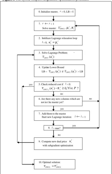
An overview of the basic steps of the hybrid simplex/subgradient optimization is given in Figure 1. The procedure iterates between column generation and Lagrange relaxation and exchanges information. We initialize the master with artificial columns and/or a feasible heuristic solution (Step 0). Next we solve the master a first time (r = 1) with the simplex method, giving v_DWCLr , the objective value of the current master at step r, and the dual prices

r t

µ on the capacity constraints and π_ir on the convexity constraints (Step 1). Next we switch to Lagrange relaxation. We set the Lagrange multipliers equal to the current dual prices and initialize l, the counter for the Lagrange steps (Step 2). We solve the Lagrange problem, resulting in the lower bound v_LRCL(u_tl) (Step 3). We update the lower bound if we improve it (Step 4). At this first step in the Lagrange iteration, we have actually solved the subproblems with the optimal simplex dual prices µ_tr. We check for each item i whether we find a strictly negative reduced cost, i.e. if ( 0) 0

, − < r i t i LRCL u

v π (Step 5). If none of the columns price out, we have found the optimal solution (Step 10). Otherwise, we add the columns with a negative reduced cost to the master. Instead of continuing with the simplex reoptimization of the master, we do some iterations of the Lagrange relaxation procedure on the original problem. We increase the counter for the Lagrange iterations (Step 7) and check if it exceeds some preset maximum value (Step 8). At each step l we compute new Lagrange multipliers (Step 9) and solve a Lagrange problem with updated dual prices (Step 3). This provides us with new columns, as the Lagrange subproblem is identical to the column generation subproblem. We check if these columns are not yet in the master (Step 6). After a fixed number of Lagrange steps (Step 8), or if no new columns are added to the master (Step 6), we return to the column generation procedure. We reoptimize the master with the simplex algorithm with all the new columns added in the previous Lagrange iterations (Step 1). This gives new simplex dual prices and we continue with solving the Lagrange relaxation using these new dual prices. The procedure stops if no column prices out at the first step of a Lagrange relaxation loop (Step 5).

The advantages of this combined procedure are:

- The Lagrange lower bound can also be used as stopping criterion for the early termination of column generation.

- Between two simplex steps, new columns are generated by Lagrange relaxation. This possibly reduces degeneracy of the master.

5.4. Calculating upper bounds

Calculating feasible upper bounds during column generation is done in two ways. In a first heuristic, we start from the optimal LP solution of the current master. We round the fractional set up variables according to some cut off point. Values below the cut off point are rounded to zero, values above to one. All the set up variables are now fixed to either one or zero. Next a network problem is solved to determine the optimal production quantities for this fixed setting of the set up variables. The total cost of this feasible production plan provides an upper bound on the optimal total cost. This heuristic is repeated for different values of cut off points. This

Figure 1. The hybrid simplex/subgradient optimization procedure

2. Initiliaze Lagrange relaxation loop l = 0, r t l t u =µ 0. Initialize master, r _{= 0, LB = 0} 1. r ←r _{+ 1} Solve master: ir r t r DWCL v ,µ ,π

3. Solve Lagrange Problem: ( )

l t LRCL u

v

4. Update Lower Bound LB = ( l) t LRCL u v if ( l) t LRCL u v > LB

5. Check reduced cost if l _{= 0:} v ,(u ) 0, i P? r i l t i LRCL −π ≥ ∀∈

6. Are there any new columns which are not in t he master yet?

7. Add them to the master

Start new Lagrange iteration: l←l _{+ 1} 8. l > max?

9. Compute new dual price utl

with subgradient optimization no no yes yes no yes 10. Optimal solution: r DWCL DWCL v v =

in the solution values when increasing the cut off point. Therefore, we cut this heuristic short when the solution starts to increase. This heuristic is done at every pricing step of the column generation iteration starting from the new primal solution given by the current master. Performing the heuristic at every pricing step of the column generation process yields better results than when we do it just once at termination. A second heuristic is based on the smoothing heuristic proposed by Trigeiro et al. (1989). We take the solutions given by the subproblems and do the smoothing subroutine.

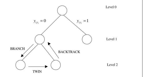
5.5. Branch-and-Price

We branch on the original set up variables yit and not directly on individual columns in the

master. By branching on the original set up variables, we actually branch on groups of columns and this normally leads to a more balanced enumeration tree (Vanderbeck 2000, Barnhart et al. 1998). The columns consisting of initial inventory only are used to maintain feasibility at each node in the branch-and-price algorithm. The branch-and-price algorithm consists of three major subroutines: branch, twin and backtrack (Figure 2). Our search strategy is depth first where branching is done on the current node. The algorithmic implementation of our formulation (20)-(25) is actually done starting from formulation (10)-(13) and the branching direction is enforced by adapting or deleting columns.

Figure 2. Building blocks of the branch-and-price algorithm

When we branch on the set up variable yit at level l in the tree, we store the following

BRANCH TWIN BACKTRACK Level 0 Level 1 Level 2 0 1 1t = i y 1 1 1t = i y

1) il refers to the item of the set up variable on which we branch at level l,

2) tl refers to the time period of the set up variable on which we branch at level l,

3) the branch direction: up (U) to one, i.e. yit = 1, or down (D) to zero, i.e. yit = 0,

4) l

i_l

F , the set of columns for item ilwhich are set to zero at level l,

5) l

i_l

C , the set of columns for item il which are modified at level l.

Let Q_i' be the set of set up schedules generated for item i so far. Further we define the available columns for item il at level l as the columns which are not set to zero at a previous

level. The set of available columns is then defined as follows:

      _∈ = − =

U

When we branch, we can fix the set up variable either to one or zero. If we branch up at level l, then we impose a set up for item il in period tl. We enforce this set up in the master

(10)-(13) by adjusting all the available columns for item il which do not have a set up in period tl.

The set of columns for item il which will be modified at this level is defined as follows:

l il C = { ∈ : =0 l l l ijt l i ss A j }

We modify these columns so that they have a set up item il in period tl:

l ljt i ss = 1 l il C j∈ ∀

Due to this extra set up, these columns obtain an extra set up cost in their objective coefficient (8) and an extra set up time in the capacity requireme nt for period tl (9):

j il c l l lj it i sc c + ← l i_l C j∈ ∀ l ljt i r l l l ljt it i st r + ← l i_l C j∈ ∀

In that way we ensure that the set up cost and set up time is properly accounted for in all the available columns according to the branching decision, even if there is no production in period tl. By adapting the columns with no set up, we avoid deleting a column at the current

step which we may have to generate again later on. In the subproblem for item il, we enforce a

set up by fixing l lt i y to one, =1 l lt i

y , but this does not necessarily imply that there must be some positive production.

If we branch down, i.e. fix a set up variable

l lt

i

y to zero, then all the available columns for item il which have a set up in period tl must be fixed at zero. The set of variables that must be

l il F = { ∈ : =1 l l l i jt l i ss A j }

This is done by imposing a simple upper bound of zero on these columns in the master: 0 ≤ j il z l il F j∈ ∀

In the subproblem, we set a high cost for that

l lt

i

y variable, so that a set up is always avoided.

Define r l DWCL

v , as the value of the master at the current level l at pricing step r. After we have

imposed the branching adjustments at level l, we solve the master, giving 0 ,l DWCL

v . If the current objective value, 0

,l DWCL

v , is larger than or equal to v_UB, our best upper bound, then we do column generation in order to see if the objective value can drop under this upper bound by generating more columns. We stop column generation at a node if no column prices out. We don’t have to investigate a node further if during column generation the lower bound on the master (35) exceeds the current upper bound v_UB. At each step of the column generation process, we also do the network and smoothing heuristic to obtain better upper bounds.

In the twin procedure at level l we have to undo the settings from the branching constraints and impose the specific adaptations for the twin for each column. There are two cases. For the twin up, we first have to undo the adaptations which we made in the branch down. We remove the simple upper bound of zero on all the columns which were adapted in the branch down at level l. These columns are in the set l

i_l F . 1 ≤ j i_l z ← _{i j} ≤0 l z l i_l F j∈ ∀

We also set the set up cost back to the original set up cost in the subproblem. After having done this, we empty the set l

i_l

F . Next we impose the specific twin up constraint, where we fix the

l lt

i

y variable to one. This is done in the same way as for the branch up.

For the twin down, we must first undo all the changes we have made in the branch up. For all the columns in which we imposed a set up for item il in period tl and hence added a set up cost

and set up time in the branch up, we must now undo this as follows:

l ljt i ss = 0 l il C j∈ ∀

This also implies that we have to subtract the set up cost again in the column cost (8) and subtract the set up time in the capacity usage (9):

j il c l l lj it i sc c − ← l i_l C j∈ ∀

l ljt i r l l l ljt it i st r − ← l il C j∈ ∀ In the subproblem, l lt i

y is no longer fixed at one, but it is binary again. The set l i_l

C is emptied. In the second step we impose the specific twin down constraint, where we fix the

l lt

i

y variable to zero. The modifications are the same as for the branch down case.

In the backtrack procedure, we must undo the adjustments that we have made in the columns at that level. There are again two cases that we have to consider. In the first case, we proceed from a twin down, so for all the columns in l

il

F a simple upper bound of zero was imposed at that level. We must undo this and set the set up cost back to the original set up cost in the subproblem. After that we empty the set l

il

F . In the second case, we proceed from a twin up, where we imposed an extra set up for all the columns in the set l

i_l

C . We undo this in the same way as in the twin down case and reset the set up variable back to binary in the subproblem. In the final step we empty the set l

i_l

C . At the end of the backtrack procedure, we go back to the previous level: l ←l−1.

6. Computational Results

We report here on the set of 540 test instances used by Trigeiro et al. (1989). All the instances have a time horizon of 20 periods and the total set consists of three subsets with 180 problems for each case of 10, 20 or 30 products. We report the averages for each class of 10, 20 and 30 products. Our algorithms were coded in Fortran using the WATCOM Fortran compiler 10.6 and linked with the LINDO library version 5.3 (Schrage 1995). The tests were done on a Pentium III 750 MHz computer under the Windows 2000 operating system. CPU times are given in seconds and the gap is calculated as the percentage difference between the best upper bound and lower bound compared to the best lower bound.

6.1. Initial Heuristics

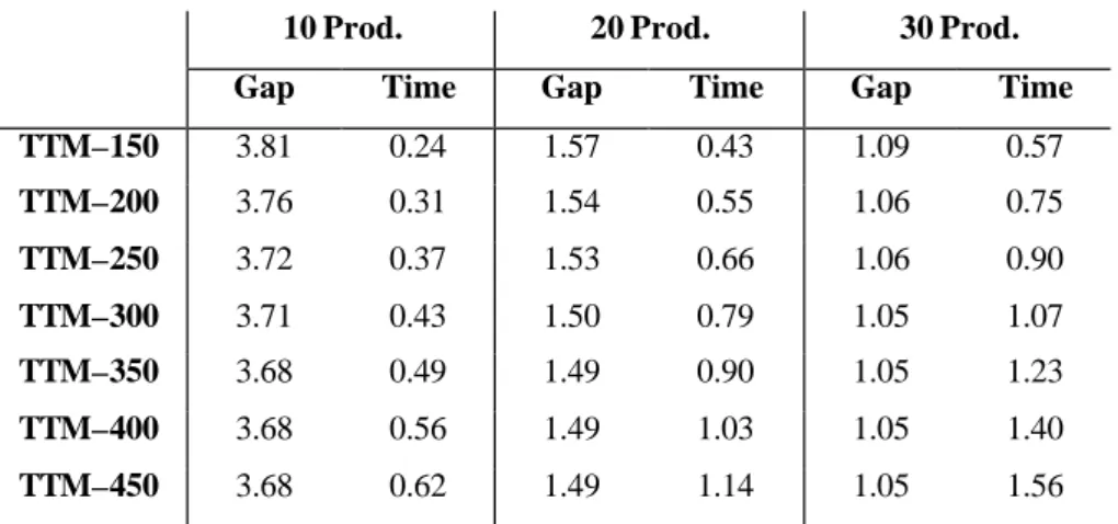
The first heuristic (TTM) is the Trigeiro et al. (1989) algorithm, using their original code. We experiment with different Lagrange iteration limits of 150, 200, 250, 300, 350, 400 and 450. In Table 1 we report on the average gap between the Lagrange lower bound and best feasible solution and the CPU time. No improvements are made after 350 iterations. For further experiments, we choose to do 300 iterations, as not much improvement is made beyond this

include this result TTM-150 in some of the next tables, so that we can see the consecutive improvements that we have made.

Table 1. Lagrange Heuristic (Trigeiro et al. 1989)

10 Prod. 20 Prod. 30 Prod.

Gap Time Gap Time Gap Time

TTM–150 3.81 0.24 1.57 0.43 1.09 0.57 TTM–200 3.76 0.31 1.54 0.55 1.06 0.75 TTM–250 3.72 0.37 1.53 0.66 1.06 0.90 TTM–300 3.71 0.43 1.50 0.79 1.05 1.07 TTM–350 3.68 0.49 1.49 0.90 1.05 1.23 TTM–400 3.68 0.56 1.49 1.03 1.05 1.40 TTM–450 3.68 0.62 1.49 1.14 1.05 1.56

Table 2 summarizes the gap and CPU time for the improvement heuristics performed after TTM. We use the network solver subroutine available in the LINDO library. The network heuristic (NH) reduces the gap further with a relatively small extra amount of CPU time. After the network heuristic, we do the lot elimination heuristic (LEH). We tested three versions. In the first version we do a full search over all the set up variables that are set at one (LEH1). In the second (LEH2) and third (LEH3) version, we do only a limited search over the first 0.3*n*m and 0.2*n*m set up variables that are at one. We always start with the items with the highest set up cost. The lot elimination heuristic reduces the gap further, but also requires a significant amount of CPU time. In the remainder of the tests, we use the second implementation (LEH2) because it gives a good trade-off between solution quality and CPU time.

Table 2. Improvement Heuristics

10 Prod. 20 Prod. 30 Prod.

Gap Time Gap Time Gap Time

TTM–150 3.81 0.24 1.57 0.43 1.09 0.57

NH 3.58 0.48 1.44 0.84 1.02 1.13

LEH1 3.27 0.59 1.34 1.24 0.94 1.98

LEH2 3.33 0.55 1.35 1.11 0.95 1.72

6.2. Solving the root node

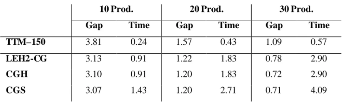
Up to now the gap is still calculated relative to the Lagrange lower bound from TTM which is equal to or lower than the optimal column generation based lower bound v_DWCL. In the next step we do the column generation at the root node to obtain this exact lower bound v_DWCL. The results are presented in Table 3. We calculate the gap for the LEH2 upper bound using the optimal lower bound obtained by column generation v_DWCL. The results are in the row LEH2-CG. The improvement from TTM-300 to LEH2 is solely due to the better upper bound. The improvement from LEH2 to LEH2-CG on the other hand is solely due to the improved lower bound. During column generation, we also perform some primal heuristics. We implement the repeated rounding heuristic (RRH) and the smoothing heuristic (SH), as discussed in Section 5. We speed up the column generation process by using the hybrid simplex/subgradient optimization procedure. Within 2 simplex iterations, we do a maximum of 25 Lagrange iterations. We report the results of the best upper bound after column generation with the hybrid method in CGH. We also report on the algorithm where we do column generation at the root node with only simplex optimization (CGS). The CGS has a substantially larger CPU time and a slightly better gap compared to CGH. With CGH, we do less pricing iterations and hence perform the heuristics (RNH and SH) fewer times. Therefore, we have less chance of finding a good upper bound. The slightly better quality of the upper bound for CGS accounts for the better gap.

Table 3. Column generation at the root node

10 Prod. 20 Prod. 30 Prod.

Gap Time Gap Time Gap Time

TTM–150 3.81 0.24 1.57 0.43 1.09 0.57

LEH2-CG 3.13 0.91 1.22 1.83 0.78 2.90

CGH 3.10 0.91 1.20 1.83 0.72 2.90

CGS 3.07 1.43 1.20 2.71 0.71 4.09

In Table 4 we compare our hybrid and regular implementation of the column generation procedure with the Eppen and Martin network reformulation (1987). In CGHLP we report the time difference between CGH and LEH2. This is actually the time to compute the exact LP lower bound with the hybrid method and do some heuristics. We compare this with the time it takes to find the LP relaxation for the variable redefinition reformulation as proposed by Eppen and Martin (EMLP), which is substantially higher. The network reformulation gives

formulation takes approximately 3, 7 and 10 times as long for the 10, 20 and 30 products. CGSLP is the time for the column generation with simplex, where we subtracted the time to calculate the LEH2 heuristic from the total time for CGS. With the hybrid optimization, it takes less than half the time to do the column generation. Further, we compare the number of columns and pricing iterations. We see that the hybrid method substantially decreases the number of pricing iterations and adds more columns.

Table 4. Hybrid versus simplex optimization and variable redefinition

10 Prod. 20 Prod. 30 Prod.

EMLP Time 1.23 5.08 12.52 CGHLP Time 0.36 0.72 1.18 CGSLP Time 0.88 1.60 2.37 CGH Cols 236.60 411.60 553.90 CGS Cols 124.40 196.20 263.30 CGH Iterations 2.31 2.32 2.24 CGS Iterations 14.24 11.47 10.38 6.3. Branch-and-Price

In our branch-and-price algorithm, we have tested 5 different branching strategies, depending on the selection of the branching variable:

B&P 1 : First fractional variable, order the items by input list,

B&P 2 : First fractional variable, order the items by decreasing set up cost, B&P 3 : Fractional variable closest to 0.5,

B&P 4 : Fractional variable closest to 0 or 1, B&P 5 : Fractional variable closest to 1.

In a heuristic implementation of the branch-and-price algorithm, we fix some of the yit

variables depending on their value in the primal solution at the end of CG at the root node. We fix all the variables below 0.05 to 0 and above 0.95 to 1. Next, we solve the smaller problem with the remaining variables optimally using the branch-and-price algorithm. We call this reduced branch-and-price (RB&P). For all the implementations reported here, we have set a limit of 2000 nodes. The summary results for the different branching strategies are given in Table 5.

Table 5. Results for the branch-and-price algorithm

10 Prod. 20 Prod. 30 Prod.

Gap Time Gap Time Gap Time

TTM–150 3.81 0.24 1.57 0.43 1.09 0.57 B&P 1 2.83 45.80 1.14 65.32 0.69 99.00 B&P 2 2.75 51.49 1.08 75.85 0.65 111.71 B&P 3 2.99 52.68 1.17 74.30 0.71 110.76 B&P 4 2.74 32.86 1.09 51.63 0.65 83.36 B&P 5 2.58 48.10 1.05 70.87 0.62 116.05 RB&P 1 2.79 20.96 1.11 26.44 0.65 31.79 RB&P 2 2.69 21.72 1.07 25.50 0.63 37.32 RB&P 3 2.84 22.46 1.10 28.72 0.64 38.11 RB&P 4 2.76 18.96 1.08 23.84 0.67 31.35 RB&P 5 2.74 24.53 1.06 27.87 0.64 35.50

On average, we obtain the smallest gaps for the fifth branching strategy, where we branch on the fractional variable closest to one. B&P4, where we branch on the variable closest to zero or one, takes on average the least CPU time, and is almost always better than B&P1, B&P2 and B&P3. The reduced branch-and-price is roughly two to three times faster compared to the optimal branch-and-price implementation. The gap can be both better or worse. RB&P2 seems to give the best gaps on average.

The data set from Trigeiro et al. that we are using here is constructed according to a full factorial experiment with 5 factors: capacity utilization (low, medium or high), number of items (10, 20 or 30), time between orders (TBO) (low, medium or high), demand variability (medium or high) and set up time (low or medium). In Table 6 we compare the effect on the gap of the different factors, as calculated with three different procedures: the TTM heuristic, with the hybrid column generation at the root node and at the end of the branch-and-price algorithm. We give separate results for the problems with 10, 20 and 30 items. In Table 7 we give the results for the CPU time.

Table 6. Gap results for the full factorial experiment

10 Prod. 20 Prod. 30 Prod.

TTM Root B&P5 TTM Root B&P5 TTM Root B&P5

Capacity Low 0.79 0.76 0.58 0.17 0.17 0.13 0.13 0.08 0.05 Usage Med. 2.23 2.01 1.48 0.65 0.62 0.49 0.29 0.29 0.24 High 8.10 6.53 5.66 3.68 2.80 2.52 2.72 1.81 1.55 TBO Low 1.91 1.59 1.51 0.94 0.67 0.64 0.75 0.42 0.39 Med. 2.54 2.28 1.77 0.99 0.89 0.76 0.62 0.50 0.43 High 6.67 5.45 4.45 2.58 2.02 1.74 1.77 1.25 1.03 Demand Med. 3.99 3.34 2.61 1.57 1.23 1.07 1.17 0.80 0.66 Var High 3.42 2.87 2.54 1.44 1.16 1.03 0.92 0.65 0.57 Set up Low 3.85 3.18 2.60 1.73 1.29 1.12 1.30 0.85 0.68 Time High 3.56 3.03 2.55 1.27 1.10 0.98 0.80 0.60 0.55 Average 3.71 3.10 2.58 1.50 1.20 1.05 1.05 0.72 0.62

Table 7. CPU times for the full factorial experiment

10 Prod. 20 Prod. 30 Prod.

TTM Root B&P5 TTM Root B&P5 TTM Root B&P5

Capacity Low 0.37 0.62 24.16 0.65 1.19 38.34 0.76 1.66 58.13 Usage Med. 0.44 0.83 44.44 0.79 1.63 73.92 1.09 2.37 118.56 High 0.49 1.29 75.70 0.92 2.68 100.35 1.36 4.68 171.46 TBO Low 0.34 0.85 36.82 0.58 1.68 46.96 0.71 2.46 83.31 Med. 0.45 0.86 50.44 0.83 1.83 77.13 1.14 2.84 118.77 High 0.51 1.04 57.04 0.94 1.98 88.53 1.37 3.41 146.08 Demand Med. 0.41 0.90 47.90 0.76 1.80 70.29 1.04 2.88 117.76 Var High 0.45 0.93 48.30 0.81 1.86 71.46 1.11 2.93 114.34 Set up Low 0.43 0.94 50.03 0.80 1.92 73.64 1.08 3.02 120.05 Time High 0.43 0.89 46.17 0.77 1.74 68.11 1.06 2.79 112.05 Average 0.43 0.91 48.10 0.79 1.83 70.87 1.07 2.90 116.05

The results here confirm the conclusions of Trigeiro et al. Demand variability and set up time have a minor effect on the gap and CPU times. The relative differences in gap between medium and high demand variability and low and high set up times seem to decrease for the solutions at the root node and at the end of the branch-and-price algorithm compared to the TTM heuristic. The capacity usage has a clear effect: if the capacity is more constrained the problems become more difficult to solve with respect to both the gap and CPU time. Problems with a higher TBO are also more difficult to solve. The effect on the gap of a low and medium TBO seems only minor, whereas the effect of a high TBO is more apparent.

In Table 8, we compare the average gap, percentage of problems that could be solved to optimality and the CPU time for the TTM heuristic and the B&P5 heuristic with 2000, 4000, 6000 and 8000 nodes. The tests reported here are performed on a 550 MHz computer. Allowing more nodes decreases the gap and increases the number of problems that could be solved to optimality, although the marginal change is decreasing. Approximately one third of the problems can be solved to optimality within 8000 nodes.

Table 8. Overview gap and percentage optimal solutions

10 Prod. 20 Prod. 30 Prod.

Gap % Opt. Time Gap % Opt. Time Gap % Opt. Time

TTM - 300 3.71 8.33 0.68 1.50 9.44 1.50 1.05 14.44 2.43

B&P 5 – 2000 2.58 23.33 86.44 1.05 29.44 141.73 0.62 32.78 231.30

B&P 5 – 4000 2.52 27.22 175.64 1.03 30.00 263.14 0.61 35.56 407.97

B&P 5 – 6000 2.48 28.89 285.83 1.02 30.00 369.20 0.60 36.11 484.81

B&P 5 – 8000 2.46 28.89 376.99 1.02 30.56 507.48 0.60 36.11 599.52

6.4. Comparison with other approaches

Other approaches have been proposed in the literature to solve the CLST. Belvaux and Wolsey (2000) describe a branch-and-cut algorithm that is specifically developed to solve lot sizing problems. They report on six instances taken from a test set used by Trigeiro et al. (1989). Belvaux and Wolsey used unit variable production times vt_it = 1 for all their data sets, whereas for one of them, specifically G30, the original data set has fractional variable production times. In Table 9 we report the results for the test problems. G30b refers to the G30 data set with unit variable production times. Belvaux and Wolsey use a 200MHz computer under Windows NT and set a time limit of 900 seconds. We have a limit of 2000 nodes. Altough we cannot make any robust conclusion based on such a limited comparison, the branch-and-cut system seems to perform better on the smaller problems and our algorithm seems to perform slightly better on the larger problems. For the smaller problems their branch-and-cut algorithm gives a better lower bound at the root node, whereas for the larger problems both procedure yield the same lower bound. The results indicate that these CLST problems are indeed hard to solve.

Table 9. Comparison branch-and-cut and branch-and-price

Branch-and-Cut Belvaux and Wolsey (2000)

Branch-and-Price (B&P5)

LP IP Time Gap LP IP Time Gap

Tr6-15 (G30) - - - - 37,103.1 37,809 33.3 1.90 Tr6-15(G30b) 37,213.3 37,721(1) 38.4 1.09 37,201.2 38,162 29.0 2.51 Tr6-30 (G62) 60,979.4 61,806 900 1.36 60,946.2 62,644 359 2.79 Tr12-15 (G53) 73,858.2 74,799 900 1.27 73,847.9 75,035 66 1.61 Tr12-30 (G69) 130,177 132,650 900 1.90 130,177.2 131,234 215 0.81 Tr24-15 (G57) 136,366 136,872 900 0.37 136,365.7 136,860 44 0.36 Tr24-30 (G72) 287,753 288,424 900 0.23 287,753.4 288,383 306 0.22

The network formulation (Eppen and Martin 1987) was solved with the MIP solver of LINDO. For 10 and 20 products, we set a pivot limit of ten million, for the 30 products we set a pivot limit of 5 million. From Table 10 we observe that the algorithm is slower and does not give the same good quality solutions as our procedure.

Table 10. Variable redefinition results

10 Prod. 20 Prod. 30 Prod.

Gap Time Gap Time Gap Time

TTM–150 3.81 0.24 1.57 0.43 1.09 0.57

EMIP 4.49 2,949 2.94 6,077 2.35 4,904

Gapolakrishnan et al. (2001) develop a customized tabu search algorithm for the CLST. They test their procedure on the data set from Trigeiro et al. with the 540 problem instances and report an average gap of 4.01% and an average CPU time of 97 seconds on a Pentium, 550 MHz processor. With our algorithm, we obtain an average gap of 1.67% and an average CPU time of 1.9 seconds at the root node (CGH). For our branch-and-price implementation (B&P5), we have an average gap of 1.42% and average time of 79 seconds. Our algorithm is clearly superior to the tabu search.

6.5. Some more results

We have also tested our procedure on other data sets from Trigeiro et al. (1989). These are 70 instances from the F-set and 71 from the G-set. All the instances in the F set are 6 products and 15 period problems. The G-set consists of 46 instances with 6 products and 15 periods and 5 instances for each of the cases with 12 products and 15 periods, 24 products and 15 periods, 6 products and 30 periods, 12 products and 30 periods and 24 products and 30 periods. In Table 11, we give the gap and time for the initial heuristic, which includes TTM, NH and LEH2, for the column generation at the root node and for the branch-and-price algorithm using B&P5 with a 2000 node limit. We compare this to the Eppen and Martin formulation solved by LINDO with a maximum of 5 million pivots. Our branch-and-price algorithm performs better than the network reformulation.