Automatic SIMD vectorization for Haskell

Kent Academic Repository

Full text document (pdf)

Copyright & reuse

Content in the Kent Academic Repository is made available for research purposes. Unless otherwise stated all

content is protected by copyright and in the absence of an open licence (eg Creative Commons), permissions

for further reuse of content should be sought from the publisher, author or other copyright holder.

Versions of research

The version in the Kent Academic Repository may differ from the final published version.

Users are advised to check

http://kar.kent.ac.uk

for the status of the paper.

Users should always cite the

published version of record.

Enquiries

For any further enquiries regarding the licence status of this document, please contact:

[email protected]

If you believe this document infringes copyright then please contact the KAR admin team with the take-down

information provided at

http://kar.kent.ac.uk/contact.html

Citation for published version

Petersen, Leaf and Orchard, Dominic A. and Glew, Neal (2013) Automatic SIMD vectorization

for Haskell. In: ACM SIGPLAN International Conference on Functional Programming, 25

- 27 Sep 2013, Boston, MA, USA.

DOI

https://doi.org/10.1145/2500365.2500605

Link to record in KAR

http://kar.kent.ac.uk/57494/

Document Version

Automatic SIMD Vectorization for Haskell

Leaf Petersen

Dominic Orchard

Neal Glew

Abstract

Expressing algorithms using immutable arrays greatly simplifies the challenges of automatic SIMD vectorization, since several im-portant classes of dependency violations cannot occur. The Haskell programming language provides libraries for programming with immutable arrays, and compiler support for optimizing them to eliminate the overhead of intermediate temporary arrays. We de-scribe an implementation of automatic SIMD vectorization in a Haskell compiler which gives substantial vector speedups for a range of programs written in a natural programming style. We com-pare performance with that of programs compiled by the Glasgow Haskell Compiler.

Categories and Subject Descriptors D.3.4 [Programming Lan-guages]: Processors—Compilers; D.3.4 [Programming Languages]: Processors—Optimization; D.1.1 [Programming Techniques]: Ap-plicative (Functional) Programming

Keywords Vectorization, SIMD, Compiler Optimization, Haskell, Functional Languages

1.

Introduction

In the past decade, power has increasingly been recognized as the key limiting resource in micro-processors, in part due to the limited battery on mobile devices, but more fundamentally due to the non-linear scaling of power usage with frequency. This has forced micro-processor designs to explore (or re-explore) different avenues at both the micro-architectural and the architectural levels. One successful architectural trend has been the increasing emphasis on data parallelism in the form of single-instruction multiple-data (SIMD) instruction sets.

The key idea of data parallelism is that significant portions of many sequential computations consist of uniform (or almost uni-form) operations over large collections of data. SIMD instruction sets exploit this at the machine instruction level by providing data paths for and operations on fixed-width vectors of data. Program-mers (or preferably compilers) are then responsible for finding data parallel computations and expressing them in terms of fixed-width vectors. In the context of languages with loops (or compiled to loops), this corresponds to choosing loops for which multiple it-erations can be computed simultaneously.

Permission to make digital or hard copies of all or part of this work for personal or classroom use is granted without fee provided that copies are not made or distributed for profit or commercial advantage and that copies bear this notice and the full citation on the first page. Copyrights for components of this work owned by others than the author(s) must be honored. Abstracting with credit is permitted. To copy otherwise, or republish, to post on servers or to redistribute to lists, requires prior specific permission and/or a fee. Request permissions from [email protected].

ICFP’13_{, September 25–27, 2013, Boston, USA.}

Copyright is held by the owner/author(s). Publication rights licensed to ACM. ACM 978-1-4503-2326-0/13/09. . . $15.00.

http://dx.doi.org/10.1145/2500365.2500605

The task of automatically finding SIMD vectorizable code in the context of a compiler has been the subject of extensive study over the course of decades. For common imperative programming languages, such as C and Fortran, in which programs are structured as loops over mutable arrays of data, the task of rewriting loops in SIMD vector form is straightforward. However, the task of discov-ering which loops permit a valid rewriting (via dependency analy-sis) is in general undecidable, and has been the subject of extensive research (see e.g. [13] and overview in [15]). Even quite sophisti-cated compilers are often forced to rely on programmer annotations toassertthat a given loop is a valid target of SIMD vectorization (for example, theINDEPENDENTkeyword in HPF [7]).

A great deal of the difficulty in finding vectorizable loops sim-ply goes away in the context of a functional language. In functional languages, the absence of mutation eliminates large classes of the more difficult kinds of dependence violations that block vectoriza-tion in compilers for imperative languages. In this sense, SIMD vectorization would seem to be quite low-hanging fruit for func-tional language compiler writers. In this paper, we describe the implementation of an automatic SIMD vectorization optimization pass in the Intel Labs Haskell Research Compiler (HRC). We argue that in a functional language context, this optimization is straight-forward to implement and gives excellent results.

HRC was originally developed to compile programs written in an experimental strict functional language, and the vectorization optimization that we present here was developed in that context. However, the main bulk of our compiler infrastructure was de-signed to be fairly language agnostic, and we have more recently used it to build an experimental Haskell compiler using the Glas-gow Haskell Compiler (GHC) as a front end. While Haskell is quite a complex language on the surface, the GHC front end reduces it to a relatively simple intermediate representation based on System F, which is fairly straightforward to compile using HRC. By inter-cepting the GHC intermediate representation (IR) after the main high-level optimization passes have run, we gain the benefit of the substantial and sophisticated optimization infrastructure built up in GHC, and in particular we benefit from its ability to optimize away temporary intermediate arrays.

We make the following three contributions:

• We design a core language with arrays and SIMD vector

prim-itives (Section 3).

• We present a detailed compositional vectorization process over

this language (Section 4).

• We evaluate our performance compared to GHC with the native

and LLVM backends, showing significant scalar speedups over GHC and additional vector speedups of up to6.5×over our own scalar compiler, on a selection of array processing bench-marks (Section 5).

We begin with a brief overview of HRC and its relationship to GHC.

2.

Intel Labs Haskell Research Compiler

HRC provides an optimization platform aimed at producing high-performance executables from functional-style code. The core in-termediate language of the compiler is a static single-assignment style, control-flow graph based intermediate representation (IR). It is strict and has explicit thunks to represent laziness. While the intermediate representation is largely language agnostic, it is not paradigm agnostic. The core technologies of the compiler are designed specifically around compiling functional-language pro-grams. Most importantly for the purposes of this paper, the com-piler relies on maintaining a distinction between mutable and im-mutable data, and focuses almost all of its optimization effort on the latter. The compiler is structured as a whole-program compiler— however, none of the optimizations in the compiler rely on this property in any essential way. In addition to the usual inlining-style optimizations, contification [5] is performed to turn many uses of (mutual) recursion into loops. This optimization is crucial for our purposes since we structure our SIMD-vectorization optimization as an optimization on loops. Many standard compiler optimizations have been implemented in the compiler, including loop-invariant code motion and a very general simplifier in the style of Appel and Jim [2]. The compiler also implements a number of inter-procedural representation optimizations using a field-sensitive flow analysis [11].

The compiler generates output in a modified extension of the C language calledPillar[1]. Among other things, the Pillar lan-guage supports tail calls and second-class continuations. Most im-portantly, it also provides the necessary mechanisms to allow for accurate garbage collection of managed memory. While an early version of Pillar was implemented as a modification of a C com-piler, Pillar is currently implemented as a source to source transla-tion targeting standard C, which is then compiled using either the Intel C Compiler or GCC. Our garbage collector and a small run-time are linked in to produce the final executable.

2.1 Haskell and GHC

The Haskell language and the GHC extensions to it provide a large base of useful high-level libraries written in a very powerful pro-gramming language. These libraries are often written using a high-level functional-language style of programming, relying on excel-lent compiler technology to achieve good performance. While we wished to compile Haskell programs and take advantage of the many libraries, we had no interest in attempting the monumental task of duplicating all of the high-level compiler technology imple-mented in GHC. The approach we took therefore was to essentially use GHC as a Haskell frontend, thereby taking advantage of the existing type-checker and high-level optimizer.

GHC provides some support for writing its main System-F-style internal representation (called Core) out to files. While this code is not entirely maintained, we were able to easily modify it to support all the current Core features we require. We use this facility to build a Haskell compiler pipeline by first running GHC to perform type checking, desugaring, and all of its Core-level optimizations, and then writing out the Core IR immediately before it would otherwise be translated to the next-lower representation. HRC then reads in the serialized Core, and after several initial transformations and optimizations (including making thunks explicit), performs a closure-conversion pass and transforms it down to our main CFG based intermediate representation for subsequent optimization.

2.2 GHC Modifications

Using this approach, we are able to provide a fairly close to func-tionally complete implementation of the Haskell language as im-plemented by GHC. However, some of the choices of primitives used in GHC do not match up well with the needs of HRC, and so

some modification of GHC itself was required. A notable example of this for the purposes of this paper is the treatment of arrays in the Data.Vector libraries.

The GHC libraries Data.Vector and REPA [6] provide clean high-level interfaces for generating immutable arrays. Program-mers can use typical functional-language operations like maps, folds, and zips to compute arrays from other arrays. These oper-ations are naturally data parallel and amenable to SIMD vector-ization by HRC. For example, consider a map operation over an immutable array represented with the Data.Vector library. Such ar-rays are represented internally to the libraries using streams, and so map first turns the source array into a stream, applies the map operation to the stream, and then unstreams that back into the final array. Unstreaming is implemented by running a monadic compu-tation that first creates a mutable array of the appropriate size, then initializes the elements of the array using array update, and finally does an unsafe freeze of the mutable array to an immutable array type [8]. GHC has optimizations which usually eliminate all of the intermediate streaming, mapping, and unstreaming operations. The result of this optimization is a piece of code that sequences the array creation, the calling of a tail-recursive function that initial-izes the array elements, and the unsafe freeze. After translation into our internal representation, HRC can then contify the tail-recursive function into a loop, resulting in a natural piece of code that can be effectively optimized using standard loop-based optimizations adapted to leverage the benefits of immutability.

Unfortunately, observe that as described in the previous para-graph we do not actually get the benefits of immutability with an unmodified GHC. Instead, we end up with code that creates a mutable array and then initializes it with general array update operations—a style of code that we argue is drastically harder to optimize well in general, and to perform SIMD vectorization on in particular. As we discuss in Section 4.7, immutable arrays make determining when a loop can be SIMD vectorized much easier. For our purposes then, what we would like GHC to generate instead of the code described above is code that creates a new uninitialized immutable array and then usesinitializing writesto initialize the array. The two invariants of initializing writes are that reading an array element must always follow the initializing write of that ele-ment, and that any element can only be initialized once. This style of write preserves the benefits of immutability from the compiler standpoint, since any initializing write to an element is the unique definition of that element. Initializing writes are key to representing the initialization of an immutable array using the usual loop code, while preserving the ability to leverage immutability.

In order to get immutable code written in this style from GHC and the libraries discussed above, we modified GHC with new primitive immutable array types1and primitive operations on them. The additional operations include creation of a new uninitialized array, initializing writes, and a subscript operation. We also mod-ified the Data.Vector library and a small part of the REPA library to use these immutable arrays instead of mutable arrays and unsafe freeze (of course, as with the standard GHC primitives, correctness requires that the library writer use the primitives correctly). With these modifications, the code produced by GHC is suitable for op-timization by HRC, including in many cases SIMD vectorization.

2.3 Vectorization in HRC

SIMD vectorization in HRC targets loops for which the compiler can show that executing several iterations in parallel is seman-tics preserving, rewriting them to use SIMD vector instructions. Usually these loops serve to initialize immutable arrays, or to

per-1_{GHC does already have some such types—however, we added new ones}

Register kind k ::= s|v Variables xk_{, y}k_{, z}k_{, . . .} Constants c ::= −231 , . . . ,(231 −1) Operations op ::= +,−,∗, /, . . . Instruction I ::= zs_=c | zv_=hxs 0, . . . , xs7i | zs_=xv_!i | zs_=op(xs 0, . . . , xsn) | zv_=hopi(xv 0, . . . , xvn) | zs₌ new[xs_] | zs_=xs_[ys_] | zv_=xs_[hyv_i] | zv_=hxv_i[ys_] | zv_=hxv_i[hyv_i] | xs_[ys_]←zs | xs_[hyv_i]←zv | hxv_i[ys_]←zv | hxv_i[hyv_i]←zv Comparisons cmp ::= xs _{< y}s_|xs _{≤ y}s_|xs _{= y}s Labels L ::= L0,L1, . . . Transfers t ::= gotoL(xk 0, . . . , xkn) | if(cmp)gotoL0(xk0, . . . , xkn) else gotoL1(y0k, . . . , ykm) | halt Blocks B ::= L(xk 0, . . . , xkn): I0 . . . Im t

Control Flow Graph ::= EntryLin{B0, . . . , Bn} Figure 1. Syntax

form reductions over immutable arrays. The compiler generates the SIMD loops and all of the related control logic simply as code in our intermediate language. Rather than requiring the compiler to generate only the SIMD instructions provided by the target ma-chine, we provide a more uniform SIMD instruction set that may be a superset of the machine-supported instructions. Our small run-time provides a library of impedance-matching macros that imple-ments the uniform SIMD instructions in terms of SIMD intrisics understood by the underlying C compiler. The C compiler is then responsible for low-level optimizations including register alloca-tion and instrucalloca-tion selecalloca-tion.

In the next section we define a vector core language with which to discuss the vectorization process. This core language is clean, uniform, and is almost exactly faithful to (a small subset of) our actual intermediate representation.

3.

Vector Core language

We define here a small core language in which to present the vec-torization optimization. We restrict ourselves to an intra-procedural fragment only, since for our purposes here we are not interested in inter-procedural control flow. Programs in the language are given as control-flow graphs written in a variant of static single-assignment (SSA) form. To keep things concrete, our language is based on a 32-bit machine with vector registers that are 256-32-bits wide; handling other register and vector widths is a straightforward extension.

3.1 Objects

The primitive objects of the vector core language consist of heap objects and register values. Heap objects are variable-length

im-mutable arrays subscripted by 32-bit integers. The elements con-tained in the fields of heap objects are constrained to be 32-bit reg-ister values. Regreg-ister values are small values that may be bound to variables and are implicitly represented at the machine level via registers or spill slots. The register values consist of 32-bit integers, 32-bit pointers to heap values, and 256-bit SIMD vectors each con-sisting of eight 32-bit register values. Adding additional primitive register values such as floating-pointer numbers, booleans, etc. is straightforward and adds nothing essential to the presentation.

3.2 Variables

Variables are divided into two classes according to size: scalar variablesxs_{that may only be bound to 32-bit register values and}

vector variablesxv_{that may only be bound to 256-bit vector values.}

In practice of course, a real intermediate language will also have additional variable sizes: 64-bit variables for doubles and 64-bit integers, and a range of vector widths possibly including 128- and 512-bit vectors. Note that the variablesxs_andxv_{are considered}

to be distinct variables. Informally, we will sometimes usexv _to

denote the variable containing a vectorized version of an original program variablexs_{—however, this is intended to be suggestive}

only and has no semantic significance.

3.3 Instructions

The instructions of the vector language serve to introduce and oper-ate on the primitive objects of the language. Most of the instructions bind a new variable of the appropriate register kind, with the excep-tion of the array-initializaexcep-tion instrucexcep-tions which write values into uninitialized array elements. The move instructionzs _{= c}

binds a variable to the 32-bit integer constantc. The vector introduction instructionzv_=hxs

0, . . . , xs7ibinds the vector variablezvto a

vec-tor composed of the contents of the eight listed 32-bit variables. We use the derived syntaxzv _=hcs

0, . . . , cs7ito introduce a vector of

constants—this may be derived in the obvious way by first binding each of the constants to a fresh 32-bit variable. A component of a vector may be selected out using the select instructionzs _=xv_!i,

which bindszs_{to theith component of the vector inx}v_(wherei

must be in the range0. . .7). The instructionzs ₌

op(xs

0, . . . , xsn)corresponds to a family

of instructions operating on primitive 32-bit integers, indexed by the operationop(e.g. addition, subtraction, negation etc.). Primitive operations must be fully saturated—that is, the number of operands provided must equal the arity of the given operation. We lift the primitive operations on integers to pointwise primitive operations

on vectors with thezv _{= h}

opi(xv

0, . . . , xvn) instruction, which

appliesoppointwise across the vectors. That is, semanticallyzv₌

hopi(xv

0, . . . , xvn)behaves identically to a sequence of instructions

performing the scalar version ofopto each of the corresponding elements of the argument vectors, and then packaging up the result as the final result vector.

Array objects in the vector language are immutable sequences of 32-bit data allocated in the heap. New uninitialized array objects are allocated via thezs ₌

new[xs_{]instruction which allocates a}

new array of lengthxs_(wherexs_{must contain a 32-bit integer) and}

bindszs_{to a pointer to the array. The initial contents of the array}

are undefined, and every element must be initialized before being read. It is an unchecked invariant of the language that every element of the array is initialized before it is read, and that every element of the array is initialized at most once. It is in this sense that the arrays are immutable—the write operation on arrays serves only as an initializing write but does not provide for mutation. Ordinary scalar element initialization is performed via the xs_[ys_{] ← z}s

operation which initializes the element of arrayxs

at offsetys

to

zs

instruction, which reads a single element from the arrayxs_{at offset}

ys_{and bindsz}s_{to it.}

In order to support SIMD vectorization, the vector language also provides a general set of vector subscript and initialization operations permitting vectors of elements to be read from and written to arrays (or vectors of arrays) in a single instruction. The set of instructions we provide are more general than what is supported by most existing machine architectures. This is done intentionally since it is often beneficial to vectorize a loop even if some instructions must be emulated via translation to scalar operations. Moreover, we believe it is useful to present the language in its most general form—it is always possible to restrict the set of generated instructions as desired. We defer discussion of the situations in which these various styles of loads and stores arise to subsequent sections on the actual vectorization operation.

The simplest vector array loads and stores are the operations that read multiple elements directly from a single array into a vector variable, or initialize multiple elements of a single array with elements contained in a vector variable. The instructionzv₌

xs_[hyv_{i]takes a single arrayx}s_{and a vector of offsetsy}v_{and binds}

zv_{to a vector containing the elements ofx}s_{from the given offsets.}

That is, semantically we may treat the instructionzv_=xs_[hyv_i]as

equivalent to the following list of instructions:

ys 0 =yv!0 zs 0 =xs[ys0] . . . ys 7 =yv!7 zs 7 =xs[ys7] zv _=hzs 0, . . . , z7si

This instruction is commonly known as a “gather” instruction. The initializing storexs_[hyv_i]←zv_{, commonly known as the “scatter”}

instruction, writes the elements of the vectorzv_{to the fields ofx}s

at offsets given by the vectoryv_.

There are several interesting special cases of scatters and gathers that are worth further discussion. A common idiom that arises in SIMD vectorization consists of array loads and stores such that the index vector is constructed by adding multiples of a constant stride to a scalar index. We choose to introduce this idiom as derived syntax as follows, whereiis a constant valued stride:

zv_=xs_[hys_:ii] def =zv_=xs_[hyv_i] xs_[hys_:ii]←zvdef =xs_[hyv_i]←zv where    yv l =hys, . . . , ysi yv b =h0, . . . ,7∗ii yv_=h+i(yv l, ybv)

Note that the stride multiplications (e.g.7∗i) are meta-level oper-ations. We also provide derived syntax for the further special case in which the stride is known to be one:

zv_=xs_[hys_:i] def

= zv_=xs_[hys_:1i]

xs_[hys_:i]←zvdef

= xs_[hys_:1i]←zv

For the purposes of simplicity of the vector language, we have left these as derived forms. However, it is worth noting that many archi-tectures provide support for these idioms directly (and in fact may provide supportonlyfor these idioms) and hence from a pragmatic standpoint it can be important to provide primitive support for these addressing modes.

A second mode of addressing for array loads and stores covers the case where a vector of arrays is indexed pointwise by a single fixed scalar offset. Thezv_=hxv_i[ys_{]instruction produces a vector}

zv

such that theith element ofzv

is produced by indexing theith array from the vector of arraysxv

, using offsetys

. Similarly, the

hxv_i[ys_]←zv_{instruction sets the element of theith array in the}

vectorxv_{at offsety}s_{to the value in theith position ofz}v_.

The final mode of addressing for array loads and stores covers the case in which a vector of arrays is indexed pointwise using a vector of offsets. Thezv _{= hx}v_i[hyv_{i]instruction produces a}

vectorzv _{such that theith element is produced by indexing the}

ith array from the vector of arraysxv_{using theith offset from the}

vector of offsetsyv_{. Similarly, thehx}v_i[hyv_{i] ← z}v _instruction

sets the element of theith array in the vectorxv_{at the offset given}

by theith element of the vector of offsetsyv_{to the value in theith}

position ofzv

.

3.4 Basic Blocks

Instructions are grouped into basic blocks consisting of a labeled entry, a sequence of instructions, and a transfer which terminates the block and either transfers control to another block or terminates the program. We assume an infinite supply of distinct program labels ranged over by metavariableLused to label basic blocks that we distinguish by numbering distinct labels with distinct integers (asL0,L1, etc.).

Basic block headers consist of the label of the block and a list of entry variables which are defined on entry to the block. The entry variables are given their defining values by the transfer which transfers control to the block. Block entry variables may have scalar or vector kind.

Transfers terminate basic blocks, and serve to transfer control within a program. ThegotoL(xk

0, . . . , xkn)transfer shifts control

to the block labeled with L. Well-formed programs must have

matching arities on transfers and the block headers which they target, that is, the block labeled withLmust have entry variables

zk

0, . . . , zkn. The transfer of control effected bygotoL(xk0, . . . , xkn)

also defines the entry variables zk

0, . . . , znk to be the values of

xk

0, . . . , xkn.

The conditional control transfer

if(cmp)gotoL0(xk0, . . . , x

k

n)else gotoL1(y0k, . . . , y

k m)

behaves asgotoL0(xk0, . . . , xkn)if the comparison holds, and as gotoL1(y0k, . . . , ymk)if the comparison does not hold. Note that

the targets of the two different arms of the conditional are not required to be distinct.

Thehalttransfer terminates the program. We do not consider inter-procedural control-flow in this core language since it is not relevant to the vectorization optimization—however it is straight-forward to add additional transfers to account for this if desired.

3.5 Programs

Programs in the core language consist of a single control flow graph. A control flow graph consists of a designated entry label L and set of associated basic blocks, each with a distinct label, one of which (the entry block) is labeled with the entry labelL. The entry block must expect no entry variables. Program execution proceeds by starting at the designated entry block and executing block instructions and transfers until ahaltinstruction is reached (if ever). Well-formed programs must not contain transfers whose target label is not in the control-flow graph, and every block in the control-flow graph must be labeled with a distinct label. As usual with static single-assignment form, variables may only be defined once, must be defined before their first use, and have scope given by the dominator tree of the control-flow graph rooted at the entry label. The style of static single-assignment form used in this core language is similar to that used in compilers such as the MLton compiler [16].

4.

Vectorization

The SIMD-vectorization optimization attempts to rewrite a loop to a new loop that executes multiple iterations of the original loop on each iteration using SIMD instructions and registers. While the core idea is quite simple, there are a number of issues that must be addressed in order to preserve the semantics of the original program. In the first part of this section we introduce the key issues using a series of examples. Before doing so, we first review some preliminary concepts.

4.1 Loops

We have informally described our vectorization efforts as focusing on loops. Loops tend to account for a high proportion of executed instructions in programs, and as such are natural targets for intro-ducing SIMD-vector code. We define loops using the standard no-tion of a natural loop, merging loops with shared headers in the usual way to ensure that the nesting structure of loops form a tree. We do not assume a reducible control-flow graph (since in general the translation of mutually-recursive functions into loops may in-troduce irreducible control flow). We focus our vectorization efforts more specifically on the innermost loops that make up the leaves of the loop forest of the control-flow graph. For simplicity, we only target bottom-test loops. A separate optimization pass inverts top-test loops to form bottom-top-test loops, both to enable vectorization and loop-invariant code motion.

4.2 Induction variables

Our notion of induction variable is standard, but we review it in some detail here since induction variables play a critical role in our algorithm. We define thebaseinduction variables of a loop to be the entry variables of the entry block of the loop such that the definition of that variable provided on the loop back edge is produced by adding a constant to the variable itself, and where the initial value passed into the loop is a compile-time constant. The stepof a base induction variable is the constant added each time around the loop. The full set of induction variables is the least set of variables satisfying:

•A base induction variable is an induction variable.

•A variable defined byxs= +(ys, zs), whereysis an induction

variable andzs

is a constant (defined byzs_=c

), is an induction variable.

•A variable defined byxs=∗(ys, zs), whereysis an induction

variable andzs_{is a constant, is an induction variable.}

Our implementation also deals with the symmetric versions of the last two cases, and also considers operations such as subtraction and negation. Arbitrary initial values can be allowed for base in-duction variables and loop invariants can be allowed in place of constants at the cost of some additional complexity as discussed below, but we do not currently support this.

Induction variables can be characterized as affine functions of the iteration count of the loop. The characteristic function for an induction variableis

is an equation of the formis_=p∗#+d

where

pis a constant (the step of the induction variable), anddis also a constant (the initial value of the induction variable). The symbol# stands for the iteration number: the value of the induction variable

is_{for iterationjcan be computed directly from its characteristic}

function simply by replacing#withj.

The characteristic function for an induction variable is derived as follows:

•The characteristic function of a base induction variable isp∗

# +dwherepis the step of the base induction variable as defined above, anddis the constant initial value of the induction variable.

• The characteristic function of an induction variable defined by

xs_{= +(y}s_{, z}s_{)isp∗# +d+cwherez}s_{is a constant (defined}

byzs_{=c), andp∗# +dis the characteristic function ofy}s_. • The characteristic function of an induction variable defined by

xs_=∗(ys_{, z}s_{)isc∗p∗#+c∗dwherez}s_{is a constant (defined}

byzs_{=c), andp∗# +dis the characteristic function ofy}s_.

A subtle but important point is that in these computations the com-piler must ensure that the overflow semantics of the underlying meric type are respected to avoid introducing or eliminating nu-meric overflow. It is possible to extend the definition of charac-teristic functions to allow loop invariants to take the place of the constants in the above definition at the expense of representing the characteristic function symbolically, thereby somewhat complicat-ing code generation and overflow avoidance as discussed below.

4.3 Vectorization by example

Consider the following simple program which computes the point-wise sum of two arraysbs

andcs , each of lengthls . L0(): as₌ new[ls_] is 0= 0 goto L1(is 0) L1(is_): xs_=bs_[is_] ys_=cs_[is_] zs_{= +(x}s_{, y}s₎ as_[is_]←zs is 1= +(is,1) if(is 1 < ls)goto L 1 (is 1)

else goto Lexit(is

1)

(1)

Ignoring the crucial issue of whether or not it is in factvalid to vectorize this loop, there are a number of issues that need to be addressed in order to produce a vector version of this program.

4.3.1 The vector loop

The core of the vectorization optimization is to produce an inner loop, each iteration of which executes multiple iterations of the original loop. For Example 1, this corresponds to generating code to vector-load eight elements of the arraysbandcat appropriate offsets, perform a pointwise vector addition of the loaded elements, and to perform a vector write of the eight result elements into the new arraya. The comparison which controls the exit test at the bottom of the loop must also be adjusted appropriately to account for the fact that multiple iterations are being performed. Finally, on the exit edge of the loop, the use of the last value of the induction variableis

1must also be accounted for.

To motivate the general treatment of the vectorization optimiza-tion, we first consider the individual instructions of Example 1, be-ginning with the load instructionxs _{= b}s_[is_{]. Executing this}

in-struction during iterationjof the loop loads a single element from the arraybs

at an offset given by the value ofis

. In the vector loop, we wish to perform iterationsj, j + 1, . . . , j+ 7 simulta-neously. The vector version of this instruction then must load eight elements frombs _{at offsets given by the values ofi}s _{at iteration}

j, j+ 1, . . . , j+ 7. A natural first attempt at vectorization might be to simply assume that vector versions of all variables are available, and to then generate the corresponding vector instruction using the vector variables. In this case, if we assume the existence of vari-ablesbv _{and i}v _{containing the values ofb}s _andis _{for iterations}

j, . . . , j+ 7then the vector instructionxv _=hbv_i[hiv_{i]puts into}

xv_{the appropriate values ofx}s_{for iterationsj, . . . , j+ 7.}

While this approach is correct (and in the most general case is sometimes necessary) a key insight in SIMD vectorization is that it is often possible to do much better by using knowledge of loop invariants and induction variables. In this case, the variablebs _is

loop invariant, and consequentlybv _{will consist simply of eight}

copies of the same value. Semantically then, we can replace our use of the general vector load instruction with the simpler gather

instructionxv _{= b}s_[hiv_{i], which does not require us to produce}

the vector version ofbs_{and which may also have a more efficient}

implementation. More importantly, the variableis _{here is a base}

induction variable with step1. It is consequently possible to predict the value ofis_{at each of the next eight iterations: that is, the value}

ofiv_{will always behi}s_{, i}s_{+1, . . . , i}s_{+7i. The vector load can then}

be seen to be a load of eight contiguous elements frombs_{, for which}

we have provided the derived instructionxv _{= b}s_[his_{:i], which}

performs a contiguous load of eight elements, as desired. Since this form of load is generally well supported in vector hardware, generating this specialized form in preference to the general form is highly desirable.

The second load instruction can then be vectorized in an exactly analogous fashion, resulting in two vector variablesxv_andyv_{. The}

addition instructionzs _{= +(x}s_{, y}s_{)can then be computed using}

vector addition on the vector variables, aszv _=h+i(xv_{, y}v_{). To}

produce a vector version of the instruction as_[is_{] ← z}s _which

writes the computed value to the new array we follow a similar argument to that above for the loads to produce theas_[his_:i]←zv

instruction which performs a contiguous write of the values inzv

into the arrayas_{starting at offseti}s_.

The last instruction of the loop,is

1 = +(is,1), is the induction

variable computation, and as such requires special treatment. The result of this instruction is used for three purposes: in the computa-tion of the test to decide whether to proceed with another iteracomputa-tion, to provide a new value for the induction variable in the next itera-tion, and to provide the value passed out on the exit edge.

For the latter two uses, the required value is easy to see. Each iteration of the vector loop corresponds to eight iterations of the scalar loop, and we require on entry to the loop that the induction variableis _{contain the value appropriate for the first of the eight}

iterations. Given the value ofis_{for iterationjthen, the back edge}

of the loop requires the value ofis

1for iterationj+ 7, which is one

plus the value ofis_{on iterationj+ 7. Similarly, the exit edge of the}

loop requires the value ofis

1at iterationj+7. Since the computation

of the value ofis_{for each iteration depends on the value of itself}

in the previous iteration, we might imagine ourselves to be stuck. However, the nature of induction variables as affine transformations means that we can compute the value ofis

1at iterationj+7directly:

each iteration adds1to the original value, hence the value ofis_at

iterationj+ 7is given byis_{+ 7, and the value ofi}s

1at iteration

j+ 7isis_{+ 7 + 1. Hence we can compute the appropriate value}

ofis

1for both the back and the exit edge asis+ 8.

The remaining use of the induction variableis

1is to compute the

loop exit test. The key insight is that it is no longer sufficient to check that there is at least one iteration remaining: in order to exe-cute the vector loop again, we must have at least eight remaining erations. Upon completion of a vector iteration computing scalar it-erationsj, . . . , j+7, the question that must be answered is whether the scalar loop would always execute iterationsj+ 8, . . . , j+ 15. Because of the monotonic nature of the induction variable compu-tation this in turn can be reduced to the question of whether or not the value ofis

1at iterationj+ 14is less thanls. Sinceis1is an

in-duction variable which is incremented by1on each iteration, this corresponds to changing the exit test to ask whetheris_{+ 15 < l}s_. 4.3.2 Entry and exit code

Using the ideas from previous section, it is straightforward to write a vector version of the core loop. In addition to the issues touched on above, vectorizing this example also requires accounting for the possibility that there may be insufficient iterations to allow use of the vector loop, and also for the possibility that there may be extra iterations left over if the exit test succeeds with fewer than eight but more than zero iterations left. To account for these we keep around the original scalar loop, and use it to perform any iterations

that cannot be computed with the vector loop. A preliminary test is inserted before the loop choosing either to target the scalar loop (if less than eight total iterations will be performed) or the vector loop (otherwise). Similarly, after the vector loop exits, a check is done for the presence of extra iterations, which if required are again performed using the scalar loop.

Using these transformations, we arrive at the final desired vec-torized program. L0(): as₌ new[ls_] is 0= 0 if(7 < ls₎ goto L2(is 0) else goto L1(is 0) Lcheck(): if(is 3 < ls)goto L 1 (is 3)

else goto Lexit(is

3) L2(is 2): xv_=bs_[his 2:i] yv_=cs_[his 2:i] zv_=h+i(xv_{, y}v₎ as_[his 2:i]←zv is 3= +(is2,8) is 4= +(is2,15) if(is 4 < ls)goto L 2_(is 3)

else goto Lcheck()

L1(is_): xs_=bs_[is_] ys_=cs_[is_] zs_{= +(x}s_{, y}s₎ as_[is_]←zs is 1= +(is,1) if(is 1 < ls)goto L 1 (is 1)

else goto Lexit(is

1)

(2)

4.4 Automatic vectorization

The reasoning of the previous section leads us to the desired result, but seems completely ad hoc and unsuitable to implementation in a compiler. Fortunately, it is possible to derive a simple composi-tional transformation which accomplishes the same thing in a gen-eral manner.

The essential design principles that guide the design of the op-timization are those of orthogonality and compositionality. As we will see, while the local transformation of instructions produces specialized code depending on the particulars of the instruction, each instruction is nonetheless translated in a compositional fash-ion in the sense that the translatfash-ion does not depend on how the re-sult is used. A consequence of this choice is that the compositional translation may produce numerous extraneous, redundant, or loop-invariant instructions, which could be avoided in a less composi-tional approach. The principle that we follow is that the elimina-tion of extraneous, redundant, and loop-invariant instrucelimina-tions is an orthogonal issue, which is already addressed by dead-code elimina-tion, common sub-expression eliminaelimina-tion, and loop-invariant code motion respectively. So long as the vectorization transformation is defined appropriately, we can safely rely on these optimizations to sweep away the chaff, leaving behind only the essential bits.

The core of the vector transformation works by translating each scalar instruction into a sequence of instructions which compute three separate values: the scalar value, the vector value, and the last value. For a vector loop computing iterationsj, . . . , j+ 7of a scalar loop, the scalar value of a variablexis the value computed at iterationj, the last value is the value computed at iterationj+7, and the vector value is the vector containing the computed values for all of the iterations. While it is clear that there is always a degenerate implementation that simply computes the vector variable and then computes the scalar and last values by projecting out the first and last iteration value, we often compute the scalar and last values separately. This is crucial for a number of reasons: in the first place, we may be able to compute the vector variable more efficiently as a direct function of the scalar value; but more importantly, it will frequently be the case that the vector variable (or similarly the last value) will be unused. It is therefore important not to introduce a

data-dependence of the scalar (or last) value on the vector value lest we keep an expensive-to-compute vector value live unnecessarily.

For clarity in the translation, we define meta-operators for pro-ducing fresh variables from existing scalar variables. For a variable

xs

, we takefvxs

to be a fresh scalar variable, which by convention will contain the scalar value ofxs

in the vector loop. Similarly, we takelv_xs _{to be a fresh scalar variable, which by convention will}

contain the last value ofxs_{; and we take}vv_xv_{to be a fresh vector}

variable, which by convention will contain the vector value ofxs_.

Induction variables require a small amount of additional mech-anism. For every base induction variableis_{with steps, we say that}

theaffine basisofis_{is the vectorh0∗s,1∗s, . . . ,7∗si(the}

multi-plications here are at the meta-level). Note that for a base induction variableis_{, addingi}s _{to each of the elements of its affine basis}

gives the values ofis _{for each of the next eight iterations. Other}

(non-base) induction variables also have affine bases, which are computed by code emitted as part of the transformation described below, starting from the bases of the base induction variables. We use the notationbv_iv_{to denote a fresh variable which by convention}

holds the affine basis for the scalar induction variableis_.

It is occasionally necessary to introduce apromotedversion of a variable: that is, for a variablexs_{, to produce a vector variable}

containing the vectorhxs_{, . . . , x}s_{i. By convention, we use}pv_xv_to

denote a fresh variable containing the promoted version ofxs_.

In order to simplify the algorithm, it is convenient to apply it only to loops for which all variables defined in the loop and used outside of the loop (that is, live out from the loop) are explicitly passed as parameters on the exit edge. This is in no way necessary, but avoids the need to rename variables throughout the rest of the program to preserve the SSA property. This does not restrict the generality of the algorithm since it is always possible to transform loops into this form.

The algorithm applies to single block loops of the form L(is 0, . . . , isn): I0 . . . Im if(is _{< l}s₎ gotoL(is 01, . . . , isn1)

else gotoLexit(xs

0, . . . , xsp)

where the variablesis

0, . . . , isnare base induction variables,i s

is an induction variable with a positive step (the case where the step is zero or negative make no sense), and the variablesxs

0, . . . , xspare

the live out variables of the loop. All the instructionsI0, . . . ,Im

must be scalar instructions (and thus define scalar variables), and cannot create new arrays. It is straightforward to support exit tests of the formis _{≤ l}s_{as well. In all cases, the variablel}s_{must be}

defined outside of the loop (and hence be loop invariant).

We assume the loop has a preheader,2 that is a block that ends withgoto L(iis

0, . . . , iisn) and that only this block and the loop

transfer toL.

As suggested by the ad hoc development from the previous section, the vectorization transformation must produce three new pieces of code: an entry test that decides whether there are sufficient iterations to enter the vector loop; the core vector loop itself that performs the SIMD iterations; and a cleanup test that checks if there are any iterations remaining after the SIMD loop has finished, which must be processed by the original scalar loop which remains in the program unchanged. By convention we takeLvecandLcheckto be fresh labels for the new vector loop and cleanup test respectively.

2_{Assuming preheaders does not restrict our algorithm - transforming a}

pro-gram into an equivalent one where all loops have preheaders is a standard technique.

4.4.1 Entry tests

The job of the entry test is to determine if there are sufficient iterations to execute the vector loop, and if not to go straight to the original scalar loop. It also needs to set up some initial values for use in the vector loop. In particular, any variables used in the loop but not defined in the loop must have scalar, last value, and vector versions for use by the instructions in the vector loop.

First, for each variableys_{used in the loop but not defined in it}

(and not an entry variable), we add the following instructions to the end of the instructions of the preheader:

fv_ys_=ys

lv_ys_=ys

vv_yv_=hys_{, . . . , y}s_i

Next, we must determine whether the vector loop should be entered at all. The desired property of the entry test is that the vector loop should only be entered if there are at least 8 iterations to be performed. The monotonic nature of induction variables means that this question is equivalent to asking whether at least one more iteration remains after performing the first 7 iterations: that is, we wish to know the result of the exit test of the original loop on the 7th iteration. If the characteristic function foris_{iss∗# +d, then the}

value ofis_{on the 7th iteration can be obtained by replacing#with}

6and calculating the result statically. The appropriate entry test is then of the formiis _{< l}s_whereiis_{is defined asii}s_{=s∗6 +d.}

The values∗6 +cis a compiler computed constant, and the compiler can statically determine that this does not overflow. If we generalize the notion of characteristic function to include loop-invariants in addition to constants this test may require generating multiplication and addition instructions, and code must also be emitted to fall back to the scalar code if there is a possibility that the additional arithmetic might overflow.

4.4.2 Vector loop

To generate code for the main vector loop, we perform three oper-ations. We first generate the last value and vector versions of base induction variables, using their steps to produce these directly from the scalar values. For each of the original instructions of the loop we then generate instructions to compute the scalar, vector, and last value versions of the instruction. Finally, we adjust the exit test.

For each entry variableis

jfor0≤j≤n, which is a base

induc-tion variable of stepsj, we produce the vector, basis, promoted, and

last value versions of the induction variable as follows. The basis variable and promoted variablesbv_iv

jandpvivjare defined as

bv_iv

j=h0∗sj, . . . ,7∗sji

pv_iv

j=hfvisj, . . . ,fvisji

The vector version ofis

jcan then be defined directly as follows and

the last valuelv_is

jcan be defined directly using the step.

vv_iv j =h+i(bvivj,pvivj) lv_is j= +( fv_is j,7∗sj)

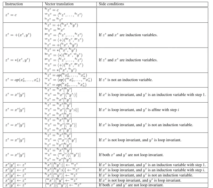
This initial step defines vector and last value variables for each base induction variable of the loop, as well as basis and promoted variables. The translation of each instruction then proceeds com-positionally, with the translated version of each instruction making use of the vector and last value variables produced by the trans-lation of all of the previous instructions. In addition, each induc-tion variable makes use of the previously defined basis variables to produce its own vector, last value, basis, and promoted variables directly. The complete definition of this translation is given in Fig-ure 2.

Adjusting the exit test of the loop is again straightforward using the step information. The desired new exit test must check whether

Instruction Vector translation Side conditions zs_=c fv_zs_=c vv_zv_=hfv_zs_{, . . . ,}fv_zs_i lv_zs₌fv_zs zs_{= +(x}s_{, y}s₎ fv_zs_{= +(}fv_xs_,fv_ys₎ bv_zv₌bv_xv pv_zv_=hfv_zs_{, . . . ,}fv_zs_i vv_zv_=h+i(bv_zv_,pv_zv₎ lv_zs_{= +(}lv_xs_,fv_ys₎ Ifzs andxs

are induction variables.

zs_=∗(xs_{, y}s₎ fv_zs_=∗(fv_xs_,fv_ys₎ bv_zv_=h∗i(bv_xv_,vv_yv₎ pv_zv_=hfv_zs_{, . . . ,}fv_zs_i vv_zv_=h+i(bv_zv_,pv_zv₎ lv_zs_=∗(lv_xs_,fv_ys₎

Ifzs_andxs_{are induction variables.}

zs_=op(xs 0, . . . , xsn) fv_zs₌ op(fv_xs 0, . . . ,fvxsn) vv_zv_=h opi(vv_xv 0, . . . ,vvxvn) lv_zs₌ op(lv_xs 0, . . . ,lvxsn)

Ifzs_{is not an induction variable.}

zs_=xs_[ys_]

fv_zs₌fv_xs_[fv_ys_]

vv_zv₌fv_xs_[hfv_ys_:i]

lv_zs₌fv_xs_[lv_ys_]

Ifxs_{is loop invariant, andy}s_{is an induction variable with step 1.}

zs_=xs_[ys_]

fv_zs₌fv_xs_[fv_ys_]

vv_zv₌fv_xs_[hfv_ys_:ii]

lv_zs₌fv_xs_[lv_ys_]

Ifxs_{is loop invariant, andy}s_{is affine with stepi}

zs_=xs_[ys_]

fv_zs₌fv_xs_[fv_ys_]

vv_zv₌fv_xs_[hvv_yv_i]

lv_zs₌fv_xs_[lv_ys_]

Ifxs_{is loop invariant, andy}s_{is not an induction variable.}

zs_=xs_[ys_]

fv_zs₌fv_xs_[fv_ys_]

vv_zv_=hvv_xv_i[fv_ys_]

lv_zs₌lv_xs_[fv_ys_]

Ifxs

is not loop invariant, andys

is loop invariant.

zs_=xs_[ys_]

fv_zs₌fv_xs_[fv_ys_]

vv_zv_=hvv_xv_i[hvv_yv_i]

lv_zs₌lv_xs_[lv_ys_]

If bothxs_andys_{are not loop invariant.}

xs_[ys_]←zs fv_xs_[hfv_ys_:i]←vv_zv _Ifxs_{is loop invariant, andy}s_{is an induction variable with step 1.}

xs_[ys_]←zs fv_xs_[hfv_ys_:ii]←vv_zv _Ifxs_{is loop invariant, andy}s_{is an induction variable with stepi.}

xs_[ys_]←zs fv_xs_[hvv_yv_i]←vv_zv _Ifxs_{is loop invariant, andy}s_{is not an induction variable.}

xs_[ys_]←zs _hvv_xv_i[fv_ys_]←vv_zv _Ifxs_{is not loop invariant, andy}s_{is loop invariant.}

xs_[ys_]←zs _hvv_xv_i[hvv_yv_i]←vv_zv _{If bothx}s_andys_{are not loop invariant.} Figure 2. Vector Block Instruction Translation

is _{< l}s_{would succeed for at least eight more iterations. Sincei}s

is an induction variable, lettingsbe its step, it increases byson each iteration. Thus the value ofis_{on the next eight iterations will}

belv_is_{+ 0∗s, . . . ,}lv_is_{+ 7∗s. These will all be less thanl}s_{if the}

last of them is less thanls_{(recall thatl}s_{is loop invariant). Thus the}

desired new exit condition islv_is_{+ 7∗s < l}s_.

Putting this all together the vector loop will be as follows, where

i′s_{is a fresh variable:}

Lvec(fv_is

0, . . . ,fvisn):

Instructions for base induction variables TransformedI0, . . . ,Im

i′s_{= +(}lv_is_,7∗s) if(i′s _{< l}s_)goto

Lvec(lv_is

01, . . . ,lvisn1)

else gotoLcheck()

Note that the back edge targets the vector loop, the exit edge targets the cleanup check, and the last values of the base induction variables are passed on the back edge.

4.4.3 On the subject of overflow

For the most part, the vectorization transformation here is careful to only compute the same values computed in the original program. Generating entry and exit tests violate this property. As mentioned in Section 4.4.1, the compiler can check statically that overflow does not occur when computing constants for the initial entry test. For the exit test, it is sufficient to check before entry to the vector loop thatls _{< MI−7∗swhere MI is the largest representable}

integer ands is the step ofis_{. For signed types, this check must}

be adjusted in the obvious way when loop bounds or steps are negative. In all cases, if the checks fail then the original scalar loop is used to perform the calculation using the original code.

4.4.4 Cleanup check

The cleanup check is responsible for determining if scalar iterations remain to be performed after the vector loop has exited. This is done simply by performing the original loop exit test. Scalar iterations remain to be performed exactly whenlvis_{< l}s

, wherelvis

is the last value foris

Entry test Vector loop Cleanup check Optimized result L0(): as₌ new[ls_] is 0= 0 fv_as_=as vv_av_=has_{, . . . , a}s_i lv_as_=as fv_bs_=bs vv_bv_=hbs_{, . . . , b}s_i lv_bs_=bs fv_cs_=cs vv_cv_=hcs_{, . . . , c}s_i lv_cs_=cs fv_ls_=ls vv_lv_=hls_{, . . . , l}s_i lv_ls_=ls iis_{= 6∗1 + 1} if(iis _{< l}s₎ goto L2(is 0) else goto L1(is 0) L2(fv_is_): bv_iv_{=h0∗1, . . . ,7∗1i} pv_iv_=hfv_is_{, . . . ,}fv_is_i vv_iv_=h+i(bv_iv_,pv_iv₎ lv_is_{= +(}fv_is_,7∗1) fv_xs₌fv_bs_[fv_is_] vv_xv₌fv_bs_[hfv_is_:i] lv_xs₌fv_bs_[lv_is_] fv_ys₌fv_cs_[fv_is_] vv_yv₌fv_cs_[hfv_is_:i] lv_ys₌fv_cs_[lv_is_] fv_zs_{= +(}fv_xs_,fv_ys₎ vv_zv_=h+i(vv_xv_,vv_yv₎ lv_zs_{= +(}lv_xs_,lv_ys₎ fv_as_[hfv_is_:i]←vv_zv fv_is 1= +(fvis,1) bv_iv 1=bviv pv_iv 1=hfvis1, . . . ,fvis1i vv_iv 1 =h+i(bviv1,pviv1) lv_is 1= +(lvis,1) i′s 1 = +(lvis1,7∗1) if(i′s 1 < ls)goto L 2 (lv_is 1)

else goto Lcheck₍₎

Lcheck(): is 2= +( fv_is_,7∗1) is 3= +(is2,1) if(is 3 < ls)goto L 1 (is 3)

else goto Lexit(is

3) L0(): as₌ new[ls_] is 0 = 0 iis_{= 7} if(iis _{< l}s₎ goto L2(is 0) else goto L1 (is 0) L2(fv_is_): lv_is_{= +(}fv_is_,7) vv_xv_=bs_[hfv_is_:i] vv_yv_=cs_[hfv_is_:i] vv_zv_=h+i(vv_xv_,vv_yv₎ as_[hfv_is_:i]←vv_zv lv_is 1= +(lvis,1) i′s 1 = +(lvis1,7) if(i′s 1 < ls)goto L 2 (lv_is 1)

else goto Lcheck()

Lcheck(): is 2 = +(fvis,7) is 3 = +(is2,1) if(is 3 < ls)goto L 1 (is 3)

else goto Lexit(is

3)

Figure 3. Vectorized version of Example 1

value ofis_{from the last completed iteration). Since the vector loop}

dominates the cleanup check, all its entry variables and variables it defines are in scope, so the cleanup check could be formed as:

Lcheck():

if(lv_is _{< l}s_)goto

L(lv_is

01, . . . ,lvisn1)

else gotoLexit(lv_xs

0, . . . ,lvxsp)

Note that the last values of the base induction variables are passed to the scalar loop and the last values of the live-out variables (xs

0, . . . , xsp) are passed to the exit label.

However, instead of using the last values computed in the vec-tor loop, it is better to recompute them in order to avoid introducing data dependencies that may keep instructions live in the loop which could otherwise be eliminated. This turns out to be straightforward: the portion of the translation in Figure 2 that computes last values can simply be repeated. This results in a complete calculation of all of the last values, includinglv_is_{. While most of these}

instruc-tions will turn out to be unnecessary, a single pass of dead code elimination is sufficient to eliminate them.

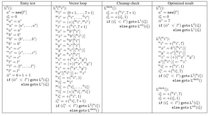
4.5 Transformed example

The actual process of producing SIMD vector versions of loops seems at first quite ad hoc and difficult to do cleanly, but turns out to be amenable to a simple and straightforward translation which systematically produces vector versions of scalar instructions, rely-ing on orthogonal optimizations to clean up unnecessary generated code. To illustrate the results of this process, Figure 3 shows the results of applying the algorithm to Example 1. First note that the base induction variables are justis

of step 1, and the only other induction variable is is

1 also of step 1. The variables as, bs,cs,

andls _{are used in the loop but not defined by it. BlockL}0

is the preheader for the loop. We first transform the preheader to define variables used by but not defined by the loop and to do the entry test. This results in Figure 3 under the header “Entry test”. Next

we generate the instructions for the base induction variable, trans-formed instructions of the loop, and adjusted exit condition to form the vector loop. The result of this appears under the header “Vec-tor loop”. Finally we form the cleanup check by regenerating the last-value computations and using the original loop-exit condition. For simplicity we just show enough instructions to compute the last value ofis

1, the only needed last value. This block appears under the

header “Cleanup check”.

This code, as expected, is terribly verbose. However, by apply-ing copy propagation followed by dead-code elimination, the ex-traneous parts disappear, yielding the code shown under the header “Optimized result”. By applying common sub-expression elimina-tion this code can be further improved by eliminating the calcula-tion ofis

2in favor oflvis, andis3in favor oflvis1. Finally, simplifying

the chained arithmetic expressions yields the same vectorized loop as derived by the initial ad hoc vectorization shown in Section 4.3.

4.6 Reductions

The SIMD vectorization process defined so far primarily applies to loops which serve to create new arrays. An additional idiom that is important to handle in vectorization is that of loops which serve (in total or in part) to compute a reduction using a binary operator. That is, instead of, or in addition to, initializing a new array, each itera-tion of the loop accumulates a value into an accumulator parameter as a function of the value from the last iteration. For example, the innermost dot product of a matrix multiply routine generally takes the form of a reduction.

Adding support for reductions to the vectorization transforma-tion is not difficult. In the same manner that we identify certain variables as induction variables and treat them specially, we iden-tify variables that fit the pattern of reductions and add additional cases to the vectorization transformation to handle them differently. Specifically, we say that a variablexs

is a reduction variable if it is a parameter to the loop that is not an induction variable, and