Contents lists available atScienceDirect
Artificial Intelligence
www.elsevier.com/locate/artint
AND/OR Branch-and-Bound search for combinatorial optimization
in graphical models
Radu Marinescu
a,
∗
,
1, Rina Dechter
b aCork Constraint Computation Centre, University College Cork, IrelandbDonald Bren School of Information and Computer Science, University of California, Irvine, CA 92697, USA
a r t i c l e
i n f o
a b s t r a c t
Article history: Received 12 April 2008
Received in revised form 1 July 2009 Accepted 10 July 2009
Available online 21 July 2009 Keywords: Search AND/OR search Decomposition Graphical models Bayesian networks Constraint networks Constraint optimization
This is the first of two papers presenting and evaluating the power of a new framework for combinatorial optimization in graphical models, based on AND/OR search spaces. We introduce a new generation of depth-first Branch-and-Bound algorithms that explore the AND/OR search tree using static and dynamic variable orderings. The virtue of the AND/OR representation of the search space is that its size may be far smaller than that of a traditional OR representation, which can translate into significant time savings for search algorithms. The focus of this paper is on linear space search which explores the AND/OR search tree. In the second paper we explore memory intensive AND/OR search algorithms. In conjunction with the AND/OR search space we investigate the power of the mini-bucket heuristics in both static and dynamic setups. We focus on two most common optimization problems in graphical models: finding the Most Probable Explanation in Bayesian networks and solving Weighted CSPs. In extensive empirical evaluations we demonstrate that the new AND/OR Branch-and-Bound approach improves considerably over the traditional OR search strategy and show how various variable ordering schemes impact the performance of the AND/OR search scheme.
©2009 Elsevier B.V. All rights reserved.
1. Introduction
Graphical models such as Bayesian networks or constraint networks are a widely used representation framework for reasoning with probabilistic and deterministic information. These models use graphs to capture conditional independencies between variables, allowing a concise representation of the knowledge as well as efficient graph-based query processing algorithms. Optimization problems such as finding the most likely state of a Bayesian network or finding a solution that violates the least number of constraints can be defined within this framework and they are typically tackled with either inferenceorsearchalgorithms.
Inference-based algorithms (e.g., Variable Elimination, Tree Clustering) were always known to be good at exploiting the independencies captured by the underlying graphical model. They provide worst case time guarantees exponential in the treewidth of the underlying graph. Unfortunately, any method that is time-exponential in the treewidth is also space exponential in the treewidth or separator width, therefore not practical for models with large treewidth.
Search-based algorithms (e.g., depth-first Branch-and-Bound search) traverse the model’s search space where each path represents a partial or full solution. The linear structure of such traditional search spaces does not retain the independen-cies represented in the underlying graphical models and, therefore, search-based algorithms may not be nearly as effective
*
Corresponding author.E-mail addresses:[email protected](R. Marinescu),[email protected](R. Dechter). 1 This work was done while at the University of California, Irvine.
0004-3702/$ – see front matter ©2009 Elsevier B.V. All rights reserved. doi:10.1016/j.artint.2009.07.003
as inference-based algorithms in using this information. Moreover, these methods do not accommodate informative perfor-mance guarantees. This situation has changed in the past few years with the introduction of AND/OR search algorithms for graphical models. In addition, search methods require only an implicit, generative, specification of the functional rela-tionships (that may be given in a procedural or functional form) while inference schemes often rely on an explicit tabular representation over the (discrete) variables. For these reasons, search-based algorithms are usually the preferred choice for models with large treewidth and with implicit representation.
The AND/OR search space for graphical models [1] is a new framework that is sensitive to the independencies in the model, often resulting in exponentially reduced complexities. It is guided by apseudo tree[2,3] that captures independencies in the graphical model, resulting in a search space exponential in the depth of the pseudo tree, rather than in the number of variables.
In this paper we present a new generation of AND/OR Branch-and-Bound algorithms (
AOBB
) that explore the AND/OR search tree in a depth-first manner for solving optimization problems in graphical models. As in traditional Branch-and-Bound search, the efficiency of these algorithms depends heavily also on their guiding heuristic function. A class of partitioning-based heuristic functions, based on the Mini-Bucket approximation [4] and known asstatic mini-bucket heuristics was shown to be powerful for optimization problems [5] in the context of the traditional OR search spaces. The Mini-Bucket algorithm provides a scheme for extracting heuristic information from the functional specification of the graphical model and is applicable to any graphical model. The accuracy of the Mini-Bucket algorithm is controlled by a bounding parameter, calledi-bound, which allows varying degrees of heuristics accuracy and results in a spectrum of search algorithms that can trade off heuristic strength and search [5]. We show here how the pre-computed mini-bucket heuristic as well as any other heuristic information can be incorporated into AND/OR search. We also introducedynamic mini-bucket heuristics, which are computed dynamically at each node of the search tree.Since variable orderings can influence dramatically the search performance, we also introduce a collection of dynamic AND/OR Branch-and-Bound algorithms that combine AND/OR decomposition with dynamic variable orderings.
We apply the depth-first AND/OR Branch-and-Bound approach to two common optimization problems in graphical mod-els: finding the Most Probable Explanation (MPE) in Bayesian networks [6] and solving Weighted Constraint Satisfaction Problems (WCSP) [7]. Our results show conclusively on various benchmark problems that the new depth-first AND/OR Branch-and-Bound algorithms improve dramatically over traditional ones exploring the OR search space, especially when the heuristic estimates are inaccurate and the algorithms rely primarily on search.
Following preliminary notations and definitions (Section 2), Sections 3, 4 and 5 provide background on graphical models, on the classic OR Branch-and-Bound approach, and on the AND/OR representation of the search space. Section 6 presents our new depth-first AND/OR Branch-and-Bound algorithm. Section 7 presents several general purpose heuristic functions that can guide the search focusing on the mini-bucket heuristics. Section 8 describes its extension with dynamic variable ordering heuristics. Section 9 shows the empirical evaluation, Section 10 overviews related work and Section 11 provides a summary and concluding remarks.
2. Preliminaries
2.1. Notations
A reasoning problem is defined in terms of a set of variables taking values on finite domains and a set of func-tions defined over these variables. We denote variables by uppercase letters (e.g., X
,
Y,
Z, . . .
), sets of variables by bold faced uppercase letters (e.g., X,
Y,
Z, . . .
) and values of variables by lower case letters (e.g., x,
y,
z, . . .
). An assignment(
X1=
x1, . . . ,
Xn=
xn)
can be abbreviated as x=
(
X1,
x1, . . . ,
Xn,
xn)
orx=
(
x1, . . . ,
xn)
. For a subset of variables Y, DYdenotes the Cartesian product of the domains of variables inY.xYandx
[
Y]
are both used as the projection ofx=
(
x1, . . . ,
xn)
over a subsetY. We denote functions by letters f,
h,
g etc., and the scope (set of arguments) of a function f byscope(
f)
.2.2. Graph concepts
Definition 1 (directed, undirected graphs). Adirected graphis defined by a pair G
= {
V,
E}
, where V= {
X1, . . . ,
Xn}
is a set of vertices (nodes), andE= {
(
Xi,
Xj)
|
Xi,
Xj∈
V}
is a set of edges (arcs). If(
Xi,
Xj)
∈
E, we say that Xi points toXj. The degree of a vertex is the number of incident arcs to it. For each vertex Xi,pa(
Xi)
orpai, is the set of vertices pointing to Xi inG, while the set of child vertices of Xi, denotedch(
Xi)
, comprises the variables that Xi points to. The family of Xi, denoted Fi, includes Xi and its parent vertices. A directed graph is acyclic if it has no directed cycles. Anundirectedgraph is defined similarly to a directed graph, but there is no directionality associated with the edges.Definition 2 (induced width). An ordered graphis a pair
(
G,
d)
where G is an undirected graph, andd=
X1, . . . ,
Xn is an ordering of the nodes. Thewidth of a nodeis the number of the node’s neighbors that precede it in the ordering. Thewidth of an ordering d is the maximum width over all nodes. Theinduced width of an ordered graph, denoted by w∗(
d)
, is the width of the induced ordered graph obtained as follows: nodes are processed from last to first; when node Xiis processed, all its preceding neighbors are connected. Theinduced widthof a graph, denoted byw∗, is the minimal induced width over all its orderings.Definition 3(hypergraph).Ahypergraphis a pairH
=
(
X,
S)
, whereS= {
S1, . . . ,
St}
is a set of subsets ofX, called hyperedges.Definition 4(tree decomposition).Atree decomposition of a hypergraph H
=
(
X,
S)
, is a tree T=
(
V,
E)
, whereVis a set of nodes, also called “clusters”, andE is a set of edges, together with a labeling functionχ
that associates with each vertex v∈
Va setχ
(
v)
⊆
Xsatisfying:(1) For each Si
∈
Sthere exists a vertex v∈
Vsuch thatSi⊆
χ
(
v)
;(2) For each Xi
∈
X, the set{
v∈
V|
Xi∈
χ
(
v)
}
induces a connected subtree ofT (running intersection property).Definition 5 (treewidth, pathwidth). The width of a tree decomposition of a hypergraph is the size of the largest cluster minus 1 (i.e., maxv
|
χ
(
v)
−
1|
). Thetreewidthof a hypergraph is the minimum width along all possible tree decompositions. Thepathwidthis the treewidth over the restricted class of chain decompositions.2.3. AND/OR search spaces
An AND/OR state space representation of a problem is a 4-tuple
S,
O,
Sg,
s0 [8]. S is a set of states which can be either OR or AND states (the OR states represent alternative ways for solving the problem while the AND states often represent problem decomposition into subproblems, all of which need to be solved). O is a set of operators. An OR operator transforms an OR state into another state, and an AND operator transforms an AND state into a set of states. There is a set of goal states Sg⊆
Sand a start nodes0∈
S.The AND/OR state space model induces an explicit AND/OR search graph. Each state is a node and child nodes are obtained by applicable AND or OR operators. The search graph includes astartnode. The terminal nodes (having no children) are labeled asSolvedorUnsolved.
Asolution treeof an AND/OR search graphG is a subtree which: (1) contains the start nodes0; (2) ifnin the tree is an OR node then it contains one of its child nodes in G, and ifnis an AND node it contains all its children in G; (3) all its terminal nodes areSolved.
3. Graphical models
Graphical models include constraint networks defined by relations of allowed tuples, directed or undirected probabilistic networks and cost networks defined by cost functions. Each graphical model comes with its specific optimization queries such as finding a solution of a constraint network that violates the least number of constraints, finding the most probable assignment given some evidence, posed over probabilistic networks, or finding the optimal solution for cost networks.
In general, a graphical model is defined by a collection of functionsF, over a set of variablesX, conveying probabilistic or deterministic information, whose structure is captured by a graph.
Definition 6(graphical model).Agraphical model
R
is defined by a 4-tupleR
=
X,
D,
F,
⊗
, where: (1) X= {
X1, . . . ,
Xn}
is a set of variables;(2) D
= {
D1, . . . ,
Dn}
is the set of their respective finite domains of values;(3) F
= {
f1, . . . ,
fr}
is a set of real-valued functions, each defined over a subset of variablesSi⊆
X(i.e., the scope); (4) ifi∈ {
ifi,
ifi
}
is a combination operator.The graphical model represents the combination of all its functions:
ri=1fi.Definition 7(cost of a full and partial assignment).Given a graphical model
R
, the cost of a full assignmentx=
(
x1, . . . ,
xn)
is defined by:c
(
x)
=
f∈Ff
xscope(
f)
.
Given a subset of variablesY
⊆
X, the cost of a partial assignment yis the combination of all the functions whose scopes are included inY, namely FY, evaluated at the assigned values. Namely,c(
y)
=
f∈FY f(
y[
scope(
f)
]
)
. We will often abuse notation writingc(
y)
=
f∈FY f(
y)
instead.Definition 8(primal graph).Theprimal graphof a graphical model has the variables as its nodes and an edge connects any two variables that appear in the scope of the same function.
There are various queries (tasks) that can be posed over graphical models. We refer to all asautomated reasoning problems. In general, an optimization task is a reasoning problem defined as a function from a graphical model to a set of elements, most commonly, the real numbers.
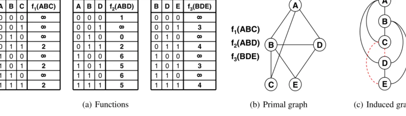
Fig. 1.A WCSP instance with cost functions f1(A,B,C), f2(A,B,D)and f3(B,D,E).
Definition 9 (constraint optimization problem). A constraint optimization problem(COP) is a pair
P
=
R
,
⇓
X, whereR
=
X,
D,
F,
⊗
is a graphical model. If S is the scope of function f∈
F then⇓
S f∈ {
maxS f,
minS f}
and the optimization problem is to compute⇓
Xri=1 fi.The min/max (
⇓
) operator is sometimes called aneliminationoperator because it removes the arguments inS from the input functions’ scopes.We next overview briefly two popular graphical models of constraint networks and belief networks, which will be the primary focus of this paper. For a detailed description of these models we refer the reader to [1,9].
A constraint network
R
=
X,
D,
C has a set of constraints C= {
C1, . . . ,
Cr}
as its functions. Each constraint is a pair Ci=
(
Si,
Ri)
, where Si⊆
X is the scope of the relation Ri defined over Si, denoting the allowed combinations of values. The primal graph of a constraint network is called a constraint graph. The Constraint Satisfaction Problem (CSP) seeks to determine if a constraint network has a solution, and if so, to find one.An immediate extension of constraint networks are cost networks where the set of functions are real-valued functions, the combination and elimination operators aresummationandminimization, respectively, and the primary constraint opti-mization task is to find a solution having minimum cost. A special class of constraint optiopti-mization problems that has gained attention in recent years is the Weighted Constraint Satisfaction Problem (WCSP). WCSP extends the classical CSP formalism withsoft constraints which are represented asinteger-valuedcost functions. In a WCSP
W
=
X,
D,
Feach function fi∈
F assigns “0” (no penalty) to allowed tuples and a positive integer penalty to forbidden tuples. The optimization problem is to find a value assignment to the variables with minimum penalty. As a reasoning problem, solving a WCSP is to find⇓
Xri=1=
minXri=1fi.Example 1. Fig. 1 shows an example of a WCSP instance with bi-valued variables. The cost functions are given in Fig. 1(a). The value
∞
indicates an inconsistent tuple. Figs. 1(b) and 1(c) depict the primal and the induced graph along the ordering d=
(
A,
B,
C,
D,
E,
F)
, respectively. The induced graph is obtained by adding the dotted-arcs. It can be shown that the minimal cost solution is 5 and corresponds to the assignment(
A=
0,
B=
1,
C=
1,
D=
0,
E=
1)
.Abelief network
B
=
X,
D,
P is defined over a directed acyclic graphG=
(
X,
E)
and its functions Pi∈
P denote condi-tional probability tables (CPTs), Pi=
P(
Xi|
pai)
, where pai is the set ofparent nodes pointing to Xiin G. A belief network represents a joint probability distribution over X, P(
X1, . . . ,
Xn)
=
ni=1P
(
Xi|
pai)
. When formulated as a graphical model, the scopes of the functions in Pare determined by the directed acyclic graph G: each function fi ranges over variable Xi and its parents in G. The combination operator is multiplication, namelyj=
j. The primal graph of a belief network is called amoral graph. It connects any two variables appearing in the same probability table.A common optimization task is themost probable explanation(MPE) task. It calls for finding a complete assignment which agrees with the evidenceein the network, whereean instantiated subset of variables, and which has the highest probability among such assignments, namely to find an assignment
(
xo1, . . . ,
xno)
such that: P(
xo1, . . . ,
xon)
=
maxx1,...,xn ni=1P
(
xi,
e|
xpai)
.As a reasoning problem, the MPE task is to find
⇓
X ri=1fi
=
maxX n i=1Pi.Overview of previous work on WCSP and MPE.We will mention related work separately for WCSP and MPE. Clearly, both tasks are NP-hard. A number of complete and incomplete algorithms have been developed for WCSP. Stochastic Local Search (SLS) algorithms, such as GSAT [10,11], developed for Boolean Satisfiability and Constraint Satisfaction can be directly ap-plied to WCSP [12]. SLS algorithms cannot guarantee an optimal solution, but they have been successful in practice on many classes of SAT and CSP problems. A number of search-based complete algorithms, using partial forward checking [13] for heuristic computation, have been developed [14,15]. The Branch-and-Bound algorithm proposed by [5] uses bounded mini-bucket inference to compute the guiding heuristic function. More recently, [16–18] introduced a family of depth-first Branch-and-Bound algorithms that maintain various levels of directional soft arc-consistency.
Complete algorithms for MPE used in the past either the cycle cutset technique (also called conditioning) [6], the join-tree clustering technique [19,20], or the bucket elimination scheme [21]. These methods work well only if the network is sparse enough. The algorithms based on cutset conditioning have time complexity exponential in the cutset size but require only linear space, whereas join-tree clustering and bucket elimination algorithms are both time and space exponential in the cluster size that equals the induced width (or treewidth) of the network’s moral graph. Following Pearl’s stochastic simulation algorithms [6], the suitability of Stochastic Local Search (SLS) algorithms for MPE was studied in the context of medical diagnosis applications [22] and more recently in [23–25]. Best-First search algorithms were proposed [26] as well as algorithms based on linear programming [27]. Some extensions are also available for the task of finding thekmost-likely explanations [28,29]. We recently introduced in [5,30] a collection of depth-first Branch-and-Bound algorithms that use bounded inference, in particular the Mini-Bucket approximation [4], for computing the guiding heuristic function.
In the next section we present inference and search approaches on which we build in this paper. 4. Search and inference for combinatorial optimization
4.1. Bucket and mini-bucket elimination
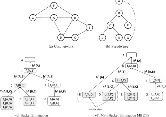
Bucket Elimination(BE) is a unifying framework for inference (e.g., dynamic programming) applicable to probabilistic and deterministic reasoning [21]. Given an optimization problem, namely a collection of cost functions, and given a variable orderingd, the algorithm partitions the functions into buckets, each associated with a single variable. A function is placed in the bucket of its argument that appears latest in the ordering. The algorithm has two phases. During the first, top-down phase, it processes each bucket, from last to first by a variable elimination procedure that computes a new function which is placed in a lower bucket. The variable elimination procedure computes the combination of all functions and eliminates the bucket’s variable. During the second, bottom-up phase, the algorithm constructs a solution by assigning a value to each variable along the ordering, consulting the functions created during the top-down phase. The complexity of the algorithm is time and space O
(
exp(
w∗))
, wherew∗is the induced width of the primal graph along the orderingd[21].BE can be viewed as message passing from leaves to root along a bucket tree [9]. Let
{
B(
X1), . . . ,
B(
Xn)
}
denote a set of buckets, one for each variable, along an orderingd=
(
X1, . . . ,
Xn)
. A bucket treehas buckets as its nodes. Bucket B(
X)
is connected to bucket B(
Y)
if the function generated in bucket B(
X)
by BE is placed in B(
Y)
. The variables of B(
X)
, are those appearing in the scopes of any of its new and old functions.Mini-Bucket Elimination (MBE) is an approximation of bucket elimination. It is designed to avoid the space and time problem of full bucket elimination by partitioning large buckets into smaller subsets, calledmini-buckets, each containing at most i (called i-bound) distinct variables. The mini-buckets are then processed separately [4]. The algorithm outputs not only a lower bound (resp. an upper bound for maximization problems) on the cost of the optimal solution and an assignment, but also the collection of theaugmented buckets which contain both the original as well as the intermediate functions generated by the algorithm. The complexity of the algorithm, which is parameterized by thei-bound, is time and space O
(
exp(
i))
where i<
n [4]. It can be viewed as solving by bucket elimination a simplified problem that is sparser [5,31]. When the i-bound is large enough (i.e., iw∗), the Mini-Bucket algorithm coincides with full BE on the original problem.4.2. Branch-and-Bound search with mini-bucket heuristics
Most exact search algorithms for solving optimization problems in graphical models follow a Branch-and-Bound schema [32]. This algorithm performs a depth-first traversal of the search tree defined by the problem, where internal nodes represent partial assignments and leaf nodes stand for complete ones. Throughout the search, the algorithm main-tains a global bound on the cost of the optimal solution, which corresponds to the cost of the best full variable instantiation found thus far. At each node, the algorithm computes a heuristic estimate of the best solution extending the current partial assignment and prunes the respective subtree if the heuristic estimate is not better than the current global bound (that is – not greater for maximization problems, not smaller for minimization problems). The algorithm requires only a limited amount of memory and can be used as an anytime scheme, namely whenever interrupted, Branch-and-Bound outputs the best solution found so far.
The effectiveness of Branch-and-Bound depends on the quality of the heuristic function. We next describe briefly a general scheme for generating heuristic estimates based on the Mini-Bucket approximation. This scheme is parameterized by the Mini-Bucket i-bound, thus allowing for a controllable trade-off between pre-processing (for heuristics generation) and search [5].
Definition 10(mini-bucket heuristic evaluation function [5]).Given an ordered set of augmented buckets
{
B(
X1), . . . ,
B(
Xp), . . . ,
B(
Xn)
}
generated by the Mini-Bucket algorithm MBE(
i)
along the orderingd=
(
X1, . . . ,
Xp, . . . ,
Xn)
, and given a partial as-signment¯
xp=
(
x1, . . . ,
xp)
, the heuristic evaluation function f(
x¯
p)
=
g(
¯
xp)
+
h(
x¯
p)
is defined follows:(1) g
(
x¯
p)
=
(
fi∈B(X1...Xp)fi
)(
¯
xp)
is thecombinationof all the input functions that are fully instantiated along the current path, where B(
X1. . .
Xp)
denotes the buckets B(
X1)
through B(
Xp)
in the orderingd;(2) The mini-bucket heuristic function h
(
¯
xp)
is defined as the combination of all the intermediate functions hkj, h(
x¯
p)
=
(
hkj∈B(X1...Xp)h
k j
)(
¯
xp
)
, that satisfy the following properties:•
They are generated in bucketsB(
Xp+1)
through B(
Xn)
,•
They reside in buckets B(
X1)
through B(
Xp)
.Kask and Dechter showed [5] that for any partial assignment
¯
xp=
(
x1, . . . ,
xp)
of the first p variables in the ordering, the evaluation function f(
¯
xp)
=
g(
x¯
p)
+
h(
x¯
p)
isadmissibleandmonotonic[8].Branch-and-Boundguided by theMini-Bucket heuristicsis denoted by BBMB(i). The algorithm was introduced for a static variable ordering and has a space complexity dominated by the pre-processing step which is exponential in thei-bound [5]. BBMB(i) was evaluated extensively for probabilistic and deterministic optimization tasks. The results showed conclusively that the scheme overcomes partially the memory explosion of bucket elimination allowing a gradual trade-off of space for time, and of time for accuracy when used as an anytime scheme.
Subsequently, [30,33] explored the feasibility of generating partition-based heuristics during search, rather than in a pre-processing manner. This allows dynamic variable and value ordering, a feature that can have tremendous impact on search. The dynamic generation of these heuristics is facilitated by Mini-Bucket-Tree Elimination, MBTE(i), a partition-based approximation defined over cluster-trees [33]. MBTE(i) outputs multiple (lower or upper) bounds for each possible variable and value extension at once, which is much faster than running MBE(i)ntimes, once for each variable.
The resultingBranch-and-Bound with Mini-Bucket-Tree heuristics[30,33], called BBBT(i), applies the MBTE(i) heuristic com-putation at each node of the search tree. Clearly, the algorithm has a higher time overhead compared with BBMB(i) for the samei-bound, which computes the mini-buckets once. It is exponential in thei-bound multiplied by the number of nodes visited, but it can prune the search space much more effectively. Experimental results on probabilistic and deterministic graphical models showed that the power of BBBT(i) is more pronounced over BBMB(i) only at relatively small i-bounds. This quality is important because smalli-bounds imply restricted space.
5. AND/OR search trees for graphical models
In this section we overview the AND/OR search space for graphical models [1,8], which forms the core of our work in this paper. For simplicity and without loss of generality we consider in the remainder of the paper an optimization problem
P
=
R
,
minover a graphical modelR
=
X,
D,
F,
for which the combination and elimination operators aresummation andminimization, respectively.As noted in Section 4, the usual way to do search in graphical models is to instantiate variables in turn, following a static/dynamic variable ordering. In the simplest case this process defines a search tree (called here OR search tree), whose state nodes represent partial variable assignments. In order to capture the independence structure of the underlying graphical model it was recently extended by AND nodes, yielding the AND/OR search space for graphical models [1]. The AND/OR search space is defined using apseudo tree[2,3].
Definition 11 (pseudo tree, extended graph).Given an undirected graph G
=
(
V,
E)
, a directed rooted treeT
=
(
V,
E)
defined on all its nodes is called pseudo treeif any arc ofG which is not included inE is a back-arc, namely it connects a node to an ancestor inT
. The arcs inEmay not all be included inE. Given a pseudo treeT
ofG, theextended graphofG relative toT
is defined asGT=
(
V,
E∪
E)
.We next define the notion of AND/OR search tree for a graphical model.
Definition 12(AND/OR search tree [1]).Given a graphical model
R
, its primal graphG and a backbone pseudo treeT
ofG, the associated AND/OR search tree, denoted ST(
R
)
, has alternating levels of AND and OR nodes. The OR nodes are labeled Xiand correspond to the variables. The AND nodes are labeledXi,
xi(or simplyxi) and correspond to value assignments in the domains of the variables. The structure of the AND/OR search tree is based on the underlying backbone pseudo treeT
. The root of the AND/OR search tree is an OR node labeled with the root ofT
. The children of an AND nodeXi,
xi are OR nodes labeled with the children of variable XiinT
. A path from the root of the search tree ST(
R
)
to a nodenis denoted byπn
. Ifn is labeled Xi or xi the path will be denotedπn
(
Xi)
orπn
(
xi)
, respectively. The assignment sequence along pathπn
, denotedasgn(
πn
)
, is the set of value assignments associated with the AND nodes alongπn
.Semantically, the OR states in the AND/OR search tree represent alternative ways of solving a problem, whereas the AND states represent problem decomposition into independent subproblems, conditioned on the assignment above them, all of which need to be solved.
Following the general definition of a solution tree for AND/OR search spaces [8] we have here that:
Definition 13 (solution tree). A solution tree of an AND/OR search tree ST
(
R
)
is an AND/OR subtree T such that: (i) it contains the root of ST(
R
)
, s; (ii) if a non-terminal AND noden∈
ST(
R
)
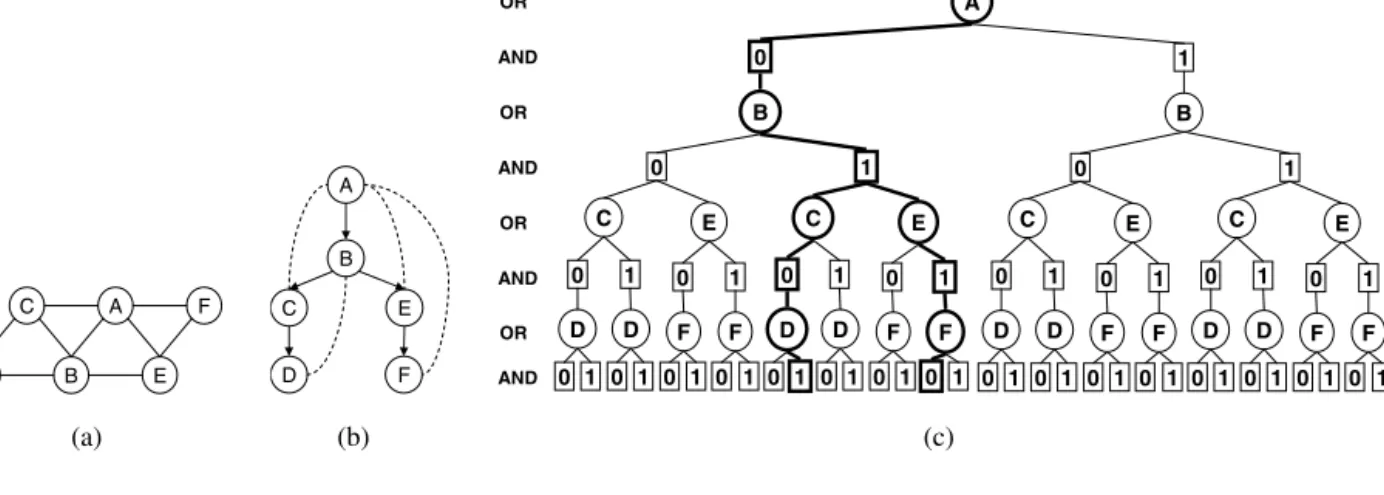
is inT then all of its children are inT; (iii) ifFig. 2.AND/OR search spaces for graphical models.
a non-terminal OR noden
∈
ST(
R
)
is in T then exactly one of its children is in T; (iv) all its leaf (terminal) nodes are consistent.Example 2.Fig. 2(a) shows the primal graph of cost network with 6 bi-valued variables A,B,C, D, E and F, and 9 binary cost functions. Fig. 2(b) displays a pseudo tree together with the back-arcs (dotted lines). Fig. 2(c) shows the AND/OR search tree based on the pseudo tree. A solution tree is highlighted. Notice that once variablesA andBare instantiated, the search space below the AND node labeled
B,
0decomposes into two independent subproblems, one that is rooted atC and one that is rooted at E, respectively.The virtue of an AND/OR search tree representation is that its size may be far smaller than the traditional OR search tree. It was shown that the AND/OR search tree represents all solutions and is therefore sound. Its size is controlled by some graph parameters, as follows:
Theorem 1(size of AND/OR search trees [1]). Given a graphical model
R
and a backbone pseudo treeT
, the size of its AND/OR search tree ST(
R
)
is O(
l·
km)
where m is the depth of the pseudo tree, l bounds its number of leaves, and k bounds the domain size. Moreover, ifR
has treewidth w∗, then there is a pseudo tree whose associated AND/OR search tree is O(
n·
kw∗·logn)
.The arcs in the AND/OR trees are associated with weights that are defined based on the graphical model’s functions and the summation operator. We next define arc weights for any graphical model using the notion ofbuckets of functions. Definition 14(buckets relative to a pseudo tree). Given a graphical model
R
=
X,
D,
F and a backbone pseudo treeT
, the bucket of Xirelative toT
, denotedBT(
Xi)
, is the set of functions whose scopes contain Xiand are included inpathT(
Xi)
, which is the set of variables from the root to Xi inT
. Namely,BT
(
Xi)=
f∈
F|
Xi∈
scope(
f),
scope(
f)
⊆
pathT(
Xi).
Definition 15(OR-to-AND weights).Given an AND/OR search tree ST
(
R
)
, of a graphical modelR
, the weightw(n,m)(
Xi,
xi)
(or simply w(
Xi,
xi)
) of arc(
n,
m)
, where Xi labelsn andxi labelsm, is thecombination (i.e., sum) of all the functions in BT(
Xi)
assigned by values alongπm
. Formally,w
(
Xi,
xi)
=
0, ifBT
(
Xi)
= ∅
,
f∈BT(Xi)f
(
asgn(
π
m)), otherwise.Definition 16 (cost of a solution tree).Given a weighted AND/OR search tree ST
(
R
)
, of a graphical modelR
, and given a solution treeT having OR-to-AND set of arcsarcs(
T)
, the cost ofT is defined by f(
T)
=
e∈arcs(T)w(
e)
.LetTnbe the subtree ofT rooted at nodeninT. The cost f
(
T)
can be computed recursively, as follows:(1) If Tn consists only of a terminal AND noden, then f
(
Tn)
=
0.(2) If Tn is rooted at an OR node having an AND childminTn, then f
(
Tn)
=
w(
n,
m)
+
f(
Tm)
. (3) If Tn is rooted at an AND node having OR childrenm1, . . . ,
mkinTn, then f(
Tn)
=
ki=1f
(
Tmi)
.Example 3.Fig. 3 shows the primal graph of a cost network with functions f1
(
A,
B)
, f2(
A,
C)
, f3(
A,
B,
E)
and f4(
B,
C,
D)
, a pseudo tree that drives its weighted AND/OR search tree, and a portion of the AND/OR search tree with appropriateFig. 3.Arc weights for a cost network with 5 variables and 4 cost functions.
weights on the arcs expressed symbolically. In this case the bucket of E contains the function f3
(
A,
B,
E)
, the bucket ofC contains two functions f2(
A,
C)
and f4(
B,
C,
D)
and the bucket of B contains the function f1(
A,
B)
. We see indeed that the weights on the arcs from the OR node E to any of its AND value assignments include only the instantiated function f3(
A,
B,
E)
, while the weights on the arcs connecting C to its AND child nodes are the sum of the two functions in its bucket instantiated appropriately. Notice that the buckets of A andD are empty and therefore the weights associated with the respective arcs are 0.With each nodenof the search tree we can associate a valuev
(
n)
which stands for the answer to the particular query restricted to the subproblem belown[1].Definition 17(node value).Given an optimization problem
P
=
R
,
minover a graphical modelR
=
X,
D,
F,
, thevalue of a node n in the AND/OR search tree ST(
R
)
is the optimal cost to the subproblem below n, namely the subproblem conditioned on the assignments along the pathπn
.As was shown in [1], specializing combination and elimination to summation and minimization, respectively, we can show that the value of a node can be computed recursively, as follows: it is 0 for terminal AND nodes and
∞
for terminal OR nodes, respectively. The value of an internal OR node is obtained by summingthe value of each AND child node with the weight on its incoming arc and thenoptimize(minimize) over all AND children. The value of an internal AND node is the summationof values of its OR children. Formally, ifsucc(
n)
denotes the children of the node nin the AND/OR search tree, then: v(
n)
=
⎧
⎪
⎨
⎪
⎩
0, ifn
=
X,
xis a terminal AND node,∞
,
ifn=
Xis a terminal OR node,m∈succ(n)v
(
m),
ifn=
X,
xis an AND node, minm∈succ(n)(
w(
n,
m)
+
v(
m)),
ifn=
Xis an OR node.(1)
If nis the root of ST
(
R
)
, then v(
n)
is the minimal cost solution to the initial problem. Alternatively, the value v(
n)
can also be interpreted as the minimum of the costs of the solution trees rooted at n. Search algorithms that traverse the AND/OR search space can compute the value of the root node yielding the answer to the problem. In [1] a generic depth-first AND/OR search algorithm, called
AO
, is described. It can be immediately inferred from Theorem 1 that:Theorem 2(complexity [1]). A depth-first search algorithm traversing an AND/OR search tree for finding the minimal cost solution is time O
(
n·
km)
, where k bounds the domain size and m is the depth of the pseudo tree, and may use linear space. If the primal graph has a tree decomposition with treewidth w∗, there exists a pseudo treeT
for which the time complexity is O(
n·
kw∗·logn)
.6. AND/OR Branch-and-Bound search
This section introduces the main contribution of the paper which is a Branch-and-Bound algorithm for AND/OR search spaces of graphical models. Traversing AND/OR search spaces by best-first or depth-first Branch-and-Bound algorithms were
described as early as [8,34,35]. Here we adapt these algorithms to graphical models. We will revisit next the notion of partial solution trees [8] to represent sets of solution trees which will be used in our description.
Definition 18(partial solution tree).Apartial solution tree T of an AND/OR search tree ST is a subtree which: (i) contains the root nodesofST; (ii) ifninTis an OR node then it contains at most one of its AND child nodes in ST, and ifnis an AND node then it contains all its OR children in ST or it has no child nodes. A node in Tis called atip node if it has no children in T. A tip node is either aterminalnode (if it has no children in ST), or anon-terminalnode (if it has children inST).
A partial solution tree may be extended (possibly in several ways) to a full solution tree. It representsextension
(
T)
, the set of all full solution trees which can extend it. Clearly, a partial solution tree all of whose tip nodes are terminal in ST is a solution tree.Brute-force depth-first AND/OR tree search. A simple depth-first search algorithm, called
AO
, that traverses the AND/OR search tree was described in [1]. The algorithm maintains the partial solution being explored and computes the value of each node in a depth-first manner. It interleaves a forward expansion of the current partial solution tree with a cost revision step that updates the node values. In the expansion step, the algorithm selects a tip node of the current partial solution tree and expands it by generating its successors. It also associates each OR-to-AND arc with the appropriate weight. The node values are updated by the propagation step, in the usual way: OR nodes by minimization, while AND nodes by summation. The search terminates when the root node is evaluated and the algorithm returns both the optimal cost and an optimal solution tree. For more details see [1].Heuristic lower bounds on partial solution trees.Search algorithms for optimization tasks often use a guiding heuristic evaluation function. We will now show how to extend the brute-force
AO
algorithm into a Branch-and-Bound scheme, guided by a lower bound heuristic evaluation function. For that, we first define the exact evaluation function of a partial solution tree, and will then derive the notion of a lower bound. Like in OR search, we assume a given heuristic evaluation functionh(
n)
associated with each nodenin the AND/OR search tree such thath(
n)
h∗(
n)
, whereh∗(
n)
is the best cost extension of the conditioned subproblem belown(i.e.,h∗(
n)
=
v(
n)
). We callh(
n)
anode-based heuristic function.Definition 19(exact evaluation function of a partial solution tree).Theexact evaluation function f∗
(
T)
of a partial solution tree Tis the minimum of the costs of all solution trees represented byT, namely: f∗(
T)
=
min{
f(
T)
|
T∈
extension(
T)
}
.We define f∗
(
Tn)
the exact evaluation function of a partial solution tree rooted at noden. Then f∗(
Tn)
can be computed recursively, as follows:(1) If Tn consists of a single noden, then f∗
(
Tn)
=
v(
n)
.(2) If nis an OR node having the AND childm in Tn, then f∗
(
Tn)
=
w(
n,
m)
+
f∗(
Tm)
, whereTm is the partial solution subtree of Tn that is rooted atm.(3) Ifnis an AND node having OR childrenm1
, . . . ,
mkinTn, then f∗(
Tn)
=
ki=1f∗
(
Tmi)
, whereT
mi is the partial solution
subtree of Tn rooted atmi.
Clearly, we are interested to find the f∗
(
T)
of a partial solution treeTrooted at the root s. If each non-terminal tip noden ofT is assigned a heuristic lower bound estimateh(
n)
of v(
n)
, then it induces a heuristic evaluation function on the minimal cost extension ofT, as follows.Definition 20(heuristic evaluation function of a partial solution tree). Given a node-based heuristic functionh
(
m)
which is a lower bound on the optimal cost below any nodem, namelyh(
m)
v(
m)
, and given a partial solution tree Tn rooted at nodenin the AND/OR search tree ST, atree-based heuristic evaluation function f(
Tn)
ofTn, is defined recursively by:(1) If Tn consists of a single nodenthen f
(
Tn)
=
h(
n)
.(2) If n is an OR node having the AND child m in Tn, then f
(
Tn)
=
w(
n,
m)
+
f(
Tm)
, where Tm is the partial solution subtree of Tn that is rooted atm.(3) Ifnis an AND node having OR childrenm1
, . . . ,
mk inTn, then f(
Tn)
=
ki=1f
(
Tmi)
, where T
mi is the partial solution
subtree of Tn rooted atmi.
Proposition 1.Clearly, by definition, f
(
Tn)
f∗(
Tn)
. If n is the root of the AND/OR search tree, then f(
T)
f∗(
T)
.Example 4. Consider the cost network with bi-valued variables A
,
B,
C,
D,
E and F in Fig. 4(a). The cost functions f1(
A,
B,
C)
, f2(
A,
B,
F)
and f3(
B,
D,
E)
are given in Fig. 4(b). A partially explored AND/OR search tree relative to the pseudo tree from Fig. 4(a) is displayed in Fig. 4(c). The current partial solution treeTis highlighted. It contains the nodes:A,A,
0, B,B,
1,C,C,
0,D,D,
0andF. The nodes labeled byD,
0and byF are non-terminal tip nodes and their correspond-ing heuristic estimates areh(
D,
0)
=
4 andh(
F)
=
5, respectively. The node labeled byC,
0is a terminal tip node ofT.Fig. 4.Cost of a partial solution tree.
The subtree rooted at
B,
0 along the path(
A,
A,
0,
B,
B,
0)
is fully explored, yielding the current best solution cost found so far equal to 9. We assume that the search is currently at the tip node labeled by D,
0 of T. The heuristic evaluation function ofTis computed recursively as follows:f
(
T)
=
w(
A,0)
+
fTA,0=
w(
A,0)
+
fTB=
w(
A,0)
+
w(
B,1)
+
fTB,1=
w(
A,0)
+
w(
B,1)
+
fTC+
fTD+
fTF=
w(
A,0)
+
w(
B,1)
+
w(
C,
0)+
fTC,0+
w(
D,0)
+
fTD,0+
h(
F)
=
w(
A,0)
+
w(
B,1)
+
w(
C,
0)+
0+
w(
D,0)
+
hD,
0+
h(
F)
=
0+
0+
3+
0+
0+
4+
5=
12.Notice that if the pseudo tree
T
is a chain, then a partial treeTis also a chain and corresponds to the partial assignment¯
xp
=
(
x1
, . . . ,
xp)
. In this case, f(
T)
is equivalent to the classical definition of the heuristic evaluation function ofx¯
p. Namely, f(
T)
is the sum of the cost of the partial solutionx¯
p,g(
x¯
p)
, and the heuristic estimate of the optimal cost extension ofx¯
p to a complete solution.During search we maintain an upper boundub
(
s)
on the optimal solutionv(
s)
as well as the heuristic evaluation func-tion of the current partial solufunc-tion tree f(
T)
, and we can prune the search space by comparing these two measures, as is common in Branch-and-Bound search. Namely, if f(
T)
ub(
s)
, then searching below the current tip node t of T is guaranteed not to reduce ub(
s)
and therefore, the search space belowt can be pruned.Fig. 5.Illustration of the pruning mechanism.
Example 5.For illustration, consider again the partially explored AND/OR search tree from Example 4 (see Fig. 4(c)). In this case, the current best solution found after exploring the subtree below
B,
0, which ends the path(
A,
A,
0,
B,
B,
0)
, is 9. Since we computed f(
T)
=
12 for the current partial solution tree highlighted in Fig. 4(c), then exploring the subtree rooted atD,
0, which is the current tip node, cannot yield a better solution and search can be pruned.Up until now we considered the case when the best solution found so far is maintained at the root node of the search tree. It is also possible to maintain the current best solutions for all the OR nodes along the active path between the tip nodet ofT ands. Then, if f
(
Tm)
ub(
m)
, wheremis an OR ancestor oft inT andTm is the subtree of Trooted atm, it is also safe to prune the search tree belowt. This provides a faster mechanism to discover that the search space below a node can be pruned.Example 6.Consider the partially explored weighted AND/OR search tree in Fig. 5, relative to the pseudo tree from Fig. 4(a). The current partial solution treeTis highlighted. It contains the nodes: A,
A,
1,B,B,
1,C,C,
0,D,D,
1andF. The nodes labeled byD,
1and byF are non-terminal tip nodes and their corresponding heuristic estimates areh(
D,
1)
=
4 andh(
F)
=
5, respectively. The subtrees rooted at the AND nodes labeledA,
0,B,
0andD,
0are fully evaluated, and therefore the current upper bounds of the OR nodes labeled A, BandD, along the active path, areub(
A)
=
12,ub(
B)
=
10 andub(
D)
=
5, respectively. Moreover, the heuristic evaluation functions of the partial solution subtrees rooted at the OR nodes along the current path can be computed recursively based on Definition 20, namely f(
TA)
=
13, f(
TB)
=
12 and f(
TD)
=
4, respectively. Notice that while we could prune the subtree below D,
1 because f(
TA) >
ub(
A)
, we could discover this pruning earlier by looking at nodeBonly, because f(
TB) >
ub(
B)
. Therefore, the partial solution treeTAneed not be consulted in this case.Depth-first AND/OR Branch-and-Bound tree search.TheAND/OR Branch-and-Boundalgorithm,
AOBB
, for searching AND/OR trees for graphical models, is described by Algorithm 1. It interleaves a forward expansion (EXPAND
) of the current partial solution tree with a backward propagation step (PROPAGATE
) that updates the nodes upper-bounds of values. The fringe of the search is maintained by a stack calledOPEN
, the current node isn, its parent p, and the current pathπn
. A data structureST(
n)
maintains the actual best solution found in the subtree belown. The node-based heuristic functionh(
n)
of v(
n)
is assumed to be available to the algorithm, either retrieved from a cache or computed during search.EXPAND
selects a tip nodenof the current partial solution tree and expands it by generating its successors. Ifnis an OR node, labeled Xi, then its successors are AND nodes represented by the valuesxiin variable Xi’s domain (lines 6–11). Each OR-to-AND arc is associated with the appropriate weight (see Definition 15). Similarly, ifnis an AND node, labeledXi,
xi, then its successors are OR nodes labeled by the child variables of Xi inT
(lines 20–23). There are no weights associated with AND-to-OR arcs.Before expanding the current AND noden, labeled
Xi,
xi, the algorithm computes the heuristic evaluation function for every partial solution subtree rooted at the OR ancestors ofnalong the path from the root (lines 12–18). The search below nis terminated if, for some OR ancestorm, f(
Tm)
v(
m)
, wherev(
m)
is the current best upper bound on the optimal cost belowm. The recursive computation of f(
Tm)
based on Definition 20 is described in Algorithm 2. Notice also that for any OR noden, labeled Xiin the search tree, v(
n)
is trivially initialized to∞
and is updated in line 36.Algorithm 1:
AOBB
: Depth-first AND/OR Branch-and-Bound search.Input: An optimization problemP= X,D,F,,min, pseudo-treeT rooted atX1, heuristic functionh(n).
Output: Minimal cost solution toPand an optimal solution tree.
create an OR nodeslabeledX1 // Create and initialize the root node
1
v(s)← ∞;ST(s)← ∅;OPEN← {s}
2
whileOPEN= ∅do 3
n←top(OPEN); removenfromOPEN // EXPAND
4
succ(n)← ∅
5
ifn is an OR node, labeled Xithen
6
foreachxi∈Dido
7
create an AND nodenlabeled byXi,xi
8
v(n)←0;ST(n)← ∅
9
w(n,n)←f∈BT(Xi)f(asgn(πn)) // Compute the OR-to-AND arc weight
10
succ(n)←succ(n)∪ {n}
11
else ifn is an AND node, labeledXi,xithen
12 deadend←false 13 foreachOR ancestor m of ndo 14 f(Tm)←evalPartialSolutionTree(Tm,h(m)) 15 iff(Tm)v(m)then 16
deadend←true // Pruning the subtree below the current tip node
17
break 18
ifdeadend==falsethen 19
foreachXj∈childrenT(Xi)do
20
create an OR nodenlabeled byXj
21 v(n)← ∞;ST(n)← ∅ 22 succ(n)←succ(n)∪ {n} 23 else 24 p←parent(n) 25 succ(p)←succ(p)− {n} 26
Addsucc(n)on top ofOPEN
27
whilesucc(n)== ∅do 28
letpbe the parent ofn // PROPAGATE
29
ifn is an OR node, labeled Xithen
30
ifXi==X1then
31
return(v(n),ST(n)) // Search terminates
32
v(p)←v(p)+v(n) // Update AND value
33
ST(p)←ST(p)∪ST(n) // Update solution tree below AND node
34
ifn is an AND node, labeledXi,xithen
35
ifv(p) > (w(p,n)+v(n))then 36
v(p)←w(p,n)+v(n) // Update OR value
37
ST(p)←ST(n)∪ {(Xi,xi)} // Update solution tree below OR node
38
removenfromsucc(p)
39
n←p
40
Algorithm 2: Recursive computation of the heuristic evaluation function.
function:evalPartialSolutionTree(Tn,h(n))
Input: Partial solution subtreeTn rooted at noden, heuristic functionh(n).
Output: Return heuristic evaluation function f(Tn).
ifsucc(n)== ∅then 1
ifn is an AND nodethen 2 return0 3 else 4 returnh(n) 5 else 6
ifn is an AND nodethen 7
letm1, . . . ,mkbe the OR children ofn
8
returnki=1evalPartialSolutionTree(Tmi,h(mi))
9
else ifn is an OR nodethen 10
letmbe the AND child ofm
11
returnw(n,m)+evalPartialSolutionTree(Tm,h(m))
12