Hedging Options in Illiquid Markets
Burkart Moench‡ Norman Seeger‡
This version: August 30, 2006
‡Faculty of Economics and Business Administration, Goethe University, Mertonstr. 17-21, Uni-Pf 77, D-60054 Frankfurt am Main, Germany. E-mail: [email protected]
Hedging Options in Illiquid Markets
This version: August 30, 2006
Abstract
In many derivative markets the spreads of stock options substantially exceed the spreads of the underlying. In this paper we examine to what extent the bid-ask spread of an option can be explained by the transaction costs which emerge from rebalancing the hedge portfolio. We extend the existing transaction cost models of Edirisinghe, Naik, and Uppal (1993) and Wehrman (1998) in such a way that American options can be priced consistently and dividend payments are taken into account. In addition, our approach allows for a flexible and realistic modeling of the price impact of trades in the underlying. We implement our model using order book data for German blue chip stocks and show to what extent the liquidity of the underlying is reflected in the bid-ask spreads of corresponding stock options. Taking the mean (median), our model spread corresponds on average to 78% (93%) of the empirical bid-ask spread in a sample consisting of 9,403 option prices.
Keywords: transaction costs, liquidity, dynamic programming, hedging in illiquid markets
Hedging Options in Illiquid Markets
Burkart Moench‡ Norman Seeger‡
This version: August 30, 2006
Abstract
In many derivative markets the spreads of stock options substantially exceed the spreads of the underlying. In this paper we examine to what extent the bid-ask spread of an option can be explained by the transaction costs which emerge from rebalancing the hedge portfolio. We extend the existing transaction cost models of Edirisinghe, Naik, and Uppal (1993) and Wehrman (1998) in such a way that American options can be priced consistently and dividend payments are taken into account. In addition, our approach allows for a flexible and realistic modeling of the price impact of trades in the underlying. We implement our model using order book data for German blue chip stocks and show to what extent the liquidity of the underlying is reflected in the bid-ask spreads of corresponding stock options. Taking the mean (median), our model spread corresponds on average to 78% (93%) of the empirical bid-ask spread in a sample consisting of 9,403 option prices.
Keywords: transaction costs, liquidity, dynamic programming, hedging in illiquid markets
JEL: G13
‡Faculty of Economics and Business Administration, Goethe University, Mertonstr. 17-21, Uni-Pf 77, D-60054 Frankfurt am Main, Germany. E-mail: [email protected]
1
Introduction and Motivation
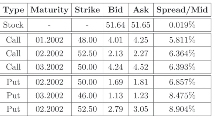
When analyzing option price data one can frequently observe significant bid-ask spreads. For example, Volkswagen stocks were traded with an average relative bid-ask spread of 0.019% at noon on January 03, 2002.1 Table 1 shows the bid-ask spread for call and put
options on Volkswagen at the same point in time. It is obvious that the relative bid-ask spreads of the options are significantly higher than the bid-ask spread of the underlying stock.
Type Maturity Strike Bid Ask Spread/Mid
Stock - - 51.64 51.65 0.019% Call 01.2002 48.00 4.01 4.25 5.811% Call 02.2002 52.50 2.13 2.27 6.364% Call 03.2002 50.00 4.24 4.52 6.393% Put 02.2002 50.00 1.69 1.81 6.857% Put 03.2002 46.00 1.13 1.23 8.475% Put 02.2002 52.50 2.79 3.05 8.904%
Table 1: The relative bid-ask spread of Volkswagen stocks in comparison with relative bid-ask spreads of put and call options on Volkswagen stocks with different strikes and different times to maturity on January 03, 2002.
However, often these bid-ask spreads are neglected in hedging and pricing models, basically for three reasons. First and foremost, no reliable order book data were available until recently that can be used to estimate the implicit transaction costs arising when hedging the option. However, the introduction of automated trading platforms at many exchanges provides new opportunities to develop and implement transaction cost models that make use of the very high granularity and quality of data available in real time in an open electronic order book. Second, existing models that incorporate transaction costs are often not attractive to investors with respect to numerical tractability and computation time. Third, important issues, such as early exercise features of American type options and dividend payments in the underlying, are often ignored in existing transaction cost models.
In our model the bid-ask spread of an option is induced by the costs arising when trading the underlying asset. This relates to the fact that the valuation of options is usually
based on a replication argument which states that an option is priced by the construction of a dynamic trading strategy. This strategy replicates the price process of the option by means of a hedge portfolio at every point in time over the lifetime of the option. By the ’law of one price’ the price of the hedge portfolio and the price of the option has to be the same. In order to use this approach, usually two assumptions are made which refer to the concept of a frictionless market: ”No transaction costs are paid”, and ”The investor can trade assets continuously”. However, when applying standard option pricing models to real-world data these assumptions become problematic since trading in assets always incurs transaction costs and continuous trading is never possible.
The term transaction costs usually consists of two components: explicit an implicit transaction costs. Explicit transaction cost are, for example, fixed fees, taxes, etc. and are incurred during the process of ordering. As mentioned above, in reality security markets are imperfect. As a consequence, it is not possible to buy or sell arbitrary quantities of a security at the theoretical frictionless price. The difference between the frictionless price and the buy or the sell price that can be realized on the market reflects the trading costs and is considered a liquidity premium. This difference is referred to as implicit transaction costs. In the later empirical test of our model we focus on implicit transaction costs, although our model is able to consider explicit transaction costs as well.
Note, that if one replicates an option by a dynamic trading strategy under the as-sumptions of a frictionless market one obtains a unique price for the option. What happens if we allow for transaction costs? When modeling transaction costs in a continuous-time framework the overall costs of rebalancing the hedge portfolio will grow without bounds. In this case transaction costs that arise infinitely often due to rebalancing the hedge port-folio continuously. The infinite amount necessary to replicate the option would imply an infinite option price. Obviously, this is not in line with the concept of no-arbitrage as one can create positions which dominate the option payoff and have a finite price. For exam-ple, for a call option it would be cheaper to perform a simple buy-and-hold strategy in the underlying. If we introduce discrete trading intervals, the overall transaction costs are finite. However, over time this goes along with a growing replication error of the option, and the investor will be exposed to market risk.
One of the first transaction cost models was proposed by Leland (1985). He assumes a continuous price process for the underlying and fixed equidistant intervals between the rebalancing points for the replicating portfolio. By minimizing the variance of the hedging errors, Leland (1985) derives a closed-form solution for the price of a European option
which is similar to the classical Black and Scholes (1973) formula with an adjusted variance term. Instead of minimizing the variance of the hedging errors, Hodges and Neuberger (1989) present an approach in which the chosen strategy maximizes the expected utility of the difference between the realized cash-flow and the desired one at maturity. Merton (1990) develops a replication procedure taking into account proportional transaction costs in a two-period binomial model. This approach was then generalized to the multi-period case by Boyle and Vorst (1992). They derive an adjusted formula similar to the one derived by Leland (1985). This procedure is based on a recursive computation method which allows to price standard options with convex payoff functions.
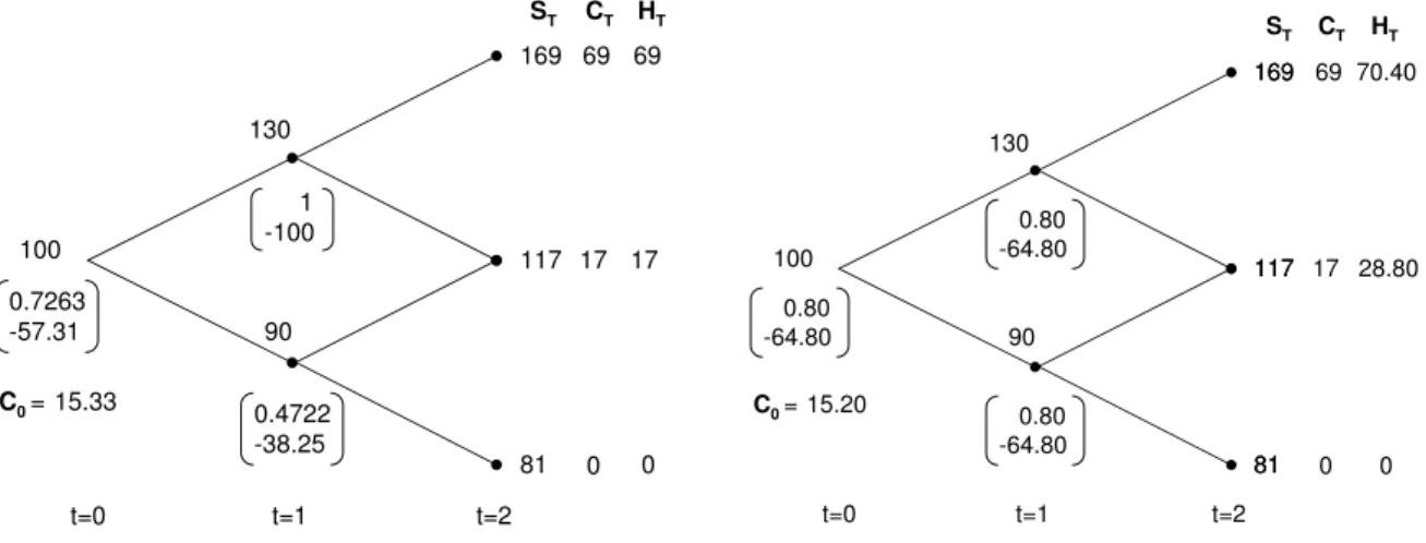
Bensaid, Lense, Pag`es, and Scheinkmann (1992) (BLPS) and Edirisinghe, Naik, and Uppal (1993) (ENU) show that a replicating strategy does not necessarily result in the hedging strategy with the smallest costs. Instead, the hedge portfolio with the smallest costs may be obtained by a strategy which dominates the payoff function of the option in every state. That is, in every state the dominating strategy generates payoffs which are at least as high as the payoffs of the claim, and in some states they are strictly greater. Thus, the authors show that allowing the hedging strategy to dominate the liability instead of matching it perfectly may lower the hedging costs which results in strategies similar to those developed by Constantinides (1986). This type of hedging strategy is referred to as the minimum cost super-hedging strategy. Figure 1 illustrates the idea of super-hedging. The example is taken from Bensaid, Lense, Pag`es, and Scheinkmann (1992).
100 130 90 C T 69 169 117 81 0.7263 -57.31 1 -100 0.4722 -38.25 17 0 H T C 0= 15.33 69 S T 17 0 t=0 t=1 t=2 100 90 130 70.40 169 117 81 0.80 -64.80 28.80 0 HT C0= 15.20 CT 69 169 117 81 17 0 ST 0.80 -64.80 0.80 -64.80 t=0 t=1 t=2
Figure 1: The left tree exhibits an example of a perfect hedging strategy for a call option with strike 100 in a two period binomial tree whereas the left tree displays a super-hedging strategy for the same call option.
H. The two period binomial tree describes the price process of the stock and the hedging strategy is given by the numbers in parentheses. The upper number represents the amount invested in the stock S and the lower number the amount invested in the riskless asset. The perfect hedging strategy leads to C0 = 15.33. The right tree represents a
super-hedging strategy in form of a buy and hold strategy. One can see that in t = 2 in the lowest state the strategy matches the call perfectly whereas in the other two states the strategy generates a surplus. Nevertheless, the resulting price C0 = 15.20 of the call is
smaller than in the case of a perfect hedging strategy. Therefore, it is cheaper to hedge the call by a super-hedging strategy than by a perfect one. This is due to the fact that not rebalancing the hedge portfolio in t = 1 saves more money in form of transaction costs than generating a surplus in t= 2.
The approach discussed in this paper is based on the transaction cost model of ENU. Their approach allows to price the option backward recursively in a binomial tree by means of a dynamic programming procedure which implies several desirable features. In contrast to earlier models the methodology suggested by ENU can be applied to price claims or even a portfolio of claims with different maturities and an overall non-convex payoff structure. Furthermore, by introducing a two-stage dynamic programming optimization algorithm, the size of their model is only quadratic in the trading frequency which is a first step in reducing computation time. The reduction of the state space, introduced by Wehrman (1998) further lowers computation time. In contrast, BLPS treat the whole path of the stock price process as a state variable in their dynamic programming algorithm. In their approach model size grows exponentially in the trading frequency which blows up the computation time especially for options with large times to maturity. In addition, the approach of ENU makes it particularly easy to incorporate an arbitrary transaction costs functional, whereas in most other papers proportional transaction cost were used.
We extend the existing literature in several ways. At many option exchanges, e.g. CBOE, Euronext, ASX, HKE, EUREX, the traded stock options are of American type. This feature is neither considered in the model of ENU nor in the extension of Wehrman (1998). Our model allows to control for early exercise and dividend payments in the underlying. Additionally, we explicitly consider discounting effects by introducing a non-zero interest rate. Our approach is flexible with regard to different settlement schemes. Both, cash settlement as well as physical delivery can easily be implemented in our model. Most importantly, we extend related approaches by introducing a flexible transaction cost functional. Existing models usually assume that arbitrary large amounts of the underlying can be traded at the inside market. In this case the investor has to pay the half spread for
each stock traded. This concept is frequently referred to as proportional transaction costs. However, at the best quotes liquidity is usually limited. Thus, executing large transactions causes a market impact. We model the market impact by a non-linear cost function. Proportional transaction cost and a linear transaction costs are included as special cases. We implement the model using a comprehensive order book data sample for German blue chip stocks which are traded on the automated trading system XETRA. Together with bid-ask spread data for stock options traded at the EUREX, the German electronic trading system for derivatives, this data sample is used to assess the performance of our model. Depending on the hedging strategy applied by the investor the model spread corresponds to roughly three-quarter of the bid-ask spread in a sample consisting of 9,403 option prices.
In order to investigate important properties of our model we analyze the sensitivity of the model spread to variations in the bid-ask spread of the underlying, and to variations in the moneyness, in the volatility, and in the time to maturity of the option.
The remainder of this paper is structured as follows. The general framework is presented in Section 2. The dataset used in the remaining part of the paper is introduced in Section 3. In Section 4 we discuss important properties of the model. Section 5 represents the empirical part of the paper. Here we calibrate our model to order book data for German blue chip stocks and respective stock options. We then calculate the theoretical bid-ask spread for each option in the sample and compare it to the bid-ask spread observed empirically. The paper concludes in Section 6 with a brief summary and a discussion of issues for further research.
2
Theoretical Setup
We consider a multi-period discrete-time binomial model as in Cox, Ross, and Rubinstein (1979). The financial market model is described by a set of finite discrete trading days
t= 0, . . . , T, a stochastic basis{Ω,F,F,P}, and the price processes of the securities traded on the market. T specifies the time horizon of the model which corresponds to the expiry date of the contingent claims considered here. Ω = {ω1. . . ωJ} is a finite state space,
which contains all possible states of the economy. The filtration F ={Ft}Tt=0 models the
arrival of information and is given by a sequence of increasingly finer partitionsFt⊂ Ft+1
(t = 0, . . . , T) of Ω, with F0 = {∅,Ω} and FT = P(Ω). P is a probability measure on Ω
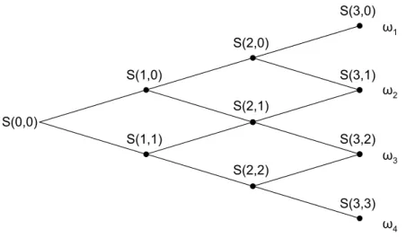
in a event tree as shown in Figure 2 for T = 3, there exists a unique (t−1, i)∈ Ft−1 such
that (t, j) ⊂ (t−1, i). That is, (t−1, i) is the unique predecessor of (t, j). In addition, the element (t, j)∈ Ft has two successors (t+ 1, ju),(t+ 1, jd)∈ Ft+1.
S(0,0) S(1,0) S(1,1) S(2,0) S(2,1) S(2,2) S(3,0) S(3,1) S(3,2) S(3,3) Ȧ1 Ȧ2 Ȧ3 Ȧ4
Figure 2: Recombining binomial tree for T = 3
We assume two traded assets on the market. The first one is a riskless asset B(t), which yields a constant rate of returnrn≥0 over each period of time ∆t= [t, t+ 1]. That
is
B(t+ 1) = (1 +rn)B(t) withB(0) = 1
and the price process of the riskless asset is described by
B(t) = (1 +rn)t witht= 0, . . . , T.
The second traded asset is a risky stock S(t, ω) whose evolution can be represented by a standard binomial model with parameters u, d and r. The parameters un and dn denote
the one period gross return of the stock in case of an up or a down movement. Therefore, the stock is a non-negative and Ft-measurable random variable with price process
S(t+ 1, ju) = unS(t, j) with probability p, S(t+ 1, jd) = dnS(t, j) with probability 1−p,
t = 0, . . . , T −1
where −1≤dn≤1 +rn≤un and un= 1/dn2. The last condition ensures a recombining
binomial tree for the representation of the stock price process, and thus reduces compu-tational complexity. The number of end nodes in an expanded tree grows exponentially
2For the computations in section 4 and 5 we use (1 +r
n) =er∆twhere r is the continuous time spot rate. We set ∆t=T /nand divide [0, T] inton equal subintervals. Furthermore we useun =eσ
√
∆tand
dn=e−σ
√
inT, whereas the recombining tree only grows quadratic in T. For recursive algorithms in an event tree only the use of a recombining tree results in acceptable computation time for large T.
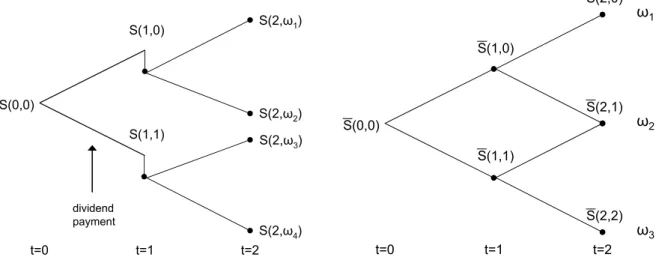
Our setup allows to consider the payment of one known Dollar dividend within the lifetime of the claim. Generally, the existence of such a dividend destroys the recombining property of the binomial tree as it is exemplarily displayed in the left tree of Figure 3. However, to maintain the features of a recombining tree we adopt an algorithm which can be traced back to Roll (1977).
S(0,0) S(1,0) S(1,1) S(2,Ȧ2) t=0 t=1 t=2 dividend payment S(2,Ȧ1) S(2,Ȧ3) S(2,Ȧ4) Ȧ1 S(0,0) S(1,0) S(1,1) S(2,0) S(2,1) S(2,2) t=0 t=1 t=2 Ȧ2 Ȧ3
Figure 3: The left tree shows a non-recombining binomial tree due to a payment of one known Dollar dividend. The right tree exhibits the fixed recombining tree which approx-imates the the true stock price S process by S.
Here the stock price S is split up into two components. One part S∗ is uncertain. The other one D is certain representing the present value of all future dividends during the lifetime of the claim. Without loss of generality we assume that the point in time when the dividend is paid, denoted byτ, lays within a time period rather than on a rebalancing point. The value of the uncertain component S∗ at timen∆t is given by
S∗ =S forn∆t > τ and by
S∗ =S−De−r(τ−n∆t) forn∆t≤τ.
Starting in t = 0 the present value of the future dividend is added at each node to the uncertain stock price component S∗. Thus, we can model the true stock price process of
S in a recombining tree by the approximating stock price process S (see the right tree in Figure 3). That is, at time n∆t the approximating stock price S at each node (n∆t, j) is given by
S∗(0,0)u(n−j)dj +De−r(τ−n∆t), j = 0, . . . , n
as long as n∆t < τ, and
S∗(0,0)u(n−j)dj, j = 0, . . . , n
as soon asn∆t ≥τ. The value of the uncertain component S∗(0,0) at time t= 0 can be calculated as
S∗(0,0) = S(0,0)−De−rτ.
A contingent claim on the market is defined as a two dimensional random variable
X = (gT, hT), where gT and hT represent the number of shares and the amount of cash
transferred from the writer of the claim to its holder at the time of expiration T (or conversely, depending on the sign of gT and hT). A long position in a European call
option with strike priceK and physical delivery is therefore described by
CTe =¡I{ST>K},−KI{ST>K}
¢ .
That is, at maturity an in-the-money call option is represented by a portfolio consisting of one stock and a short position of amount K in the riskless asset. Correspondingly, a long position in an American call option with strike priceK and physical delivery is described by the claim Ca t=τ∗ = ¡ I{t=τ∗},−KI{t=τ∗} ¢ ,
where τ∗ denotes the exercise time of the option which is assumed to be the optimal stopping time for the price process of the American option.
We refer to φt = (α(t, j), β(t, j)) with t = 0, . . . , T and j = 0, . . . , t as a trading
strategy whereα(t, j) denotes the number of stocks andβ(t, j) the dollar amount invested in the risk-free asset at time t and in node j. Trading the stock incurs transaction costs
θ(∆α(t, j)), where ∆α(t, j) = (α(t, j)−α(t−1, i)) is the number of shares sold or bought at time t. In our case θ(∆α(t, j)) is a cost functional which is related to the number of traded shares defined in the following way
θ(∆α(t, j)) =a+b|∆α(t, j)|c. (1)
Thus, in general, buyingone share costsS(1 +θ), and the amount you receive for selling
one shares is S(1−θ). Consequently, buying ∆α shares results in costs amounting to ∆α·S(1+θ(∆α)), and the amount you receive for selling ∆αshares is ∆α·S(1−θ(∆α)).
In the special case where a > 0 and b = 0 (with carbitrarily chosen), we have the case of proportional transaction costs. Hence, in our case the parametera represents half of the best bid-ask spread (inside market), which is the minimum amount of transaction cost you have to pay in order to trade the stock. A large trade which consumes more liquidity as provided at the best quote has a price impact. This price impact is modeled by the parameters b and c. For a > 0, b > 0 and c ≡ 1 we have a linear price impact function. For a >0,b > 0 andc >0 we have a non-linear price impact function.
2.1
The Model
Our objective is to find the self-financing hedging strategy of the claim X which mini-mizes the financing cost in t = 0, subject to self-financing constraints and the terminal constraints. Thus, the investor´s problem, denoted byP1, is formally stated as follows:
X0 = min {α,β} £ α(0,0)S(0,0) +β(0,0) + [|α(0,0)|θ(α(0,0))S(0,0)]I{tc0>0} ¤ , (2)
subject to the self-financing constraints,
α(t−1, i)S(t, j) +β(t−1, i) ≥ α(t, j)S(t, j) +β(t, j)
+|α(t, j)−α(t−1, i)|θ(t, j)S(t, j), (3)
∀j ∈ Ft, j ⊂i, i∈ Ft−1, t = 1, . . . , T −1,
and subject to the terminal constraints,
α(T −1, i)S(T, j) +β(T −1, i) ≥ X(T, j) +|α(T, j)−α(T −1, i)|θ(T, j)S(T, j)I{tcT>0} ⇔ α(T −1, i)S(T, j) +β(T −1, i) ≥ α(T, j)S(T, j) +β(T, j) +|α(T, j)−α(T −1, i)|θ(T, j)S(T, j)I{tcT>0},(4) ∀j ∈ FT, j ⊂i, i∈ FT−1, with α(T, j) =g(T, j) and β(T, j)≥h(T, j).
Notice, that the constraints (3) and (4) are stated as inequalities, which is due to the fact, that in the presence of transaction costs it may sometimes be optimal to super-hedge
the claim rather than replicating it exactly. The self-financing constraints in (3) require that the value of the old portfolio composition is high enough to finance the revision of the portfolio, even after taking into account the transaction costs. It should be noted that the indicator function I{tc0>0} is equal to 1 if transaction costs are incurred when
setting up the hedging portfolio which means, there are no holdings in the assets int= 0. Analogously, I{tcT>0} in the terminal constraints (4) is equal to 1 if there are transaction
costs in T, that is, the claim is settled by delivery. Given the shape of (3) and (4), P1 is a non-linear optimization problem solved by a recursive algorithm presented in the next paragraph.
2.2
Recursive Algorithm
We now formulate a dynamic programming procedure, which solves the cost minimization problem P1, on a three dimensional state space spanned by the portfolio weights α, β, and the stock price process S. By modeling the stock price process in a binomial tree the dimension of the state space reduces to two. If we also assume that it is possible to invest an arbitrary amount into the riskless asset, then we are further able to reduce the dimensionality to one. That is, in order to solve our problem by applying a dynamic programming procedure, we only need to discretize the state space of the portfolio weights for the stock. This results in feasible computation times.
The optimization problem is solved in two steps. At the first stage, the minimal value of the replication portfolio is computed for every possible starting weight of the stock in our discretized state space. That is, for each position in the stock at t= 0 we are looking for a self-financing trading strategy that super-hedges the claim in every point in time. This can be done by a recursive approach. The approach yields, for a given starting position in the stock, the amount one has to invest in the riskless asset such that one can always continue the replication procedure without incurring a loss until maturity. At the second stage, we simply search for the cost minimizing portfolio composition in t= 0.
The state space of the portfolio weights of the stock depends on the type of the claim to be replicated. For example, if we want to replicate a long position in a call, the weights of the stock are elements of the interval [0,1]. Therefore, we can describe the state space of the portfolio weights of the stock by an equidistant discretization of the interval [0,1], that is
Note, that an investor normally does not buy a single option but a contract consisting of
s∈Noptions. The quantity δα =s−1 can be interpreted as a lot size and reflects the fact
that investors are usually constrained to trade a minimum number of options.
2.2.1 Start of the Recursion
The amount to be invested in the riskless asset at each point in time is given by the value function V which in turn depends on the current stock price S(t, j) as well as on the current holdings in stocks α(t, j).
At time t =T −1 the value function is determined by the terminal constraints in the end nodes and is given by
V(αT−1, S(T −1, j)) :=R−1max h βαupT−1, βαdownT−1 i (5) ∀j = 0, . . . , T −1 and ∀αT−1 ∈A withR =er∆t.
The value of V at timeT −1 corresponds to the amount invested in the riskless asset at the risk-free interest rate r which ensures that the payoff profile of the claim X is met, no matter if an up move (node (T, j)) or a down move (node (T, j+ 1)) in the stock price occurs. The variable βup
αT−1 denotes the amount invested in the riskless asset sufficient to
guarantee a super replication in the case of an up move. The variable βdown
αT−1 denotes the
respective quantity for a down move. The variables are defined as follows:
βup αT−1 = βαT−1(αT =gT, S(T, j)) := X(T, j)−αT−1S(T, j) + [|α(T, j)−αT−1|θ(T, j)S(T, j)]I{tcT>0} (6) βαdownT−1 = βαT−1(αT =gT, S(T, j+ 1)) := X(T, j+ 1)−αT−1S(T, j+ 1) + [|α(T, j+ 1)−αT−1|θ(T, j+ 1)S(T, j+ 1)]I{tcT>0} (7) ∀j = 0, . . . , T −1 ∀αT−1 ∈A.
According to Equation 5 the value function corresponds to the discounted maximum of
βup
αT−1 and β
down
2.2.2 Recursion Step
Now, for every recursion stept+1 totwe have to compute the value functionV as follows
V(αt, S(t, j)) :=R−1max £ βup αt, β down αt ¤ (8) ∀t = 0, . . . , T −2 and ∀ j = 0, . . . , t.
For an up move and a down move of the stock, respectively,
βup αt := minα t+1∈A [βαt(αt+1, S(t+ 1, j))] (9) and βdown αt := minα t+1∈A [βαt(αt+1, S(t+ 1, j+ 1))] (10)
denote the quantities invested in the riskless asset that ensure the continuation of the self-financing super-hedging strategy for a given αt. The early exercise features of American
type options need to be considered in the self-financing constraint. Let Xh denote the
value of the claim if it is held over the next period of time, and let Xex denote the value
of the claim if it is exercised immediately. Then, βαt(αt+1, S(t+ 1, j)) is given by
βαt(αt+1, S(t+ 1, j)) := ( βh αt(αt+1, S(t+ 1, j)) : X h(t+ 1, j)≥Xex(t+ 1, j) βex αt(αt+1, S(t+ 1, j)) : otherwise , (11) where βh αt(αt+1, S(t+ 1, j)) := V(αt+1, S(t+ 1, j)) + (α(t+ 1, j)−αt)S(t+ 1, j) +|α(t+ 1, j)−αt|θ(t+ 1, j)S(t+ 1, j) (12) and βαext(αt+1, S(t+ 1, j)) := Xh(t+ 1, j)−αtS(t+ 1, j+ 1) +[|α(t+ 1, j)−αt|θ(t+ 1, j)S(t+ 1, j+ 1)]I{tcT>0}, (13) ∀t= 0, . . . , T −2, ∀j = 0, . . . , t, ∀αt ∈A.
If the value of exercising the option is greater than the value of holding it for one more period, the investor will exercise the option. This has to be taken into account for the hedging procedure.
2.2.3 Determining the value of the claim
At the end of the recursion algorithm in t = 0, a search over all portfolio weights of the set A is required to identify the portfolio compliance with the least initialisation costs. This can be formulated as
X0 = min α0∈A £ α0S(0,0) +β(0,0) + [|α0|θ(α0)S(0,0)]I{tc0>0} ¤ , (14) where β(0,0) = V(α0, S(0,0)).
Considering transaction costs for setting up the initial hedge portfolio int= 0 is equivalent toI{tc0>0} = 1.
3
Dataset
In order to explore the properties of our model and to test its overall performance we analyze the spreads of options on stocks included in the German blue chip index DAX over the first quarter of 2002 with a total of 61 trading days. The DAX index contains the largest German companies in terms of order book volume and market capitalization. A summary of the index composition is given in the Appendix. We use a stock and an option sample consisting of time-stamped order book sequences and bid-ask spread data from XETRA and EUREX, the automated electronic stock and option exchanges in Germany. Both trading platforms offer an open order book to investors that can be used to assess the current market liquidity. The order book data for the stocks traded in XETRA allow us to estimate the implicit transaction costs that an investor has to bear when hedging an option dynamically. The bid-ask spread data of stock options is used to compute the implicit volatility of the analyzed options, and serves as a benchmark for our model prices are compared with.
Trading hours for stocks and options traded in XETRA and at the EUREX respec-tively in 2002 were from 9:00 a.m. to 8:00 p.m. However, we assume that our investor adjusts the hedge portfolio only on a daily basis at 1:00 p.m. in a single transaction.
We begin our sample selection with all DAX companies except for Preussag (now TUI) due to a lack of option data for this company. We exclude option contracts from our sample with less than seven days to maturity to avoid potential liquidity effects or pricing biases as found, for example, in Kalay and Subrahmanyam (1984) and Schlag
(1996). Furthermore, we eliminate illiquid options, i.e., options whose bid-ask spread has not been updated within the last 60 minutes prior to data collection. Furthermore, we concentrate our analysis on options with less than 74 days to maturity. Thus, we end up with 9,403 options (4,695 call and 4708 put options) that are used to calibrate and test the model. For 894 of the 4,695 call options and for 871 of the 4708 put options we observed a dividend payment in the underlying during their lifetime. From the 29 underlying stocks 25 paid a dividend during our sample period. The average dividend yield was 1.98%.
4
Properties of the Model
In order to investigate the properties of our model we want to focus just on one benchmark case. Therefore, we choose one call option on Volkswagen from our data sample whose characteristics are given in Table 2.
Underlying Volkswagen Trading day January 03, 2002 Maturity (in days) 31
Strike 52.50
Midprice of the Underlying 51.65 Implied volatility 0.35 Best bid price of the option 2.13 Best ask price of the option 2.27 Mid price of the option 2.20 Riskless interest rate (in %) 3.32
Table 2: Characteristics of the benchmark call option on Volkswagen used to investigate important properties of the model.
In this section we want to address basically three issues: First, we look at the overall transaction costs that have to be paid when setting up the hedging portfolio initially, when adjusting the hedge portfolio throughout the lifetime of the option, and at the expiry of the option. Second, we analyze the sensitivity of the bid ask spread to variations in the bid-ask spread of the underlying, and to variations in the moneyness, in the volatility, and in the time to maturity of the option. Third, we examine the variation of the bid-ask spread if different transaction cost functions are taken into consideration.
With respect to the first issue we distinguish between three cost components: the initial transaction costs (tc0) needed to the set up of the hedge position in t = 0, the
transactions costs (tcr) paid for rebalancing the hedge portfolio over the life time of the
option, and the transaction costs (tcT) paid at maturity. The cost componenttcris relevant
for every investor who wants to hedge the option dynamically. However, the other two components might not be relevant for institutional investor holding a large position in the underlying anyway. For the analysis of the first two issues we assume that the investor can always trade at the best bid or the best ask price. For the third issue we assume that the investor hedges a large portfolio of options such that the rebalancing of the hedge portfolio causes a market impact. Given this assumption the definition of the price impact function becomes relevant.
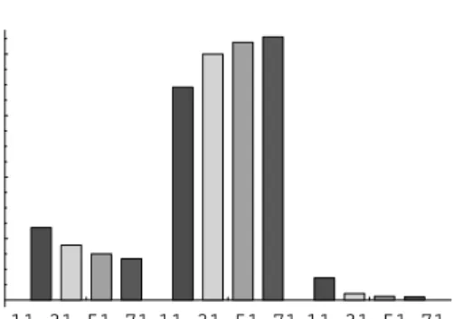
For our benchmark case we obtain the following results:tc0 = 17.87%,tcr = 79.99%, tcT = 2.14%. Thus, the vast part of transaction costs has to be paid when adjusting the
hedge portfolio throughout the remaining lifetime of the option. As one can see in Figure 4 this ratios will change if the time to maturity is varied. If the time to maturity is reduced
tc0 and tcT become more relevant.
11 31 51 71 tc0 11 31 51 71 tcr 11 31 51 71 tcT T in days, cost components 20 40 60 80 In % of overall transaction costs
Figure 4: Composition of overall transaction costs for different maturities (11, 31, 51, and 71 days).
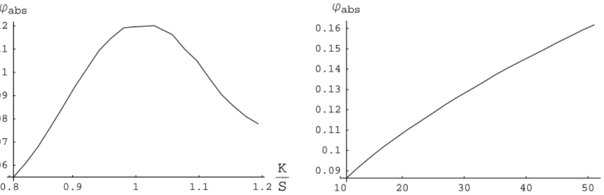
Next, we perform a sensitivity analysis for our benchmark scenario and vary the pa-rameters: moneyness, maturity, spread of the underlying, and volatility of the underlying. When varying the strike price of the benchmark call option we observe the highest absolute bid-ask spreads for options approximately at-the-money. This seems intuitively reasonable as those options exhibit the highest gamma. Thus, for those options the investor
has to rebalance the hedge portfolio more often compared to options which are deeply in or out of the money. Rebalancing the hedge portfolio causes transaction costs, and thus increases the bid-ask spread in the corresponding option.
0.8 0.9 1 1.1 1.2 K S 0.06 0.07 0.08 0.09 0.1 0.11 0.12 jabs 10 20 30 40 50 T 0.09 0.1 0.11 0.12 0.13 0.14 0.15 0.16 jabs
Figure 5: Sensitivity of the absolute bid-ask spread ϕabs of the option w.r.t. moneyness
(left) and time to maturity T (right) of the option
When varying the time to maturity of the option we can observe increasing bid-ask spreads. A longer time horizon implies more adjustments of the hedge portfolio and thus increases the spread of the option.
A similar effect might help to explain the relationship between the half spread in the underlying and the bid-ask spread in the underlying. Increasing the first rises the transaction costs an investor has to bear when rebalancing a hedge portfolio almost pro-portionally. However, if the spread in the underlying increases significantly super-hedging may be optimal. Thus, one should not expect a stable linear relationship between higher values of the half spread in the underlying and the bid-ask spread of the option.
0.002 0.004 0.006 0.008 0.01 a 0.5 1 1.5 2 2.5 3 3.5 jabs
Figure 6: Sensitivity of the absolute bid-ask spreadϕabsof the option w.r.t. the half spread
If we vary the volatility of the underlying we only observe minor variations in the bid-ask spread. For example, a change in volatility from 20% to 40% increases the spread of our benchmark option by less than 1 cent.
In order to compare different specifications of the transaction cost function 1 we first calibrate all three choices (proportional transaction costs, linear, and non-linear transac-tion cost functransac-tional) to the order book data for Volkswagen and obtain the following results:
proportional transaction costs : θ(∆α) = 0.000381073
linear market impact : θ(∆α) = 0.000014 + 0.00107|∆α|
non-linear market impact : θ(∆α) = 0.000627 + 0.000508|∆α|1.3989.
Note, that θ(∆α) is a percentage quantity. Therefore, buying one Volkswagen share at the inside market results in transaction costs of 0.000381073·51.65 = 0.01968 Euros.
-5 -4 -3 -2 -1 0 1 2 3 4 5 6 DΑ 0.02 0.06 0.1 0.14 0.18 0.22 0.26 0.3 0.34 0.38 0.42 tca -5 -4 -3 -2 -1 0 1 2 3 4 5 6 DΑ 0.02 0.06 0.1 0.14 0.18 0.22 0.26 0.3 0.34 0.38 0.42 tca
Figure 7: The estimated transaction costs (solid line), linear (left) and non-linear (right), is plotted versus the observed orderbook data (dashed line) and the estimated half spread (dotted-dashed line)
The estimated transaction costs are shown in Figure 7. The horizontal axis measures the rebalancing volume ∆α given in tens of thousands of shares. The vertical axis shows the respective amount of transaction costs that has to be paid when trading ∆α shares. The dashed line in the graph represents the empirical average calculated over 61 trading days for Volkswagen stocks, and the solid line shows the calibrated cost functions. The dotted dashed line indicates the case of proportional transaction costs.
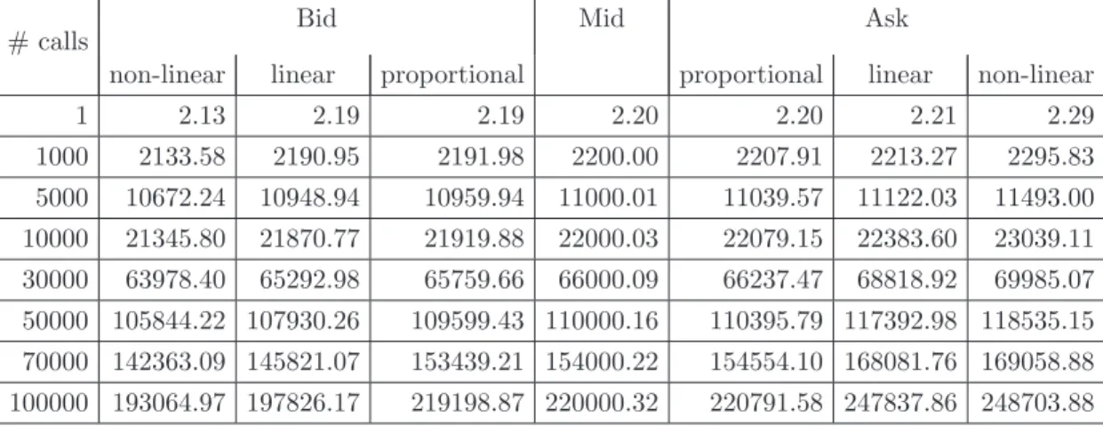
Next, we are able to calculate the resulting bid-ask spreads for the different amounts of options to be hedged. Table 3 provides the results. As expected applying the non-linear
# calls Bid Mid Ask
non-linear linear proportional proportional linear non-linear
1 2.13 2.19 2.19 2.20 2.20 2.21 2.29 1000 2133.58 2190.95 2191.98 2200.00 2207.91 2213.27 2295.83 5000 10672.24 10948.94 10959.94 11000.01 11039.57 11122.03 11493.00 10000 21345.80 21870.77 21919.88 22000.03 22079.15 22383.60 23039.11 30000 63978.40 65292.98 65759.66 66000.09 66237.47 68818.92 69985.07 50000 105844.22 107930.26 109599.43 110000.16 110395.79 117392.98 118535.15 70000 142363.09 145821.07 153439.21 154000.22 154554.10 168081.76 169058.88 100000 193064.97 197826.17 219198.87 220000.32 220791.58 247837.86 248703.88
Table 3: Bid and ask prices for different quantities of options traded and for different order book impact functions
cost function yields the widest spreads. However, the differences to the case of a linear-cost function are only moderate. Modeling only proportional transaction linear-costs results in constant bid-ask spreads. No matter, how many options are hedged, the investor always pays the same amount of transaction costs for each stock traded.
5
Empirical Analysis of Stock Option Spreads
In order to test our model we calculate the bid-ask spreads for all 9,403 options using our transaction cost model. We consider two different scenarios. In the first case, we incorporate all three transaction cost components, tc0, tcr, and tcT. In the second case,
we leave out the tc0 part which relates to a situation where a large investor has already
large holdings in the underlying and therefore does not have to bear any cost while setting up the hedge portfolio initially.
To compare our theoretical results with the empirical data we compute the ratio between the empirical bid-ask spread ϕe and the model bid-ask spread ϕm. The ratio,
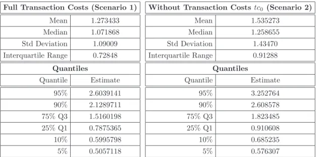
thereafter referred to as spread ratio, is plotted in Figure 8, and summary statistics are given in Table 4. As one can observe in the histograms for both cases a large part of the probability mass is distributed closely around 1. A ratio of exactly one indicates that the model spread coincides with the empirical spread. A value greater than one shows up if the model underestimates the empirical spread of the option.
The quantiles given in table 4 provide strong evidence that our model is able to explain a significant part of the bid-ask spread observed empirically. On average we found
0.5 1 1.5 2 2.5 3 3.5 4je jm 0.1 0.2 0.3 0.4 0.5 0.6 0.7 0.8 0.9 1 fi 0.5 1 1.5 2 2.5 3 3.5 4je jm 0.1 0.2 0.3 0.4 0.5 0.6 0.7 0.8 fi
Figure 8: Histogram of the spread ratio for scenario 1 (all transaction cost incorporated) (left) and scenario 2 (without transaction cost in t = 0) (right).
Full Transaction Costs (Scenario 1)
Mean 1.273433 Median 1.071868 Std Deviation 1.09009 Interquartile Range 0.72848 Quantiles Quantile Estimate 95% 2.6039141 90% 2.1289711 75% Q3 1.5160198 25% Q1 0.7875365 10% 0.5995798 5% 0.5057118
Without Transaction Costs tc0 (Scenario 2)
Mean 1.535273 Median 1.258655 Std Deviation 1.43470 Interquartile Range 0.91288 Quantiles Quantile Estimate 95% 3.252764 90% 2.608578 75% Q3 1.823485 25% Q1 0.910608 10% 0.685235 5% 0.576307
Table 4: Summery statistics for the spread ratio in scenario 1 (left) and scenario 2 (right)
a spread ratio of 1.27 in scenario 1 and 1.54 in scenario 2. Thus, the assumptions made for scenario 1 are more suitable to reproduce the bid-ask spreads in the option market than the assumptions underlying scenario 2. In scenario 1 the model spread corresponds on average to 78% of the empirical bid-ask spread in our sample consisting of 9,403 option prices. In more than 50 percent of all observations the coefficient lies between 0.78 and 1.51, and the median is given by 1.03. Overall, the model seems very well specified.
Figure 9 shows histograms of spread ratios calculated under the assumption of sce-nario 1. The left graph of Figure 9 displays the spread ratios for options on non-dividend paying stocks. The right graph represents these ratios for options on dividend paying stocks. In both cases we use the assumptions made for scenario 1. For non-dividend
pay-0.5 1 1.5 2 2.5 3 3.5 4je jm 0.1 0.2 0.3 0.4 0.5 0.6 0.7 0.8 0.9 fi 0.5 1 1.5 2 2.5 3 3.5 4je jm 0.1 0.2 0.3 0.4 0.5 0.6 0.7 0.8 0.9 1 1.1 1.2 1.3 1.4 fi
Figure 9: Histograms of the spread ratio for options on non-dividend paying stocks (left) and for options on dividend paying stocks (right) under scenario 1.
ing stocks the results are similar to those represented above for the overall sample. For dividend paying stocks the model seems to overestimate the empirical bid-ask spread slightly. When dividends are paid it may be optimal to exercise call options early im-mediately before the stocks goes ex-dividend. In those situations the short party has to deliver the stock physically which causes high transaction cost at an early stage and that translates into high model spreads.
6
Conclusion
In this paper we extend the transaction cost model proposed by ENU and Wehrmann in order to incorporate the early exercise feature of American options, physical delivery of the underlying at expiry of the option, and dividend payments in the underlying. These issues are relevant when analyzing empirical option price data.
To explore important properties of our model and to analyze its pricing performance we use a representative data sample collected in 2002 for German blue chip stocks and the respective options traded at the EUREX.
In our model the bid-ask spread is higher for at-the-money options than for options which are deeply in or out of the money. It increases with respect to the time to maturity and the half spread of the underlying. Taking the mean (median), our model spread corresponds on average to 78% (93%) of the empirical bid-ask spread in a sample consisting of 9,403 option prices.
spread and the volatility of the underlying. In reality these variables vary through time. Thus, further research could focus on the introduction of more sources of risk, e.g., liquidity and/or volatility risk. Furthermore, it might be interesting to investigate the impact of transaction costs on the pricing of exotic options and to analyze whether the early exercise decision for American options is influenced by the presence of transaction costs.
7
Appendix
Company name Weight in Turnover in XETRA Avg. trade size Avg.
bid-ask-DAX (in %) (Millions of e, (Thousands ofe, spread, (e, Jan. 7, 2002) Jan. 7, 2002) Jan. 7, 2002)
Adidas-Salomon 0.50 27.3 41.6 0.22 Allianz 9.50 252.3 107.1 0.26 BASF 3.58 152.4 71.4 0.04 Bayer 3.75 130.1 62.1 0.05 BMW 3.66 87.9 63.8 0.07 Commerzbank 1.35 38.4 35.3 0.04 DaimlerChrysler 6.79 326.9 85.0 0.04 Degussa 0.83 16.1 28.2 0.13 Deutsche Bank 6.81 321.9 97.2 0.05 Deutsche Post 1.23 45.1 37.7 0.05 Deutsche Telekom 11.15 378.0 85.8 0.02 E.ON 5.80 165.4 74.4 0.06 Epcos 0.53 25.9 28.0 0.13
Fresenius Med. Care 0.81 21.0 39.0 0.18
Henkel 1.26 21.3 43.9 0.16 Hypovereinsbank 2.50 75.9 44.2 0.06 Infineon 2.46 167.2 48.3 0.05 Linde 0.76 18.8 34.6 0.11 Lufthansa 0.87 122.8 52.2 0.03 MAN 0.51 16.2 29.3 0.09 Metro 1.81 46.2 32.3 0.09 MLP 0.84 26.6 74.7 0.23 M¨unchener R¨uck 7.22 204.1 101.4 0.27 Preussag 0.79 27.4 29.2 0.09 RWE 3.17 63.8 47.4 0.07 SAP 6.55 346.8 94.4 0.18 Schering 1.54 75.0 49.9 0.08 Siemens 9.18 576.7 97.3 0.06 ThyssenKrupp 1.20 41.4 34.2 0.04 Volkswagen 3.06 108.3 54.1 0.06
Table 5: The table contains the constituents of the DAX index, the percentages of the individual shares in the index, the turnover of the respective shares in XETRA on January 7, 2002, the average trade size in thousands of e, and the average bid-ask-spread on January 7, 2002. Source: B¨orsenzeitung, January 8, 2002 and own calculations.
References
Bensaid, B., J.-P. Lense, H. Pag`es, and J. Scheinkmann, 1992, Derivative Asset Pricing with Transaction Costs, Mathematical Finance 2, 63–86.
Black, F., and M. Scholes, 1973, The Pricing of Options and Corporate Liabilities,Journal of Political Economy 81, 637–654.
Boyle, P. P., and T. Vorst, 1992, Option Replication in Discrete Time with Transaction Costs,Journal of Finance 47, 271–293.
Constantinides, G. M., 1986, Capital Market Equelibrium with Transaction Costs,Journal of Political Economy 94, 842–862.
Cox, J.C., S.A. Ross, and M. Rubinstein, 1979, Option pricing: A Simplified Approach,
Journal of Financial Economics 7, 229–263.
Edirisinghe, C., V. Naik, and R. Uppal, 1993, Optimal Replication of Options with Trans-action Costs and Trading, The Journal of Financial and Quantitative Analysis 28, 117–138.
Hodges, S.D., and A. Neuberger, 1989, Optimal Replication of Contigent Claims under Transaction Costs, Review of Future Markets 8, 222–239.
Kalay, A., and M. Subrahmanyam, 1984, The Ex-Dividend Day Behavior of Option Prices,
Journal of Business 57, 113–128.
Leland, H.E., 1985, Option Pricing and Replication with Transactions Costs, Journal of Finance 40, 1283–1301.
Merton, R. C., 1990, Continuous-Time Finance. (Blackwell Publishers Ltd).
Roll, R., 1977, An Analytical Valuation Formula for Unprotected American Call Options on Stock with Known Dividends,Journal of Financial Economics 5, 251–258.
Schlag, C., 1996, Expiration Day Effects of Stock Index Derivatives in Germany,European Financial Management 2, 69–95.
Wehrman, Dirk C., 1998, Strategien zur Absicherung ungewisser Verpflichtungen mit Transaktionskosten im Binomialmodell vol. 4 ofKarlsruher Reihe. (VVW Karlsruhe).