The Hidden Cost of Priority Dispatch for Wind Power

The Hidden Cost of Priority Dispatch for Wind Power

Department of Industrial Engineering and Operations Research, Tsinghua-Berkeley Shenzhen Institute,

University of California Berkeley [email protected]

Shmuel Oren

Department of Industrial Engineering and Operations Research, Tsinghua-Berkeley Shenzhen Institute,

University of California Berkeley [email protected]

Abstract

Rrenewable generation, such as wind power, is com-monly considered a must-take resource in power sys-tems. In this work we show that, given the technical ca-pabilities of current wind turbines, this approach could lead to major economic inefficiency as wind integration levels in power systems increase. We initially provide intuition for cases in which the optimal operating point involves shedding renewable generation, even though no cost is associated with it in the optimization objective, illustrated in small power systems. We then explore the expected benefit from dispatching wind resources at a lower level than their available output in a Stochastic Unit Commitment (SUC) framework. The modeling and evaluation approach adopted are described. A decom-position technique based on recent literature that uti-lizes global cuts and Lagrangian penalties to achieve convergence is used to solve the resulting large scale mixed integer optimization problem, in a high perfor-mance computing environment. A reduced California system is examined as a test case.

1.

Introduction

The worldwide drive towards a cleaner and sustain-able electricity generation mix has lead to increased re-newable integration goals for the coming years. Cali-fornia, for example, is on track for achieving its 2020 goal of33% of energy needs satisfied by renewable re-sources and now aims for50% by 2030 [1]. Renew-able resources have been traditionally treated - and are still treated by many system operators - as must-take resources (negative load), i.e. they are fully integrated in the electricity network regardless of their level or variability. Renewable curtailments only occur in cases where operational feasibility is at risk. The increased renewable integration, however, gradually brings about new operating conditions, such as steeper power ramps, overgeneration and decreased frequency response capa-bilities. Conventional generation by itself is unable or

extremely costly to deal with these new conditions and a paradigm shift is necessary, in which renewable gen-eration is called upon to contribute to ancillary services and grid flexibility by systematically dispatching at lev-els defined by operational and cost considerations. The need for such policies is already becoming apparent in regions with increased renewable integration; the Cali-fornia Independent System Operator (CAISO) curtailed about 1% of the total potential renewable generation during the first quarter of2017, with solar curtailment reaching up to30% at specific times, while it has already adopted market based curtailment mechanisms [2]. In Europe, on the other hand, directive 2009/28/EC is cur-rently in force and stipulates by law that “Member States shall ensure that when dispatching electricity generating installations, transmission system operators shall give priority to generating installations using renewable en-ergy sources in so far as the secure operation of the na-tional electricity system permits and based on transpar-ent and non-discriminatory criteria” [3].

We focus on mobilizing the flexibility of wind dis-patch. Current wind generators and power plants have advanced controls that allow them to operate practi-cally at any point below their (maximum) available out-put [4, 5]. However, their available outout-put itself depends on the weather conditions, i.e. the availability of wind. Consequently, they are considered semi-dispatchable (in contrast to conventional resources for which complete control over the output point is possible). These techni-cal capabilities, however, enable us to consider the opti-mization of the wind generation setpoint, instead of inte-grating all of the available wind generation into the sys-tem. The benefits from curtailing wind production have been examined from various perspectives. In [6] and [7], NREL provides a series of cases of wind curtailment in systems in the US or abroad. In [8] and [9] CAISO uses the software PLEXOS to simulate a rolling unit commit-ment problem in the presence of wind curtailcommit-ment for high wind penetration. In [10] it is shown that allowing for renewable curtailment enables significant reduction of the required system storage size, in [11] the benefits

Proceedings of the 52nd Hawaii International Conference on System Sciences | 2019

are motivated mainly through solving a Security Con-strained Optimal Power Flow (SCOPF) problem, in [12] through a market coupling and a nodal pricing model of part of the European system, in [13, 14] through a Secu-rity Constraint Unit Commitment (SCUC) Problem and in [15] a dynamic interaction of wind curtailment with storage is examined when the ramping rates of power plants are considered. An overview of the motivation be-hind wind curtailment is given in [16], whereas in [17] wind curtailment is employed for active network man-agement. A flexible wind dispatch margin for the joint energy and reserves market and offline policies to obtain it are examined in [18] and [19].

We decided to motivate flexible wind dispatch in the context of the Stochastic Unit Commitment (SUC) problem instead. The Unit Commitment problem is a widely studied mixed integer program [20–22] that de-termines the set of generators, among all the available ones, that will be committed to satisfy the load dur-ing the followdur-ing day. The two stage Stochastic Unit Commitment problem (SUC) formulates the same deci-sion in the presence of uncertainty (renewable genera-tion, faults, load), captured by a finite set of possible re-alizations (scenarios) [23–27]. While wind curtailment is a usual assumption when formulating the SUC prob-lem, in this work we explicitly focus on calculating the expected benefit from optimizing the wind output set-point versus an approach that treats wind as a priority resource. A similar approach appears in [28], where coordination with storage is considered to illustrate the benefits from dispatchable wind. The size of the op-timization problem scales linearly with the number of scenarios and for that purpose a large amount of research has been devoted to decomposition techniques to itera-tively approximate the solution of the problem. Among these, in [29], the Progressive Hedging (PH) algorithm is adapted to successfully solve the SUC problem. In [30] a cutting plane algorithmic approach is used. In [31] a parallel implementation of Lagrangian relaxation in a high performance computing environment is employed. In [32] an asynchronous parallelized algorithm based on stochastic subgradient is utilized to efficiently solve the problem.

In this work, we provide a complete framework to understand and evaluate the expected benefit from flex-ible wind dispatch in a SUC setting, while also intro-ducing innovations in the implementation of the various components of the model. To begin with, since wind generation is not associated with any fuel costs in the objective, it is not self evident why we could be better off curtailing it and using costly conventional genera-tion in its place. For this reason, we present small mo-tivating examples to offer intuition regarding the most

common setups where such benefit may occur: opera-tion during oversupply, ramping requirements, technical minima of generators and congestion. We then proceed to describe the complete evaluation framework, by intro-ducing its basic components: the Uncertainty and Opti-mization Modules.

The Uncertainty Module is responsible for generat-ing sample scenarios that capture the underlygenerat-ing uncer-tainty for renewables and system faults. It is based on existing wind speed modeling techniques, which we ex-tend by using a non parametric modeling methodology for the aggregate power curve, i.e. the mapping of wind speed to wind generation, utlizing local polynomial re-gression [33]. The Optimization module, on the other hand, is responsible for solving the SUC problem given a set of scenarios. It specializes an algorithm presented in [34] for general two stage stochastic programs with binary first stage variables. The intuition behind the al-gorithm is that, if the different scenarios of a stochas-tic program are similar, then it is possible that a good (first stage) solution to the full problem will come from solving the significantly smaller subproblems that only look at scenarios in isolation. By solving the scenarios in isolation in the first phase of the algorithm, we obtain lower bounds to the SUC optimal objective. Then, by testing the various first stage solutions we got from the individual scenario subproblems to the full problem, we get feasible solutions to the full problem (upper bounds) in the second phase of the algorithm. We proceed to eliminate these solutions from consideration in the next iterations, when we resolve the individual scenario sub-problems. The algorithm is executed until the desired optimality guarantee is obtained.

In the experimental results of [34, 35], the algorithm is tested without implementing dual updates (just em-ploying cuts to eliminate solutions already tested). Even though SUC satisfies the technical requirements of the algorithm, the cuts employed fail to efficiently reduce the gap for the SUC problem on their own. To rem-edy that, we combine the use of cuts with Lagrangian penalties in the objective of the individual scenario sub-problem to convey information from other scenarios, so as to obtain scenario specific solutions that perform well in the full problem. The exact penalties we use are the same as the Progressive Hedging Lower Bounds [36], in a way that the lower bounding property of the first phase of the algorithm is preserved, and lead to a projected subgradient descent optimization scheme at every itera-tion (an update that lies within the general framework of the algorithm in [34]). One advantage of the algorithm from [34] is that termination of the algorithm with any desired optimality gap is (at least in theory) guaranteed, in contrast to a simple subgradient optimization scheme

for the dual where the achievable accuracy is limited by the duality gap between the primal and dual problems at best.

We test our framework on a reduced model of the Western Electricity Coordinating Council (WECC) sys-tem from 2010 [37], consisting of 130 thermal genera-tors, 225 nodes and 371 lines for three wind penetration scenarios (low, medium and high). After the SUC prob-lem is solved, we utilize its optimal solutions to com-pare the cost of policies that treat wind as a must-take resource versus ones that allow flexible wind dispatch. Regarding the value of wind flexibility, our results indi-cate negligible cost benefit in the low and medium in-tegration case, but a 15% cost improvement in the high integration case, supporting the argument that flexible wind dispatch should be directly integrated in the oper-ation of the power market.

The paper is structured as follows: In section 2, the motivating examples are provided, in section 3, the gen-eral modeling is described, in section 4 simulation re-sults are shown, and in section 5 we conclude and dis-cuss policy implications of the work.

2.

Motivating Examples

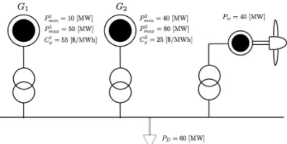
In order to motivate the discussion and provide some intuition on the cost benefits from allowing wind gener-ation to deviate from the available wind power output, four stylized examples are examined. These examples try to illustrate that, even though wind generation is not associated with any cost in the objective, it can still be beneficial to spill wind resources for a cost efficient al-location of conventional generation. Fig. 1 outlines the parameters for these examples.

In example 1, if the40MW of wind power are treated as a must-take resource, the total residual load that needs to be satisfied by conventional generation would be20MW. Due to the technical minimum40MW of gen-eratorG2, we need to use the expensiveG1, resulting in a1100 $/h cost of operation. If instead the output of the wind generator is adjusted at20MW,G1can be used and the cost drops to1000$/h.

In example 2, if wind power is a must-take resource, it can fully satisfy demand for time period2. A resid-ual load of20MW should be satisfied by conventional generation in periods1 and3. That, however, means that generatorG1must restart at period3and the startup costs are incurred twice, leading to a total cost of11000$ for the three periods. If, instead, 20MW of wind are spilled during the second time period, G1 can stay on and the total cost is now8500$. Note that this intuition could be extended for more time periods or for instances with more conventional generators.

(a) Example 1. The generator specifications in this case are minimum and maximum generation limits (Pmin,Pmax) and marginal costsCg. The available (maximum) wind power generation isPwand the load is

PD.

(b) Example 2. The generator specifications are the minimum genera-tion limit (Pmin), the startup costSgand the operating costC(P)as a function of the generation levelP. The available (maximum) wind power generationPwtand loadPDtare given for three consecutive time periods,t= 1,2,3.G1is assumed turned off at the beginning.

(c) Example 3. The generator specifications are minimum and maxi-mum generation limits (Pmin,Pmax), the startup costSg, the operating costC(P)as a function of the generation levelPand the ramping rate

RR. The available (maximum) wind power generation isPwand the load isPD. The generators are initially assumed turned off and we are only interested in the first time period.

C1 g= 4[k$/h] F12max= 10[pu] B12= 20[pu] G1 G2 F23max= 10[pu] B23= 20[pu] B13= 50[pu] F13max= 30[pu] Pw= 10[pu] PD= 40[pu] C2 g= 6[k$/h] 1 2 3

(d) Example 4. The system consists of three buses and three branches with susceptancesBand capacities Fmax _{as provided in the figure.}

The generator specifications are the marginal costsCg, the maximum available wind production isPwand the load isPD.

Figure 1: Small examples to illustrate potential benefits of wind power spilling.

In example 3, the goal is to satisfyN −1 security. More specifically, if any of the generators fail, we should be able to recover the lost generation within the next time unit (an hour is used here, but a smaller time reso-lution could be considered). GeneratorsG1andG2are identical and have a lower startup cost than generator G3, however their ramping rates are limited to60MW/h, whereasG3has a ramping rate of100MW/h. In the case where no wind spill is allowed, utilizing only the cheap generators does not yield a feasible solution, since as-suming they share the residual load of130MW by gen-erating65MW each, the ramping capabilities ofG1are not sufficient in caseG2fails (in case they share the load unevenly, the same problem arises if the highest gener-ating unit fails). So the costly generatorG3needs to be utilized, leading to a total cost of $12900. Now, if in-stead we dispatch the wind unit at40MW, by spilling 10MW of wind power, we can satisfy the residual load of140MW by evenly sharing betweenG1andG2, i.e. 70MW each. In case G2 suffers a fault, we can cover 60MW of its generation byG1and the remaining10MW we can obtain by ramping up the wind generation to its available output. For that, we exploit the fact that wind turbine controls allow for very fast ramping. The second dispatch amounts to a lower cost of $11200.

Finally, in example 4, a DC optimal power flow problem is solved to illustrate how allowing for flexible wind dispatch may lead to a more economical allocation by alleviating congestion. In the case where the10pu of wind power are treated as a must-take resource, in the optimum they all pass through branch2−3to satisfy the load of bus3, binding the phase angle difference be-tween buses 2and 3as well. That means the flow of branch2−3is at its capacity, so the flow on the line 1−2must be zero. Because of that, the phase of bus 1has to equal that of bus2and that constrains the flow on line1−3to25pu. We observe that both line1−2 and line1−3are not utilized close to their full capacity, whereas line2−3 is congested. Also,5pu of the load is satisfied by the expensive generatorG2, leading to a total cost of $130000/h. If we instead dispatch wind at 8pu, we can satisfy the load without using the expen-sive generator, by generating32pu withG1and the re-maining8pu through wind, leading to a lower total cost of $128000/h. The flows are in this caseP12 = 2pu, P23 = 10pu andP13 = 30pu, which also corresponds to a better utilization of the line capacities.

3.

Model Outline

The examples of the previous section constitute fa-vorable scenarios in which introducing flexible wind dispatch allows for a lower cost of operation, due to

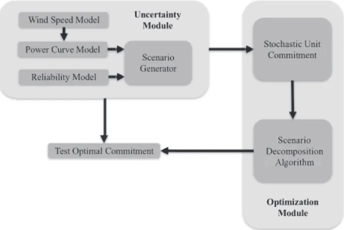
technical minima of conventional generation, efficient scheduling, ramping requirements or congestion. In or-der to make an argument for a more general case, how-ever, we need to consider a large set of scenarios, gen-erated based on a model of the underlying uncertainty of an actual system. For that purpose, the procedure de-picted in Fig. 2 is adopted. The developed model com-prises of two basic components, the Uncertainty Mod-ule and the the Optimization ModMod-ule. The Uncertainty Module tries to capture the underlying uncertainty of the system, which in our case is assumed to come from wind generation and line or generator faults. The mod-ule is trained based on a data set and then used to gen-erate scenarios whenever these are necessary. The Op-timization Module, on the other hand, takes as input a set of scenarios and solves a stochastic unit commitment problem, providing in its output a commitment sched-ule of the slow generators for the next day. The Opti-mization Module can be treated as a black box that a system operator uses to make the day ahead scheduling based on a set of available scenarios. Furthermore, it has two settings; in the first setting the optimization treats wind generation as a must-take resource, whereas in the second setting wind generation is allowed to dispatch at lower levels.

Based on these modules, the testing process is the following: Initially, the Uncertainty Module generates a set of scenarios. These scenarios are treated as the uncertainty information the system operator utilizes to make the scheduling decision. Based on this informa-tion, the Optimization Module makes one scheduling decision for each of two cases: the one in which wind is a must-take resource, and the one that it is not. In the final step, we wish to evaluate the difference between the costs associated with each case. To that end, we generate a new set of scenarios from the Uncertainty Module, rep-resenting possible actual realizations of the uncertainty the next day, and compare the expected costs of each of the two cases (Test Optimal Commitment Block).

3.1.

Uncertainty Module

The underlying uncertainty of the problem consid-ered consists of three main components: the wind model, the power curve model and the reliability model. The purpose of the wind model is to generate synthetic wind speed time series with hourly resolution, repre-sentative of the wind sites under consideration. Subse-quently, the power curve model takes as input the wind speed time series and outputs a wind power generation series for every wind site. Finally, the reliability model is a discrete (Bernoulli) distribution from where faults of lines and generators are drawn, as in [23].

&& &

"& !& &

Figure 2: General model outline. The Uncertainty Module generates scenarios to be used as input for the Optimization Module, which de-fines an optimal commitment. It also generates a new set of scenarios to test this optimal commitment.

3.1.1. Wind Speed Model A wind model that cap-tures the characteristics of wind speed from multiple wind sites is implemented. The approach follows the steps from [38], which builds upon work from [39] and [40]. The input data used to train the model are wind speed measurementsξgktrain, whereg∈GW indicates the different wind sites and k ∈ {1,2, ... Ttrain} indicates

theTtrain hourly measurements that are available at

ev-ery wind location. The goal is to train a model based on these measurements and then use it to generate ar-tificial wind series. The steps employed are divided in two phases; in the first one (Learning Phase) the model is trained using the time series data, whereas in the sec-ond one (Time Series Generation Phase) randomly gen-erated wind time series to be used in a Monte Carlo sim-ulation are created based on the model. The output of the process is a wind time seriesξgtssamplewithg ∈ GW (for the various wind sites),t ∈T (for the desired time steps of the SUC problem), ands∈S(different scenar-ios/samples used to capture the stochastic nature of the problem).

3.1.2. Power Curve Model For every site of wind generation an aggregate power curve that will provide an estimate of the wind power generation given the wind speed needs to be constructed. For that purpose, wind data and the corresponding wind power generations are used to train a power curve model. The power gener-ation data points come from an aggreggener-ation of multi-ple wind turbines in each site, with potentially differ-ent individual power curves and characteristics. There-fore, the use of the standard parametric power curve model of a single wind turbine to describe the wind

speed and power relationship [41] would not be a satis-factory approximation and a data driven non-parametric fit is more suitable. The model should also be able to capture the nonlinear behavior of the power curves, that is dependent on the wind speed operating point. For the aforementioned reasons, a local polynomial regression scheme is proposed.

More specifically, for every fixedg ∈GW the wind speed and wind power measurement dataξtrain

gk , Pgktrain

, k ∈ {1, . . . , Ttrain} are sorted (based on the

lexico-graphical ordering) inLgwind speed intervals[agi, bgi], wherei∈ {1,2, ...Lg}, with approximately equal num-ber of measurements, represented by a central wind speed pointcgi.We locally approximate the power curve mapping for this site with a polynomial of degreep, i.e. mgi(x) ≈ βgi0 +βgi1(x−cgi) +βgi2(x−cgi)2+ ... +βgip(x−cgi)p_{. The coefficients βgi}

0, . . . , βgip are trained for each interval based on a weighted least squares problem, where the weights are kernel functions of the distance of a point from the center of its interval. After an initial fit is obtained, the procedure in [33] is adopted to ensure the fit is robust to outliers.

Following that process, we feed the wind speed sam-ples ξgtssample, obtained by the wind speed model, to the trained power curve model, to obtain available wind power samplesPW gts, forg∈GW,t∈T,s∈S:

PW gts= Lg X i=1 mgi(ξsamplegts )I[agi,bgi](ξ sample gts ) (1)

3.2.

Optimization Module

3.2.1. Stochastic Unit Commitment The generat-ing units available to the system operator are divided into slow and fast, based on how long prior to opera-tion a commitment decision for that unit has to be made. The output of the SUC problem is the commitment of slow generating units. The challenge is that the commit-ment decision for slow units has to be made a day before operation, when the underlying uncertainty is still un-known, i.e. the commitment decisions (binary variables) for these units have to be the same across all scenarios (first stage variables). On the other hand, the other vari-ables of the problem, such as the commitment of fast generating units and the generation levels, are allowed to vary depending on which scenario of nature was real-ized (the decision for them is made with knowledge of the uncertainty), hence their value can be different for every scenario (second stage variables).

Our formulation is that of [23], adapted to explicitly model the flexibility of wind resources. The objective of

the SUC problem is minimizing the expected, over the different scenarios, operational costs (startup, minimum load and fuel costs), as well as the highly penalized load shed variables. Wind generation is not associated with any fuel costs in the objective. The only modification of our formulation, compared to the one in [23], is that wind will be treated as a must-take resource when an additional parameteriallinis set to 1. This is imposed

through the (additional) constraints:

pgts+pW Sgts=PW gts,∀g∈Gw,∀t∈T,∀s∈S,

(2a) pW Sgts≥0,∀g∈Gw,∀t∈T,∀s∈S, (2b)

pW Sgts≤(1−iallin)PW gts,∀g∈Gw,∀t∈T,∀s∈S,

(2c)

where the wind spillpW Sgts is set to zero ifiallin = 1

(forcing the wind generationpgtsto equal the available generationPW gts), or optimized to a value between zero and the maximum available wind productionPW gts, if iallin = 0. Note, however, that the policy adopted by

the operators when prioritizing wind generation is that they may still impose curtailments of wind generation, if the system feasibility is compromised. This corresponds to introducing constraint (2c) with a big-M penalty in the objective instead (which will lead to positive wind spill only in case enforcing (2c) as a hard constraint would cause infeasibility). The impact of the penalty is in that case subtracted from the objective cost reported, since the big-M has no physical meaning for the prob-lem costs.

3.2.2. Scenario Decomposition Algorithm The op-timization problem described previously has the form of a two-stage stochastic program. For concreteness, letx

be the vector of first stage variables, i.e. the slow gener-ator (binary) commitment. Letfs, fors∈S, be the set of (well defined) functions that, given the first stage vari-ables, yield the optimal cost for the second stage. That is, each evaluation offs(x)accounts for solving an

op-timization problem for scenarios∈Sand for first stage variablex. Then, the SUC can be reformulated:

minimize x∈X X s∈S πsfs(x) (3)

The binary nature of the first stage decisions in (3) al-lows the decomposition scheme proposed in [34] and elaborated in [35] to be employed in order to decom-pose the problem and reduce the computational burden. The form of decomposition utilized in this work is given in Fig. 3. The main body of the algorithm is divided

Initialization Phase t←0,U B← ∞,LB← −∞,wt s←0,∀s∈S,W ← ∅ Main Body repeat t←t+ 1,

Lower Bounding and Lagrangian Update Phase Solve scenario subproblems:

fors∈Sdo xt_s∈argmin

x_∈X\W

{fs(x) +xTwt_s−1}

end for

Update Lower Bound: LB←P_s∈Sπsfs(xts) Update objective weights: fors∈Sdo ˆ xt←P s∈Sπsxt_s wt_s←wt_s−1+ρ_t(xt_s−xˆt) end for

Upper Bounding and Cut Phase

Evaluate scenario solutions for Upper Bounds: fors∈Sdo

UBs←P_i∈Sπifi(xt_s) end for

Update Upper Bound: UB←min{UB,{UBs}s∈S} Exclude points tested: fors∈Sdo

W←W∪ {xt_s} end for

untilUB_UB−LB ≤eps

Figure 3: Decomposition scheme proposed in [34], adapted to solve the SUC problem. The Lower Bounding Phase involves solving smaller optimization problems than the original, since the scenario is fixed, whereas the Upper Bounding Phase involves smaller problems since the first stage and the scenario are fixed. As discussed in subsec-tion 3.2.2, not both phases are necessarily executed at every iterasubsec-tion.

into two phases, the Lower Bounding and Lagrangian Update Phase and the Upper Bounding Phase and Cut Phase. In the Lower Bounding Phase, we fix every sce-narios∈Sand solve for the optimal first stage decision given that scenario, over a spaceX\W. This yields|S|

scenario specific solutions for the first stage variables

xt_sat iterationt. In the first iteration, the setWis empty

and the penalty coefficientswt_sare zero, so we are

es-sentially solving|S|scenario subproblems without any interaction, i.e. we are solving the initial problem af-ter relaxing the non anticipativaty constraints. Since we are solving a relaxation, at least for the first iteration, we are guaranteed to get a lower bound on the optimal solution to (3). For the next iterations, it is still straight-forward [36] to show we get lower bounds for (3) solved in the restrained space of first stage variablesX\W.

Following that, the objective value penaltiesws for every scenarios ∈S are updated. These penalties aim to drive the scenario solutions together. Intuitively this is achieved in the following way: say that xis just an

one dimensionalxand for some iterationtwe have that the mean of the scenario specific solutions isxˆt_{. If for} some scenarios ∈ S, the scenario specific solutionxt s is away from the mean of the scenariosxˆt_(sayxt

s = 0 andxˆt _{= 0.9), we would like to penalize this deviation}

in the objective of the scenario subproblem the next time we iterate, at timet+1. So, at iterationt+1a term(xts−

ˆ

xt)xwill appear in the objective of scenarios, so that the new solutionxof the scenario will be driven towards the mean of the scenarios (in the arithmetic example, the penalty in the objective would be(0−0.9)x=−0.9x which will drivexto be1in the minimization, i.e. closer to the mean of the scenarios at the previous iteration).

In the Upper Bounding Phase of the algorithm, the

|S|scenario specific solutions for the first stage variables found during the previous phase are tested into the full problem. If feasible, each one of them yields an upper bound to (3). That way, we can possibly update the up-per bound and the first stage solution that yields it. We then add the points{xt

s}s∈S in the setW. Our objec-tive function value has already been calculated for all of these points, so we can exclude them from further con-sideration, except for the one that has yielded the best upper bound so far. That is, the execution of the Lower Bounding Phase for the next iteration should only con-sider points not inW. In practice, this is achieved by adding a global cut in the optimization problems solved in the first phase, for every point inWso as to cut off this particular point. More specifically, a “No-Good-Cut” is employed, i.e. a constraint of the form

xT(1−xt_s) + (1−x)Txt_s≥1, (4)

in order to cut off the point xt_s. The algorithm

it-erates until the Lower Bound (LB) and Upper Bound (UB) come close enough to satisfy the desired optimal-ity guarantee (eps).

To get some technical intuition for the algorithm, let us note that the Lower Bounding phase is essen-tially a step in a projected subgradient ascend scheme for the dual of (3) in the reduced spaceX\W, if the non-anticipativaty constraints are dualized. For a suit-able choice ofρtas a function of time, repeated evalua-tions of that phase would converge to the dual optimum. However, the dual optimum could be quite smaller than the primal optimum, due to the existence of a non zero duality gap, so we may never reach our desired optimal-ity guarantee. This is where the existence of the second phase of the algorithm becomes important: by expand-ing the setW, the duality gap between the primal in the spaceX\Wand its dual becomes smaller and, due to the finiteness ofX, we are guaranteed to eventually reach any predefined optimality guarantee threshold. In prac-tice, the objective penalties of the first phase are more useful at the beginning of the algorithm, since they lead the scenario specific solutions towards the same point

x, while the global cuts are more useful after the first

iterations, to reduce the optimality gap by cutting out points when the scenario solutions are similar to each

Type Units Capacity [MW]

Nuclear 2 4499 Gas 101 21781 Coal / Oil 3 /1 199 / 121 Dual Fuel 23 4679 Import 5 9931 Biomass 3 502 Geothermal 2 1073 Hydro 6 8613

Wind Low / Medium / High 5 1414 / 2121 / 2828 Table 1: Generator mix for the test system from [31, 39].

Wind Cost with/without Wind

Integration load shed Integration

Level [$M] [%]

Must Take Wind Spill Must Take Wind Spill

Low 8.23/8.23 8.23/8.23 13.2 13.0

Medium 6.98/6.98 6.95/6.95 19.8 18.9 High 16.09/7.27 6.11/6.11 26.3 23.4 Table 2: SUC solution evaluated on the test set: Mean cost of operation (without accounting for load shed) and wind penetration (percentage of mean, over the scenarios, wind energy over mean total generated energy).

other and the Lagrangian penalties do not offer signifi-cant improvements any more. So , the first phase of the algorithm is executed multiple times until a convergence indication is obtained. Following that, the second phase is executed and this process is repeated a few times.

4.

Simulation Results

We consider a reduced model of the Western Elec-tricity Coordinating Council (WECC) system [37] with 225buses,371lines and 130conventional generators. The same model is used in [39] and [31]. A typical win-ter weekday is simulated for three different integration cases: high, medium and low. High integration corre-sponds to26% wind energy penetration, the medium in-tegration corresponds to 19% penetration and the low integration to13%. The average load is28056MW, with a minimum of21438MW and a maximum of32300MW. The capacity of thermal generation is31281MW and the total generating capacity, not including wind resources, is 51402MW. The cost of load shedding is assumed $5000/MW-h and twice this value is assigned to the big-M relaxation of (2c). The generation mix is shown in

Wind Wind Load

Integration Spill Shed

Level [%] [%]

Must Take Wind Spill Must Take Wind Spill

Low 0 1.06 0 0

Medium 0 4.48 0 0

High 0.3 11.1 0.26 0

Table 3: SUC solution evaluated on the test set: Percentage of mean (over scenarios) wind spill over mean available generation and per-centage of mean loadshed over the total load.

Table 1.

The uncertainty model is trained based on data taken from [23]. These correspond to yearly time series of wind speeds and wind power generations with hourly resolution for five aggregate wind sites. The initial source was 2006 wind production data from the National Renewable Energy Laboratory database. A discrete dis-tribution is assumed for the reliability model, as in [39]. More specifically, a probability of generator failure of 1% and a probability of transmission line failure of 0.1% is assumed, independently.

All the simulations are performed on the Cab clus-ter of the Lawrence Livermore National Laboratory. For the simulations, Mosel 4.0.4 was used with Xpress [42]. Each excecution was parallelized in10nodes of the Cab cluster by utilizing the dedicated features of Mosel [43], allowing4threads per job and4jobs per node. The typ-ical values used forρtfor the decomposition algorithm wereρt∈[0.001,0.01], where the objective costs were normalized in $M. A2%optimality guarantee was set as a stopping criterion for the algorithm.

A total of160scenarios was generated and used as an input to the SUC problem. These scenarios represent the model available to the operator in the day ahead, based on which the optimization problem that defines the first stage variables is solved. A new set of160 sce-narios is generated, representing the actual realization of the uncertainty the day ahead. We explore two alterna-tive policies; one that allows for wind spill and one that assumes wind is a must-take resource, for the three in-tegration cases. The evaluation of the two policies, each one yielding a different first stage solution, is based on how they perform with the unseen scenarios.

The typical computational performance of the algo-rithm was as follows. The Lower Bounding phase would be executed until the LB would not improve more than 0.05%for two iterations. Note that, since the dual func-tion is non-differentiable, there is no guarantee that the subgradient will yield a descent direction, so this stop-ping criterion is merely a heuristic. Typically, the lower bounding phase would terminate within at most10-15 iterations. After that, the upper bounding phase would start by evaluating the function for the points that cor-respond to the best LB obtained. This process would be repeated typically2−3 times to obtain the desired optimality guarantee. It is important to note that, while the algorithm offers guaranteed convergence to any re-quired precision (as oposed to subgradient optimization schemes), it has a significant disadvantage for appli-cations that prioritize speed instead of accuracy. The Lower Bounding phase essentially has to solve mul-tiple subgradient optimization problems and the Up-per Bounding phase needs to evaluate the objective for

Must Take Wind Spill Dual Fuel Coal & Oil Gas Nuclear Dual Fuel Coal & Oil Gas Nuclear

Figure 4: Breakdown of total energy generation from conventional sources for the two policies examined in the high integration case. Note that the increased flexibility introduced by the wind allows for a higher utilization of the cheap generation from nuclear power plants.

Wind Spill Must Take

S

ce

n

ar

io

s

Cost [$M]

S

ce

n

ar

io

s

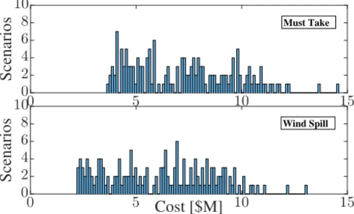
Figure 5: Histogram for the scenarios of stochastic unit commitment for the two policies in the high integration case. The variance of the scenario costs remains approximately the same (approximately equal to 6) for both policies, but the scenarios are spread around a lower mean for the wind spill case.

|S|points (which can be decomposed to solving |S|2 smaller mixed integer programs). The typical execution time was in the order of1−2hours, which is above the state-of-the art times reported in literature [32].

Tables 2 and 3 show the policy testing results. The fuel cost without load shedding is also provided. We observe that in the case of low and medium wind in-tegration, wind spilling does not result in a significant benefit. However, for high wind integration, the cost of operation is significantly lower when wind spill is al-lowed and load shed does not happen, whereas demand-ing the wind energy to be fully integrated leads to both an inefficient dispatch (high fuel costs) and an increased load shedding.

In Fig. 4, the reason of the more economical dis-patch can be seen: the extra flexibility enabled by op-timizing the wind output allows for a higher utilization of the cheap nuclear plants. Fig. 5 shows the

empiri-Must Take Wind Spill Total Cost

Startup Cost No Load Cost

Fuel Cost C o st [$ M ] 0 1 2 3 4 5 6 7 8 9 10

Figure 6: Comparison of the total cost, startup cost, no load cost and fuel cost for the two policies in the high integration case. Note that the bulk savings are obtained from the lower fuel costs due to the higher nuclear utilization.

cal distribution of the costs for the different scenarios of the stochastic unit commitment in the high integration case for the two policies. Finally, Fig. 6 shows the cost breakdown in the high integration case.

5.

Conclusions and Discussion

The main objective of this work is to convey that wind resources, and renewables in general, should be treated, to the extent possible, as any other resource for the unit commitment problem. Renewable integration is vital to achieve environmental goals, but it often com-petes with ensuring the secure and reliable operation of the grid due to the variability and stochasticity of the available wind power. However, current wind turbines are capable to control their output power setpoint within the limits allowed by wind availability. By exploiting this capability a safer and more economic grid operation can be ensured.

Regarding policy implications of adopting the pro-posed strategy, active wind spilling based on market op-erations can allow for a more efficient allocation (in-creased total welfare for the society), which could trans-late to benefits for the customers (in the form of reduced bills). The conventional generators will also be bene-fited, since they won’t have to fully carry the burden of grid security and reserve. Finally, even though adopt-ing this policy would mean an initial decrease in wind integration levels (since wind energy would be spilled), this strategy would enable a long term increase of re-newable integration, since part of the rere-newable inter-mittency problems would be resolved.

6.

Acknowledgments

Support for this work was received from the Ts-inghua Berkeley Shenzhen Institute, from ARO grant W911NF-17-1-0555, and from the Onassis Foundation. The authors would like to thank Deepak Rajan and the Lawrence Livermore National Laboratory that enabled us to parallelize our computations, Ignacio Aravena and Anthony Papavasiliou for their useful comments, and FICO for providing licenses for Xpress Optimizer.

References

[1] “Flexible Resources Help Renewables,” California ISO, 2016. [Online]. Available: https://www.caiso. com/Documents/FlexibleResourcesHelpRenewables\

FastFacts.pdf

[2] “Curtailment Fast Facts,” California ISO, 2017. [On-line]. Available: https://www.caiso.com/Documents/ CurtailmentFastFacts.pdf

[3] European Union, “Directive 2009/28/EC of the Euro-pean Parliament and of the Council of 23 April 2009 on the promotion of the use of energy from renewable sources and amending and subsequently repealing Di-rectives 2001/77/EC and 2003/30/EC,”Official Journal of the European Union, vol. 5, p. 2009, 2009.

[4] P. Moutis, S. A. Papathanassiou, and N. D. Hatziar-gyriou, “Improved load-frequency control contribution of variable speed variable pitch wind generators,” Re-newable Energy, vol. 48, pp. 514–523, 2012.

[5] S. I. Nanou, G. N. Patsakis, and S. A. Papathanassiou, “Assessment of communication-independent grid code compatibility solutions for VSC–HVDC connected off-shore wind farms,” Electric Power Systems Research, vol. 121, pp. 38–51, 2015.

[6] S. Fink, C. Mudd, K. Porter, and B. Morgenstern, “Wind energy curtailment case studies,”NREL subcontract re-port, NREL/SR-550, vol. 46716, 2009.

[7] L. Bird, J. Cochran, and X. Wang, “Wind and so-lar energy curtailment: experience and practices in the United States,”US National Renewable Energy Labora-tory, NREL/TP-6A20-60983, p. 3, 2014.

[8] S. Liu, “Phase I.A. Stochastic Study Testimony of Dr. Shucheng Liu on behalf of the California Independent System Operator Corporation,” 11 2014.

[9] K. Meeusen, “Phase I.A. Stochastic Study Testimony of Dr. Karl Meeusen on behalf of the California Indepen-dent System Operator Corporation,” 11 2014.

[10] A. Solomon, D. M. Kammen, and D. Callaway, “The role of large-scale energy storage design and dispatch in the power grid: a study of very high grid penetration of vari-able renewvari-able resources,”Applied Energy, vol. 134, pp. 75–89, 2014.

[11] D. J. Burke and M. J. O’Malley, “Factors influencing wind energy curtailment,” IEEE Transactions on Sus-tainable Energy, vol. 2, no. 2, pp. 185–193, 2011. [12] G. Oggioni, F. H. Murphy, and Y. Smeers, “Evaluating

the impacts of priority dispatch in the European electric-ity market,” Energy Economics, vol. 42, pp. 183–200, 2014.

[13] E. Ela and D. Edelson, “Participation of wind power in LMP-based energy markets,”IEEE Transactions on Sus-tainable Energy, vol. 3, no. 4, pp. 777–783, 2012. [14] L. Deng, B. F. Hobbs, and P. Renson, “What is the cost

of negative bidding by wind? A unit commitment analy-sis of cost and emissions,”IEEE Transactions on Power Systems, vol. 30, no. 4, pp. 1805–1814, 2015.

[15] L. S. Vargas, G. Bustos-Turu, and F. Larra´ın, “Wind power curtailment and energy storage in transmission congestion management considering power plants ramp rates,” IEEE Transactions on Power Systems, vol. 30, no. 5, pp. 2498–2506, 2015.

[16] R. Golden and B. Paulos, “Curtailment of Renewable En-ergy in California and Beyond,”The Electricity Journal, vol. 28, no. 6, pp. 36–50, 2015.

[17] L. Kane and G. W. Ault, “Evaluation of wind power cur-tailment in active network management schemes,”IEEE Transactions on Power Systems, vol. 30, no. 2, pp. 672– 679, 2015.

[18] M. Hedayati-Mehdiabadi, J. Zhang, and K. W. Hedman, “Wind power dispatch margin for flexible energy and re-serve scheduling with increased wind generation,”IEEE Transactions on Sustainable Energy, vol. 6, no. 4, pp. 1543–1552, 2015.

[19] M. Hedayati-Mehdiabadi, K. W. Hedman, and J. Zhang, “Reserve Policy Optimization for Scheduling Wind En-ergy and Reserve,” IEEE Transactions on Power Sys-tems, vol. 33, no. 1, pp. 19–31, 2018.

[20] M. Carri´on and J. M. Arroyo, “A computationally ef-ficient mixed-integer linear formulation for the thermal unit commitment problem,”IEEE Transactions on Power Systems, vol. 21, no. 3, pp. 1371–1378, 2006.

[21] P. Damcı-Kurt, S. K¨uc¸¨ukyavuz, D. Rajan, and A. Atamt¨urk, “A polyhedral study of production ramp-ing,”Mathematical Programming, vol. 158, no. 1-2, pp. 175–205, 2016.

[22] S. Fattahi, M. Ashraphijuo, J. Lavaei, and A. Atamt¨urk, “Conic relaxations of the unit commitment problem,”

Energy, vol. 134, pp. 1079–1095, 2017.

[23] A. Papavasiliou and S. S. Oren, “Multiarea stochastic unit commitment for high wind penetration in a transmis-sion constrained network,”Operations Research, vol. 61, no. 3, pp. 578–592, 2013.

[24] S. Takriti, J. R. Birge, and E. Long, “A stochastic model for the unit commitment problem,”IEEE Transactions on Power Systems, vol. 11, no. 3, pp. 1497–1508, 1996. [25] P. Carpentier, G. Gohen, J.-C. Culioli, and A. Renaud,

“Stochastic optimization of unit commitment: a new de-composition framework,”IEEE Transactions on Power Systems, vol. 11, no. 2, pp. 1067–1073, 1996.

[26] A. Tuohy, P. Meibom, E. Denny, and M. O’Malley, “Unit commitment for systems with significant wind penetra-tion,” IEEE Transactions on power systems, vol. 24, no. 2, pp. 592–601, 2009.

[27] J. Deane, G. Drayton, and B. ´O. Gallach´oir, “The impact of sub-hourly modelling in power systems with signif-icant levels of renewable generation,” Applied Energy, vol. 113, pp. 152–158, 2014.

[28] M. E. Khodayar, M. Shahidehpour, and L. Wu, “Enhanc-ing the dispatchability of variable wind generation by co-ordination with pumped-storage hydro units in stochastic power systems,”IEEE Transactions on Power Systems, vol. 28, no. 3, pp. 2808–2818, 2013.

[29] K. Cheung, D. Gade, C. Silva-Monroy, S. M. Ryan, J.-P. Watson, R. J.-B. Wets, and D. L. Woodruff, “Toward scalable stochastic unit commitment,” Energy Systems, vol. 6, no. 3, pp. 417–438, 2015.

[30] K. Kim and V. M. Zavala, “Algorithmic innovations and software for the dual decomposition method applied to stochastic mixed-integer programs,”Mathematical Pro-gramming Computation, pp. 1–42, 2017.

[31] A. Papavasiliou, S. S. Oren, and B. Rountree, “Ap-plying high performance computing to transmission-constrained stochastic unit commitment for renewable energy integration,” IEEE Transactions on Power Sys-tems, vol. 30, no. 3, pp. 1109–1120, 2015.

[32] I. Aravena and A. Papavasiliou, “An Asynchronous Dis-tributed Algorithm for solving Stochastic Unit Com-mitment,” Universit´e catholique de Louvain, Center for Operations Research and Econometrics (CORE), Tech. Rep., 2016.

[33] W. S. Cleveland, “Robust locally weighted regression and smoothing scatterplots,” Journal of the American statistical association, vol. 74, no. 368, pp. 829–836, 1979.

[34] S. Ahmed, “A scenario decomposition algorithm for 0– 1 stochastic programs,” Operations Research Letters, vol. 41, no. 6, pp. 565–569, 2013.

[35] K. Ryan, D. Rajan, and S. Ahmed, “Scenario decom-position for 0-1 stochastic programs: Improvements and asynchronous implementation,” inParallel and Dis-tributed Processing Symposium Workshops, 2016 IEEE International. IEEE, 2016, pp. 722–729.

[36] D. Gade, G. Hackebeil, S. M. Ryan, P. Watson, R. J.-B. Wets, and D. L. Woodruff, “Obtaining lower bounds from the progressive hedging algorithm for stochastic mixed-integer programs,” Mathematical Programming, vol. 157, no. 1, pp. 47–67, 2016.

[37] N.-P. Yu, C.-C. Liu, and J. Price, “Evaluation of market rules using a multi-agent system method,”IEEE Trans-actions on Power Systems, vol. 25, no. 1, pp. 470–479, 2010.

[38] D. D. Le, G. Gross, and A. Berizzi, “Probabilistic Mod-eling of Multisite Wind Farm Production for Scenario-Based Applications,” Sustainable Energy, IEEE Trans-actions on, vol. 6, no. 3, pp. 748–758, 2015.

[39] A. Papavasiliou and S. S. Oren, “Stochastic modeling of multi-area wind production,” in12th International Con-ference on Probabilistic Methods Applied to Power Sys-tems, 2012.

[40] J. M. Morales, R. Minguez, and A. J. Conejo, “A method-ology to generate statistically dependent wind speed sce-narios,” Applied Energy, vol. 87, no. 3, pp. 843–855, 2010.

[41] M. Lydia, S. S. Kumar, A. I. Selvakumar, and G. E. P. Kumar, “A comprehensive review on wind turbine power curve modeling techniques,”Renewable and Sustainable Energy Reviews, vol. 30, pp. 452–460, 2014.

[42] C. Gu´eret, C. Prins, and M. Sevaux, “Applications of op-timization with Xpress-MP,”contract, p. 00034, 1999. [43] Y. Colombani and S. Heipcke, “Multiple models and

par-allel solving with Mosel, February 2014,”Avalaible at: http://community. fico. com/docs/DOC-1141.