Publications
11-2016
Bridge damage detection using spatiotemporal
patterns extracted from dense sensor network
Chao Liu
Iowa State University, [email protected]
Yongqiang Gong
Iowa State University, [email protected]
Simon Laflamme
Iowa State University, [email protected]
See next page for additional authors
Follow this and additional works at:http://lib.dr.iastate.edu/ccee_pubs
Part of theAcoustics, Dynamics, and Controls Commons,Civil Engineering Commons, Electro-Mechanical Systems Commons,Environmental Engineering Commons, and theOther Mechanical Engineering Commons
The complete bibliographic information for this item can be found athttp://lib.dr.iastate.edu/ ccee_pubs/98. For information on how to cite this item, please visithttp://lib.dr.iastate.edu/ howtocite.html.
This Article is brought to you for free and open access by the Civil, Construction and Environmental Engineering at Iowa State University Digital Repository. It has been accepted for inclusion in Civil, Construction and Environmental Engineering Publications by an authorized administrator of Iowa State University Digital Repository. For more information, please [email protected].
Chao Liu, Yongqiang Gong, Simon Laflamme, Brent M. Phares, and Soumik Sarkar
Bridge damage detection using spatiotemporal
patterns extracted from dense sensor network
Chao Liu1, Yongqiang Gong2, Simon Laflamme2, Brent Phares2, Soumik
Sarkar1
1Department of Mechanical Engineering,
2Department of Civil, Construction and Environmental Engineering,
Iowa State University, Ames, IA 50011, USA
E-mail: [email protected]
Abstract. The alarmingly degrading state of transportation infrastructures combined with their key societal and economic importance calls for automatic condition assessment methods to facilitate smart management of maintenance and repairs. With the advent of ubiquitous sensing and communication capabilities, scalable data-driven approaches is of great interest, as it can utilize large volume of streaming data without requiring detailed physical models that can be inaccurate and computationally expensive to run. Properly designed, a data-driven methodology could enable fast and automatic evaluation of infrastructures, discovery of causal dependencies among various sub-system dynamic responses, and decision making with uncertainties and lack of labeled data. In this work, a spatiotemporal pattern network (STPN) strategy built on symbolic dynamic filtering (SDF) is proposed to explore spatiotemporal behaviors in a bridge network. Data from strain gauges installed on two bridges are generated using finite element simulation for three types of sensor networks from a density perspective (dense, nominal, sparse). Causal relationships among spatially distributed strain data streams are extracted and analyzed for vehicle identification and detection, and for localization of structural degradation in bridges. Multiple case studies show significant capabilities of the proposed approach in: (i) capturing spatiotemporal features to discover causality between bridges (geographically close), (ii) robustness to noise in data for feature extraction, (iii) detecting and localizing damage via comparison of bridge responses to similar vehicle loads, and (iv) implementing real-time health monitoring and decision making work flow for bridge networks. Also, the results demonstrate increased sensitivity in detecting damages and higher reliability in quantifying the damage level with increase in sensor network density.
1. Introduction
The number of civil structures with critical aging concerns is becoming significantly large and the cost of repairing and upgrading them is estimated at $2.2 trillion USD [1, 2, 3]. In the United States alone, the average age of the 607,380 bridges is 42 years, and the Federal Highway Administration (FHWA) estimated that we would need to invest $76
for any errors or omissions in this version of the manuscript or any version derived from it. The Version of Record is available online at doi: 10.1088/1361-6501/28/1/014011. Posted with permission.
billion USD to repair deficient bridges. This and other recent infrastructure failures have raised serious concerns about the structural integrity of the aging and deteriorating civil infrastructures around the world, about the inefficiency, ineffectiveness and non-uniformity of visual inspection, which is still the prevalent method for infrastructure inspection, and about societies’ readiness to respond, to mitigate, to forecast, to manage, and to minimize the risks associated with aging infrastructures.
A solution is to automate the condition assessment process, also known as structural health monitoring (SHM). SHM of civil infrastructures (e.g., bridges, wind turbines, buildings, nuclear structures, etc.) is a difficult task due to the large geometries under inspection. A fundamental challenge is the lack of scalability of existing sensing solution, due to economic and/or technical challenges associated with off-the-shelf sensors. For example, resistive foil gauges are widely used to monitor existing cracks, but are geometrically too small to be capable of detecting a new damage of a large area within an acceptable level of probability [4]. It follows that, to enable damage localization on over a large system, one needs to deploy sensor networks of given density to achieve the damage localization resolution of interest.
Several sensor networks have been proposed in literature, based on fiber optics [5, 6] and piezoelectric [7, 8] technologies for instance. These networks have been used for structural health monitoring, displacement prediction of aerospace structures, and control of smart systems [9, 10, 11]. However, their applications are typically sparse because of their prohibitive costs [12]. Nevertheless, if properly designed, they have the possibility to detect, localize, and quantify damage at a given resolution.
Recent advances in nanotechnologies and conductive polymers have led to the engineering of low-cost dense sensor networks (DSNs), de facto enabling high resolution capabilities. For example, DSNs can be constructed from a network of conductive particles forming a continuous set of sensors within a structural component [13, 14], and from large-area electronics that mimic biologic skin [15, 16, 4, 17]. Dense network applications have been demonstrated using arrays of tactile cells [18], using a 36-sensor array of resistive heating elements on a flexible polyimide film to measure shear stress topography and flow separation on the leading edge of a delta-wing structure [19], and using large sensing sheets of strain gauges with embedded processors for crack detection and localization [20, 16].
Despite the great promise of these technologies at being deployed over large-scale systems in the future, algorithms and tools leveraging DSNs for SHM need to be developed. This includes the concept of system of systems, where a set of DSNs is interconnected in a given network to provide measurements enabling SHM of the network itself. Of interest are transportation infrastructure networks. While the condition assessment research community is extremely active in developing tools and methodologies enabling automatic evaluation of transportation infrastructure, the vast majority of the effort is on the input-model-output perspective, at a single system level (e.g., a structure equipped with sensors). The problem is not typically approached in terms of systems of systems. There has been some
research conducted in the evaluation of infrastructure systems resiliency, that investigated infrastructures as an interconnected system. These studies mainly studied the impact of that a bridge closure would have on an entire network, and did not consider the integration of sensor data. See references [21, 22, 23, 24] for instance. There is an important opportunity in agglomerating local networks of sensors for improving the condition assessment process, which constitute a system of systems, also termed complex system.
In this paper, we propose to leverage the unique spatial properties of bridges in a transportation network to evaluate their conditions in a complex system framework. Bridges constitute critical connection points in the transportation system. In addition, adjacent bridges in a system have typically very similar vehicle loads, weather conditions, and geotechnical conditions. In the spatial and temporal space, the behavior of the bridges are relative, noted as causality in graph theory. Discovering the spatiotemporal features in the bridge system is beneficial in detecting potential changes in structural integrity, and improving the efficiency and accuracy of bridge inspections by providing the inspectors with useful data for guidance and identification of potential problems, instead of uniquely relying on visual procedures and the inspector’s judgment.
The spatiotemporal discoveries will be made through the comparison of intrinsic geometry of data sets. This idea has been previously applied in the field of SHM. For instance, [25] used a multivariate attractor-based approach to detect the presence and magnitude of damage in structures through the investigation of the response’s phase-space constructed by a time delayed embedding. Ref. [26] compared an attractor constructed from the undamaged state to predict structural response, and identified damage as a change in the prediction error. In [27], the dynamic system is divided in subsystems to cope with nonlinearities, and the time series response of each subsystem is analyzed. The study in [28] proposed to analyze nonlinear time series using a multivariate autoregressive approach in order to detect damage under varying operational and environmental conditions. Ref. [29] used a combined state-space embedding strategy and singular value decomposition to detect structural damage. Refs [30, 31, 17, 32] used a diffusion map-based approach for detection of anomaly in dynamic systems.
Other multivariate statistical techniques for processing quantities of data obtained from DSNs have been proposed in the field. Studies reported in [33] applied a multivariate statistical technique to analyze the data acquired from a continuously monitored long-span arch bridge using the real-time identified natural frequencies as sensitive features. Ubertini et al. [34] conducted a multivariate statistical analysis criterion on a bell-tower in Italy to investigate its dynamic characteristics under wind loading. Research on multivariate statistical methods (clustering analysis, autoregressive with moving average models) were also applied in the field of structural health monitoring [35, 36].
Recently symbolic dynamic filtering (SDF) [37] based techniques have been proposed for pattern discovery in spatiotemporally distributed systems that enable establishing and representing causal interactions among the subsystems [38]. SDF, as a data-driven dynamical
system modeling technique, has advantages in describing different types of data with a uniform symbolic representation as well as low time and memory complexity. Symbolic time-series features captured by SDF can be used in the formation of a spatiotemporal pattern network (STPN) as reported in recent studies [39, 40].
Contributions: This work explores spatiotemporal behaviors in a network of bridges from a condition monitoring perspective. Data from dense sensor networks of strain gauges from the bridges are simulated using finite element method, and analyzed using STPN. The causality (the causes and the effects) information of strain data is applied for damage detection and isolation, as the causality includes critical features of the dynamical system health and has great potential in detecting damage and reasoning failure scenarios. Case studies are conducted based on strain data of two adjacent bridges simulated with various vehicle (e.g., truck) loads as well as different damage levels. Performance comparisons for different damage levels, among a DSN, a nominal sensor network (NSN), and a sparse sensor network (SSN) are presented to validate the advantages of a DSN.
The organization of the paper is as follows: In section 2, preliminaries on STPN and metrics for STPN are presented. While section 3 describes the bridge modeling and data generation procedures, frameworks for vehicle matching and damage detection are presented in section 4. In section 5, we show the results of vehicle matching and damage detection. Based on that, we form a real-time health monitoring and decision making framework. The paper is summarized and concluded along with future research directions in section 6.
2. Background and preliminaries
2.1. Spatiotemporal pattern network
SDF has been recently shown to be extremely effective for extracting key textures from time-series data [37]. The main idea is that a symbol sequence (i.e., discretized time-series) emanated from a process can be approximated as a Markov chain of order D (also called depth), named as D-Markov machine [38] that captures the essential behavior of the underlying process.
The discretization or symbolization process is noted as partitioning [37]. Let X denote a set of partitioning functions, X : X(t) → S, that transforms a general dynamic system (time series X(t)) into a symbol sequence S using an alphabet set Σ. Various approaches are proposed in the literature, depending on different objective functions, such as uniform partitioning (UP), maximally bijective discretization (MBD)[41], statistically similar discretization (SSD) [42], and maximum entropy partitioning (MEP). This study uses simple uniform partitioning.
TheD-Markov machine is essentially a probabilistic finite state automaton (PFSA) that can be described by states (representing various parts of the data space) and probabilistic transitions among them that can be learnt from data. Related definitions of deterministic finite state automaton (DFSA), PFSA, D-Markov machine, xD-Markov machine and the
learning schemes can be found in [38].
With this setup, a spatiotemporal pattern network (STPN) is defined below [40].
Definition. A PFSA based STPN is a 4-tuple WD ≡ (Qa,Σb,Πab,Λab): (a, b denote nodes of the STPN)
(i) Qa ={q
1, q2,· · ·, q|Qa|} is the state set corresponding to symbol sequences Sa;
(ii) Σb ={σ
0,· · ·, σ|Σb|−1} is the alphabet set of symbol sequence Sb;
(iii) Πab is the symbol generation matrix of size |Qa| × |Σb|, the ijth element of Πab denotes the probability of finding the symbolσj in the symbol stringsb while making a transition from the state qi in the symbol sequence Sa; while self-symbol generation matrices are called atomic patterns (APs) i.e., when a = b, cross-symbol generation matrices are called relational patterns (RPs) i.e., when a6=b.
(iv) Λab denotes a metric that can represent the importance of the learnt pattern (or degree of causality) for a→b which is a function of Πab.
2.2. Information based metric for causality
Based on the definition of STPN, patterns discovered between the vertices can be applied to interpret the causality via proper metrics. Information based criteria are usually applied, e.g., transfer entropy [43] and mutual information [38, 44]. This work applies mutual information for representing Λab of the patterns (APs & RPs). Definition of mutual information for Λab is as follows.
Λab ,Iab =I(qk+1b ;qak+1) =H(qbk+1)−H(qbk+1|qka) (1) where, Iab is the mutual information of pattern (a, b), H is the conditional entropy defined as follows, H(qk+1b ) = − Qb X i=1 P(qbk+1 =i) log2P(qkb =i) H(qk+1b |qak) = Qa X i=1 P(qak =i)H(qbk+1|qka =i) H(qk+1b |qak =i) =− Qb X j=1 P(qk+1b =j|qak =i)·log2P(qk+1b =j|qka=i)
Detailed description of mutual information based causality metric in the context of APs and RPs can be found in [38].
2.3. Similarity metric for STPNs
As a kind of graphical model, STPN can adopt metric for estimating similarity of graphs. However, most of the metrics in graphs are defined with the binary values (0/1) of the vertices/edges [45], and they do not consider edge weights (represented by mutual information in this work) between vertices. To incorporate such mutual information based degree of causality among nodes or vertices in estimating similarity between two STPNs, this study applies a structural similarity (SSIM) metric. SSIM was first proposed and applied in image processing, and it was demonstrated to be more effective in image quality assessment [46] and feature extraction [47].
Considering full connections (APs & RPs) between nnodes in an STPN, a matrix with causality metric n×n is formed. Treating the causality matrix as n vectors in an image (similar to the definition of SSIM in image quality assessment [46]), SSIM can be applied to estimate the similarity between two causality matrices in two STPNs. The general form of the structure similarity index [46] between two vectors xand y is
S(x, y) = 2µxµy+C1 µ2 x+µ2y +C1 α 2σxσy +C2 σ2 x+σ2y+C2 β σxy +C3 σxσy+C3 γ , (2)
where µx, µy are the means of x and y respectively, σx2, σy2 are the variances of x and y respectively, σxy is the cross covariance of x and y, parameters α, β and γ are used to adjust the relative importance of the three components, with α > 0, β > 0 and γ >0; C1,
C2, C3 are the constants to avoid instability when the denominators are very close to zero,
C1 = (K1L)2, C2 = (K2L)2, C3 =C2/2, K1,K2 and Lare constants.
3. Data generation using Finite Element Method
3.1. Bridge models
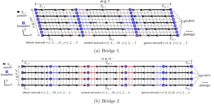
Two adjacent steel-concrete composite bridges located in West Des Moines, Iowa, were simulated. Bridge 1 is 200 ft long and 38 ft wide with 3 spans, 5 longitudinal girders and 2 traffic lanes, while bridge 2 is 540 ft long and 28.5 ft wide with 5 spans, 4 longitudinal girders and 1 traffic lane. Planar-level finite element models of these two bridges were generated using 688 linear beam elements, 328 quadrilateral shell elements, 381 linear beam elements, and 162 quadrilateral shell elements in the finite element software WinGen [48]. As shown in Fig. 1, the girders, stringers and floor beams were modeled using elastic beam elements, whereas the concrete deck was idealized using quadrilateral shell elements. The number of beam and shell elements of both bridges is shown in Table 1. Steel girder and stringer sections near piers were modeled as non-composite beams (red and blue elements in Fig. 1), while those in the middle spans and side piers were modeled as composite ones (black elements in Fig. 1). Initial sections and material properties were assigned to all elements to match the design of two bridges. The boundary conditions were also idealized using rotational spring elements with appropriate initial stiffness [49].
(a) Bridge 1
(b) Bridge 2
Figure 1. Modeling the bridges using Finite Element Method. Three sensor network are defined with stain gages, including nominal sensor network (NSN, corresponding to practical sensor installment), dense sensor network (DSN) and sparse sensor network (SSN).
For each bridge, three types of sensor network are defined, noted as DSN, NSN and SSN, where NSN follows a typical sensor installment, DSN installs more sensors along the traveling direction, and SSN reduces sensors along the traveling direction. The sensors of the three sensor networks are shown in Fig. 1.
Table 1. Number of beam and shell elements for the bridge models.
Item Bridge 1 Bridge 2
Beam elements - Girders 200 216
Beam elements - Stringers 160
-Beam elements - Floor 328 165
Shell elements 320 162
Under damage conditions, the damage was assigned by reducing the moment of inertia of given girder elements, shown in Fig. 1. Damage levels of 5%, 10% and 20% were assigned by reducing the moment of inertia by 5%, 10% and 20%, respectively.
A total of 20 trucks were randomly selected from the truck library in WinGen and individually driven (in the simulations) on bridges. Trucks were simulated as static loads. Strain data was collected and analyzed under nominal condition and damaged conditions. 3.2. Headway simulation
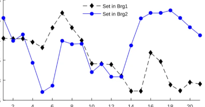
In each simulation, trucks are driven over the bridge with a given time separating the lead truck and the following truck, termed headway. Headway is generated from traffic modeling
data found in [50].
Random-walk Metropolis-Hastings sampler is applied to generate the headway set, and an example is shown in Fig. 2. Using the simulated headway, strain data in each 20-truck set is generated, as shown in Fig. 3. When there is no truck on the bridge, the stain is taken as 0 (as only truck loading is considered in this work). When there is more than one truck on the bridge simultaneously, strain histories are added linearly. Bridge 2 contains more data set that includes simultaneous trucks given its longer length relative to bridge 1.
Truck ID 2 4 6 8 10 12 14 16 18 20 Headway (s) 2.5 3 3.5 4 4.5 5 Set in Brg1 Set in Brg2
Figure 2. Example of generated headway.
Time (s) 0 10 20 30 40 50 60 Strain (10 -6) 0 50 100 (a) Bridge 1 Time (s) 0 10 20 30 40 50 60 Strain (10 -6) 0 50 100 (b) Bridge 2
Figure 3. Simulated strain data at mid-span for both bridges with 20 trucks.
3.3. Noise addition
In order to evaluate the robustness of the algorithm to noise in sensor data, noise is generated using a uniform distribution, and the amplitude is taken as 5% of the maximum of the measurements. The noisy strain data (regarding the strain data in Fig. 3) is shown in Fig. 4.
Time (s) 0 10 20 30 40 50 60 Strain (10 -6) 0 50 100 (a) Bridge 1 Time (s) 0 10 20 30 40 50 60 Strain (10 -6) 0 50 100 (b) Bridge 2
Figure 4. Strain of two bridges after noise added. The same spans are shown as in Fig. 3.
4. Damage detection framework for bridge network with spatiotemporal pattern network
4.1. Formation of STPN in vehicle matching between bridges
In this work, vehicle matching is referred to a successful identification of a vehicle driving sequence. Vehicle matching is critical to conduct the spatiotemporal study of structural behaviors on a network of bridges (Section 5.3), as they are taken as constant inputs. Note, although vehicle matching is beneficial in improving damage detection accuracy, it is not strictly required, as one may conduct spatiotemporal studies assuming that a given vehicle sequence remains constant between two adjacent bridges (no passing, no vehicle exiting/entering - more details provided in Section 5.3).
To implement vehicle matching, causality between sensors from the two bridges is applied to extract the pair-wise features. The basic idea is that under nominal condition, the causal relationship between the two sets of strain responses is unique when the same vehicle passes on the bridges one after another. In other words, the strain in the first bridge can be applied to reliably predict the strain in the second bridge, given that the same vehicle is passing on the bridges one after another.
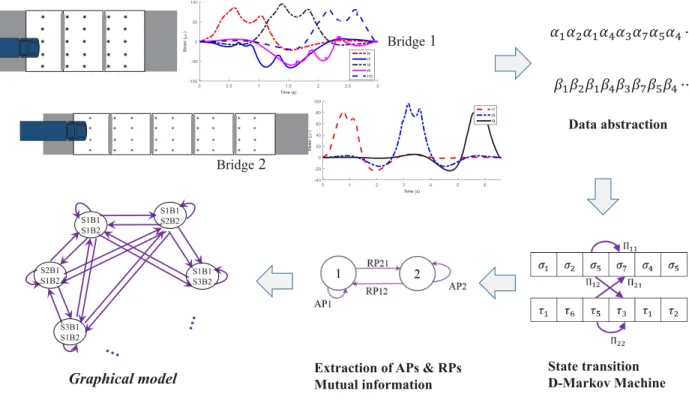
The STPN-based vehicle matching procedure is illustrated in Fig. 5. The algorithm for vehicle matching is as follows.
Algorithm 1. Vehicle matching in bridges. 1 Input: Strain data{Xn
i, i∈m}in bridgenwith vehicle set (IDsm={1,2,· · ·, M}). Strain data ˜Xn
i with current vehicle (IDi) passing by. 2 Output: Matched vehicle set ˜m.
3 Modeling and learning.
4 Obtain symbol sequences S with strain data X using the alphabet set Σ. Here, partitioning is implemented in two dimensional space, the strain from the sensor in bridge 1 is noted as the first dimension, and the strain from the sensor in bridge 2 is noted as the second dimension. The dimensions ofS areg×h, representing number of sensors in bridge 1 and bridge 2 respectively.
5 Form the state sequences Qwith symbol sequences S using depth Dof PFSA. 6 for all a∈g, b∈h, do
Bridge1 Bridge2 Data abstraction ߙଵߙଶߙଵߙସߙଷߙߙହߙସڮ ߚଵߚଶߚଵߚସߚଷߚߚହߚସڮ State transition D-Markov Machine Extraction of APs & RPs
Mutual information Graphical model S1B1 S1B2 S1B1 S3B2 S2B1 S1B2 S3B1 S1B2 S1B1 S2B2
Figure 5. Framework in formation of spatiotemporal pattern network and graphical model for vehicle matching.
7 Compute the state transition matrix Πab with xD-Markov machine. 8 end
9 for all a∈g, b∈h, do
10 Compute the mutual information Λab with Eq. 1. 11 end
12 Repeat step 4-11, obtain the mutual information set {Λg×h}M×M. 13 Truck Matching.
14 Obtain symbol sequences ˜S with strain data ˜Xusing the alphabet set Σ. 15 Form the state sequences ˜Qwith symbol sequences ˜S using depth Dof PFSA. 16 Compute the state transition matrix ˜Π with xD-Markov machine.
17 Obtain the mutual information ˜Λ with Eq. 1. 18 for all i∈m,j ∈m, do
19 Compute the similarity between ˜Λ and {Λg×h}ij, i is the vehicle ID passing bridge 1,j is the vehicle ID passing bridge 2.
20 end
4.2. Formation of STPN for damage detection
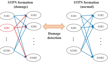
Bridges in the network are geographically close, the vehicle loads are therefore similar. Under this assumption, the causality between the bridges is relatively stable and consistent. If the damage is induced in one bridge in some aspect, e.g., span damage due to an external effect, the causality between the damaged bridge and other bridges would change.
S1B1
…
S2B1 S36B2 S2B2 S25B1 S1B2. .
.
STPN formation (normal) S1B1…
S2B1 S36B2 S2B2 S25B1 S1B2. .
.
STPN formation (damage) Damage detectionFigure 6. Formation of STPNs for damage detection in two bridges.
To detect the damage of the bridge in the above situation, this work applies STPN in estimating the variation of causality between the bridges. The steps in data abstraction, state transition formation, and extraction of causality are similar to Section 4.1, the damage detection approach is shown in Fig. 6. Two STPNs are formed in the nominal condition and anomaly (damage) condition, respectively, and the variation of the causality is compared pattern by pattern. The expectation is that the damaged location will present increased strain and this can be captured by causality metric in STPN. The damage detection approach also provides a view for damage localization as the sensor presenting the variation of causality indicates the damage position where the sensor is installed.
The algorithm for damage detection is as follows.
Algorithm 2. Damage detection on two adjacent bridges (with the assumption that the trucks passing the two bridges are similar).
1 Input: Strain data{Xn
i, i∈m}in bridgenwith vehicle set (IDsm={1,2,· · ·, M}). Strain data with damage{X˜n
i} in bridgen with vehicle set (IDsm={1,2,· · ·, M}). 2 Output: Damage level and location.
3 Modeling in nominal condition.
4 Obtain symbol sequences S with strain data X using the alphabet set Σ. Here, symbolization is implemented in one dimensional space regarding time series generated from a single sensor. The numbers of sensors in bridge 1 and bridge 2 are U and V, respectively.
6 for all a∈U,b ∈V, do
7 Compute the state transition matrix Πab with xD-Markov machine. 8 end
9 for all a∈U,b ∈V, do
10 Compute the mutual information Λab with Eq. 1. 11 end
12 Modeling in anomalous condition.
13 Obtain symbol sequences ˜S with strain data ˜X using the alphabet set Σ. Here, symbolization is implemented in one dimensional space regarding time series generated from a single sensor. The numbers of sensors in bridge 1 and bridge 2 are U and V, respectively.
14 Form the state sequences ˜Qwith symbol sequences ˜S using depth Dof PFSA. 15 for all a∈U,b ∈V, do
16 Compute the state transition matrix ˜Πab with xD-Markov machine. 17 end
18 for all a∈U,b ∈V, do
19 Compute the mutual information ˜Λab with Eq. 1. 20 end
21 Inference.
22 Compute the difference between{Λ˜}and{Λ}, to obtain the damage level and location. It should be noted that in this work, the algorithms for vehicle matching and damage detection are based on two bridges. However, the approach can be easily extended to the bridge network with multiple bridges, where the relations in the bridge network can be considered pairwise. STPNs formed in vehicle matching and damage detection are different in structure, further work will pursue a unified framework in processing feature extraction for both vehicle matching and damage detection.
5. Results and discussions
5.1. Vehicle matching
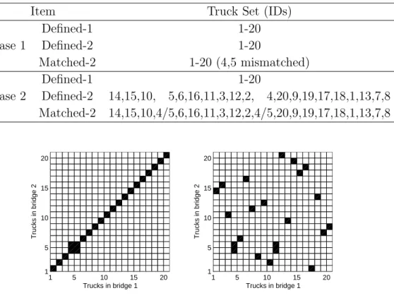
Vehicle matching is carried out in two cases: (1) the order of the two truck sets are identical, with the assumption that there is no passing of trucks between the bridges, and (2) the orders are different, and the passing of trucks is random. The vehicle matching results are shown in Fig. 7. The IDs in defined orders and matched orders are listed in Table. 2.
In the two cases, the trucks 4 and 5 are mismatched. The reason is that the weights and dimensions of the two trucks are similar, and the strain caused by the two trucks are very close (as shown in Fig. 8).
The case presented above utilizes noiseless data. The accuracy in truck matching may decrease in diverse noise levels and future work will focus on the truck matching algorithm for noisy data sets.
Table 2. Truck matching results in two cases. Defined-1 and Defined-2 are orders of trucks on bridge 1 and bridge 2 respectively (treated as ground truth), Matched-2 is order of trucks on bridge 2 (matching results).
Item Truck Set (IDs)
Case 1 Defined-1 1-20 Defined-2 1-20 Matched-2 1-20 (4,5 mismatched) Case 2 Defined-1 1-20 Defined-2 14,15,10, 5,6,16,11,3,12,2, 4,20,9,19,17,18,1,13,7,8 Matched-2 14,15,10,4/5,6,16,11,3,12,2,4/5,20,9,19,17,18,1,13,7,8 1 5 10 15 20 1 5 10 15 20 Trucks in bridge 1 Trucks in bridge 2
(a) Case 1, trucks in same order
1 5 10 15 20 1 5 10 15 20 Trucks in bridge 1 Trucks in bridge 2
(b) Case 2, trucks in different order
Figure 7. Truck matching results. The block in black shows the matching result and the detected truck IDs are in x-axis and y-axis respectively.
5.2. Damage detection
Damage detection is implemented with the same truck sets used in the above section, where the damage data in bridge 1 is applied. With the nominal and damage data in the bridge 1, the patterns of the STPNs are computed and the variation between them is used for damage detection. Here, as the bridges are adjacent, we assume more of the vehicles passing by the bridges are similar. The same vehicle set is used to generate the stain data in bridge 1 and bridge 2 (nominal and damage cases respectively). For the damage cases, damage is injected in bridge 1 using the approach in Section 3.1.
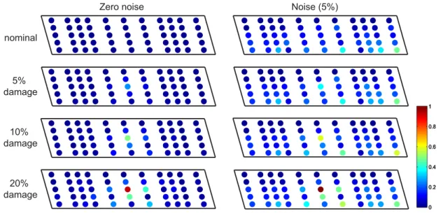
The damage detection results are shown in Fig. 9. Anomaly score of each sensor is defined as the difference of the mutual information between damaged cases ( ˜Λab) and the nominal case with zero noise (Λab), noted as F da = PNb=1b |Λ˜ab−Λab|, a = 1,2,· · ·, Na,
b = 1,2,· · ·, Nb, Na and Nb are the numbers of sensors in bridges 1 and 2 respectively. In damage cases, the sensor in red shows significant difference of mutual information and indicates high anomaly score in this location. Compared with Fig. 1 (a), the sensor with high anomaly score is consistent with the damage location. This feature can be used for fault
0 50 100 150 200 250 300 −50 0 50 100 150 Position Strain Truck 1 Truck 4 Truck 5 Position 40 50 60 70 80 90 Strain 40 60 80 100 120 Truck 1 Truck 4 Truck 5
(a) Local strain of bridge 1
0 100 200 300 400 500 600 −20 0 20 40 60 Position Strain Truck 1 Truck 4 Truck 5 Position 240 260 280 300 320 340 Strain 0 10 20 30 40 50 60 Truck 1 Truck 4 Truck 5
(b) Local strain of bridge 2
Figure 8. Strain in mismatched trucks (trucks 4 & 5, unit in 10−6).
Zero noise Noise (5%)
nominal 5% damage 10% damage 20% damage
Figure 9. Damage detection results using DSN. The color at each sensor shows the anomaly score, which is obtained using the differences of the mutual information (computed via Eq.1) between damaged cases and nominal case (zero noise, top-left corner). The anomaly score are normalized by the maximal value in 20% damage case to make results comparable, while this causes loss of significance in 5% damage case.
isolation. The results show that the fault can be located in all of the three damage cases in zero-noise data (shown in the left panel). For the noisy data, fault can be located in 20% damage case as the fault position presents maximal anomaly. In the 10% and 5% damage cases, although there are anomaly detected in the fault position, some other locations also indicate deviation, as of noise influence. With the results, the subset of the sensors showing anomaly can be applied in downselecting the potential fault location.
Table 3. Damage detection results– DSN.
Case Anomaly score Alarm status (p-value)
Zero noise Nominal 0 0 5% damage 0.34 1 10% damage 0.60 1 20% damage 1.18 1 Noise Nominal 1.69 0 5% damage 1.81 1 (0.019) 10% damage 1.85 1 (0.0028) 20% damage 2.28 1 (1.04e-20)
Table 4. Damage detection results– NSN.
Case Anomaly score Alarm status (p-value)
Zero noise Nominal 0 0 5% damage 0.08 1 10% damage 0.14 1 20% damage 0.29 1 Noise (5%) Nominal 0.27 0 5% damage 0.32 1 (0.0090) 10% damage 0.32 1 (0.034) 20% damage 0.46 1 (1.32e-10)
To evaluate the health status of the bridge, anomaly scores of sensors are used to compute the anomaly score of the bridge F dsa, defined as F dsa =PNa
a=1F da, and the results are listed in Tables 3-5 in DSN, NSN, SSN, respectively.
Anomaly scores in all sensors consist of much information of the damage in diverse locations of the bridge. To apply this information in decision making, hypothesis testing (two-samplet-test) is carried out, to determine if the anomaly score in damage case is same as the nominal condition. In two-samplet-test, the null hypothesis is that two datasets come from independent random samples from normal distributions with equal means and equal but unknown variances, and an outcomeh= 1 means that the test rejects the null hypothesis at the 5% significance level, and 0 otherwise. Therefore,h = 1 indicates the testing samples are
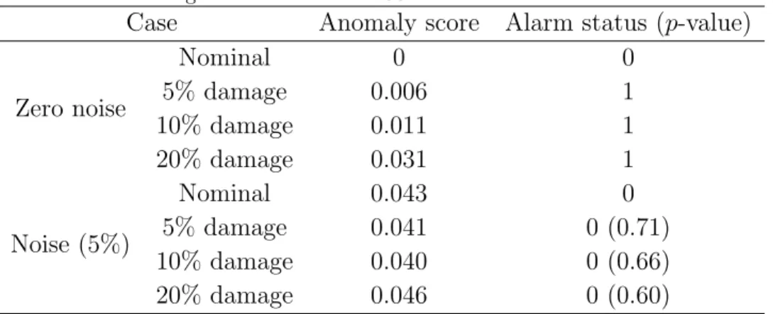
Table 5. Damage detection results– SSN.
Case Anomaly score Alarm status (p-value)
Zero noise Nominal 0 0 5% damage 0.006 1 10% damage 0.011 1 20% damage 0.031 1 Noise (5%) Nominal 0.043 0 5% damage 0.041 0 (0.71) 10% damage 0.040 0 (0.66) 20% damage 0.046 0 (0.60)
different from the nominal condition, and can be identified as damage/anomaly/fault. Using two-sample t-test, the results of damage detection (alarm status) are listed in Tables 3-5.
The results show that, using DSN and NSN, damage can be correctly detected in 5%, 10% and 20% levels, where thep-values are small which suggests a high decision confidence. However, damage can not be detected by SSN in all of the three cases (using noisy data), where the p-value decreases with damage level and it means that the confidence decreases. Note that damage detection in zero-noise cases is simple as anomaly scores are easily computed (anomaly scores in nominal condition are all 0), and damage can be detected in all cases with DSN, NSN, and SSN.
To further compare the performance of DSN, NSN, and SSN, the increase of anomaly score is computed based on the anomaly score in the nominal case, and the results are shown in Fig. 10. DSN obtains a more significant increase of anomaly score in three damage levels, and is more sensitive to detect small damage, which is beneficial for early detection. Also, anomaly score increase for DSN is monotonous with increasing damage level, while NSN and SSN do not necessarily demonstrate such a property. As a result, DSN is also more reliable to quantify the damage level.
5.3. Real-time decision making via integrating vehicle matching and damage detection Vehicle matching and damage detection (detection and isolation) are validated in the previous sections. In this section, a real-time decision making process flowchart integrating vehicle matching, damage detection, and fault isolation is presented, as shown in Fig. 11. The bridges are adjacent, and it is more likely that the same vehicle passes by. Therefore, same vehicle assumption is used in the first step. The four steps are as follows:
(i) Vehicle matching using the same vehicle assumption (Algorithm 1). If matched, obtain the result (a)-same vehicle, healthy bridge. Otherwise, go to (ii).
(ii) Damage detection (Algorithm 2). If the damage is detected, go to (iii). Otherwise, implement vehicle matching in different vehicles and obtain the result (b)-vehicle pair and healthy bridge.
Damage (%) 0 5 10 15 20 Anomaly (%) 0 5 10 15 20 25 30 35 DSN NSN SSN
Figure 10. Relationship between damage degree and anomaly in DSN, NSN, and SSN.
(iii) Fault isolation. Localize the sensors at/close to the damaged location(s) (Algorithm 2), then go to (iv).
(iv) Vehicle matching. Implement vehicle matching with the updated sensors, obtain the results (c)-same vehicle, damage bridge, or (d)-vehicle pair, damage bridge.
The test results show that vehicle matching fails when there’s damage on bridge 2 (top-right corner in Fig. 11). With damage detection and fault isolation implemented, sensors close to the damage locations are excluded, and the re-matching works (case (c) and (d) in Fig. 11).
It should be noted that, for damage detection and decision making, we need a given number of data points to make the transition matrix (used in computing the probability of transition between states of variables) statistically stable. It follows that the quality of the detection increases with the number of vehicles driving on the bridge. In practical applications, we would expect a large number of vehicle (much larger than the 20 vehicles used in the simulations) resulting in a good convergence of the condition assessment process. 5.4. Discussions
This work applied simulation data in truck matching and damage detection in bridge network, and the simulation data is generated by finite element method based on two existing bridges. Noise is added with a predefined amplitude and uniform distribution. Further analysis is being carried out to analyze typical characteristics of strain gauges used in bridge monitoring to get more field-like signals. Also, the trucks used in this work are randomly picked; further work is being implemented in generating more data sets to cover typical dimensions and weights of diverse trucks.
Regarding understanding the causal relations between bridges in terms of vehicle matching and damage detection, this work applied spatiotemporal pattern network with the simulation data in two bridges. The results show that the proposed approach can effectively
(b) Different vehicles, healthy bridge
Vehicle matching (Same vehicle assumption)
Matched vehicle pair, healthy bridge Matched Damage detection Fault isolation Excluding sensors at damage location(s) Yes No Vehicle matching (Different vehicles) Same vehicle Matched vehicle pair,
Damaged bridge Matched vehicle pair,
healthy bridge
Matched vehicle pair, Damaged bridge
Different vehicles
(a) Same vehicle, healthy bridge (d) Different vehicles, Damaged bridge (c) Same vehicle, Damaged bridge Not matched Vehicle matching
Figure 11. Real-time decision making via integrating vehicle matching, damage detection and fault isolation.
discover the behavior of the strain responses with different trucks passing bridges, and detect the abnormal damage in a bridge by estimating the variation of the causal relationship between two bridges geographically close. With the ability in processing a large-scale dataset, the proposed approach can be applied in complex networks with dense sensor networks, and the application provides a novel view in damage detection via exploring causality between bridge network. Note that because the STPN is built on symbolic dynamics, the partitioning process of STPN is adaptive in diverse data types [40], including continuous and discrete data. In particular, vibration-based data (from accelerometers, for instance) could be used with the STPN framework.
Note that no denoising technique is applied in this work, and the proposed approach naturally handles the noisy data and captures the features in damage cases.
A real-time decision making process is formulated via integration of vehicle matching and damage detection. The test results show that the process is capable of obtaining vehicle matching and damage detection together. Note, due to the computational efficiency of STPN, the decision process can be used in real-time health monitoring and decision making applications.
6. Conclusions
With spatiotemporal pattern network, this work conducted vehicle matching and damage detection for a small bridge network composed of two adjacent bridges, both equipped with dense sensor networks of strain gauges. The proposed approach is designed for processing large-scale dataset in a bridge network (from a network of dense sensor networks), and the results show the advantages of the proposed approach in: (i) capturing spatiotemporal features to discover causality between bridges (geographically close), (ii) handling noise in data for feature extraction, (iii) detecting and localizing damage via comparing the behaviors in the bridge network, and (iv) implementing real-time health monitoring and decision making for bridge network. Also, the results show that dense sensor network is more sensitive in detecting damage and more reliable to quantify the damage level.
The proposed approach for the damage detection is based on the data generated by multiple trucks. The current application is implemented in two bridges with one-span damage case. The further work will pursue: (i) damage detection in multiple cases with diverse damage levels, (ii) detecting damage with more realistic noise levels as a function of the sensor type and environment conditions, and (iii) including more variables to model the relation between bridge network, e.g., weather, traffic pattern, structure parameters.
Acknowledgments
This paper is based upon research partially supported by the National Science Foundation under Grant No. CNS-1464279 and Grant No. CMMI-1463252. Any opinions, findings, and conclusions or recommendations expressed in this material are those of the authors and do not necessarily reflect the views of the National Science Foundation.
References
[1] Brownjohn J 2007 Philosophical Transactions of the Royal Society A: Mathematical, Physical and Engineering Sciences 365589–622
[2] Harms T, Sedigh S and Bastianini F 2010Instrumentation & Measurement Magazine, IEEE 1314–18 [3] Simon J, Bracci J and Gardoni P 2010 Journal of Structural Engineering 1361273–1281
[4] Kharroub S, Laflamme S, Song C, Qiao D, Phares B and Li J 2015 Smart Materials and Structures 24
[5] L´opez-Higuera J, Rodriguez Cobo L, Quintela Incera A and Cobo A 2011Lightwave Technology, Journal of 29587–608
[6] Costa B and Figueiras J 2012Engineering Structures 44271–280
[7] Yu L, Giurgiutiu V, Ziehl P, Ozevin D and Pollock P 2010 Steel bridge fatigue crack detection with piezoelectric wafer active sensorsSPIE Smart Structures and Materials+ Nondestructive Evaluation and Health Monitoring (International Society for Optics and Photonics) pp 76471Y–76471Y
[8] Gresil M, Yu L, Shen Y and Giurgiutiu V 2013 Smart Structures and Systems 121738–1584 [9] Ko W L, Richards W and Tran V T 2007NASA Technical Reports
[10] Gherlone M, Cerracchio P, Mattone M, Di Sciuva M and Tessler A 2011Dynamic shape reconstruction of three-dimensional frame structures using the inverse finite element method (National Aeronautics and Space Administration, Langley Research Center)
[11] Derkevorkian A, Masri S F, Alvarenga J, Boussalis H, Bakalyar J and Richards W L 2013AIAA journal
512231–2240
[12] Liu W, Tang B and Jiang Y 2010Renewable Energy 351414–1418
[13] DAlessandro A, Ubertini F, Materazzi A L, Laflamme S and Porfiri M 2015Structural Health Monitoring
14137–147
[14] Ubertini F, Materazzi A L, D‘Alessandro A and Laflamme S 2014Engineering Structures 60265–275 [15] Laflamme S, Saleem H S, Vasan B K, Geiger R L, Chen D, Kessler M R and Rajan K 2013Mechatronics,
IEEE/ASME Transactions on 181647–1654
[16] Tung S, Yao Y and Glisic B 2014Measurement Science and Technology 25 075602
[17] Wu J, Song C, Saleem H S, Downey A and Laflamme S 2015Measurement Science and Technology 26
055103 URLhttp://stacks.iop.org/0957-0233/26/i=5/a=055103
[18] Lee H K, Chang S I and Yoon E 2006Microelectromechanical Systems, Journal of 151681–1686 [19] Xu Y, Jiang F, Newbern S, Huang A, Ho C M and Tai Y C 2003 Sensors and Actuators A: Physical
105321–329
[20] Hu Y, Rieutort-Louis W S, Sanz-Robinson J, Huang L, Glisic B, Sturm J C, Wagner S, Verma Net al. 2014Solid-State Circuits, IEEE Journal of 49 513–523
[21] Bocchini P and Frangopol D M 2011Journal of Engineering Mechanics 139760–769 [22] Soy Transportation Coalition 2013
[23] Saydam D, Bocchini P and Frangopol D M 2013Engineering Structures 54221–233
[24] Fitzsimmons E J, Mulinazzi T E and Schrock S D 2014 Economic impact of closing structurally deficient or functionaly obsolete bridges on very low-volume roadsTransportation Research Board 93rd Annual Meeting pp 14–4486
[25] Moniz L, Nichols J, Nichols C, Seaver M, Trickey S, Todd M, Pecora L and Virgin L 2005Journal of Sound and Vibration 283295–310
[26] Overbey L, Olson C and Todd M 2007Smart Materials and Structures 161621–1638
[27] Monroig E 2009Detection of Changes in Dynamical Systems by Nonlinear Time Series Analysis Ph.D. thesis University of Tokyo
[28] Figueiredo E, Todd M, Farrar C and Flynn E 2010 International Journal of Engineering Science 48
822–834
[29] Liu G, Mao Z, Todd M D and Huang Z 2013Structural Health Monitoring 131–142
[30] Rabin N and Averbuch A 2010 Detection of anomaly trends in dynamically evolving systems. AAAI Fall Symposium: Manifold Learning and Its Applications
[31] Huang Y, Zha X F, Lee J and Liu C 2013Mechanical Systems and Signal Processing34 277–297 [32] Jiang Y, Li Z, Zhang C, Hu C and Peng Z 2016Measurement Science and Technology 27065103 [33] Comanducci G, Magalh˜aes F, Ubertini F and Cunha ´A 2016Structural Health Monitoring 15505–524 [34] Ubertini F, Comanducci G and Cavalagli N 2016Structural Health Monitoring 15438–457
[35] Santos J P, Cr´emona C, Orcesi A D and Silveira P 2013Engineering Structures 56273–285 [36] Pakzad S N and Fenves G L 2009Journal of structural engineering 135863–872
[38] Sarkar S, Sarkar S, Virani N, Ray A and Yasar M 2014Frontiers in Robotics and AI 116
[39] Jiang Z and Sarkar S 2015 Understanding wind turbine turbine interactions using spatiotemporal pattern networkProceedings of ASME Dynamics Systems and Control Conference
[40] Liu C, Ghosal S, Jiang Z and Sarkar S 2016 An unsupervised spatiotemporal graphical modeling approach to anomaly detection in distributed cps Proceedings of the International Conference of Cyber-Physical Systems, (Vienna, Austria)
[41] Sarkar S, Srivastav A and Shashanka M 2013 Maximally bijective discretization for data-driven modeling of complex systemsAmerican Control Conference (ACC), 2013 (IEEE) pp 2674–2679
[42] Sarkar S and Srivastav A 2016 Signal Processing 125 156 – 170 ISSN 0165-1684 URL
http://www.sciencedirect.com/science/article/pii/S0165168416000359
[43] Wibral M, Rahm B, Rieder M, Lindner M, Vicente R and Kaiser J 2011 Progress in biophysics and molecular biology 10580–97
[44] Solo V 2008 On causality and mutual informationDecision and Control, 2008. CDC 2008. 47th IEEE Conference on (IEEE) pp 4939–4944
[45] Papadimitriou P, Dasdan A and Garcia-Molina H 2010Journal of Internet Services and Applications1
19–30
[46] Wang Z, Bovik A C, Sheikh H R and Simoncelli E P 2004Image Processing, IEEE Transactions on 13
600–612
[47] Liu C, Jiang D and Yang W 2014Expert Systems with Applications 413585–3595 [48] Bridge Diagnostics Inc 2001 User’s manual: WinGen
[49] Seo J, Phares B, Lu P, Wipf T and Dahlberg J 2013Engineering Structures 46569–580
[50] Houchin A, Dong J, Hawkins N and Knickerbocker S 2015 Measurement and analysis of heterogenous vehicle following behavior on urban freeways: Time headways and standstill distances Intelligent Transportation Systems (ITSC), 2015 IEEE 18th International Conference on (IEEE) pp 888–893