Gerhard Tutz, Shahla Ramzan
Improved Methods for the Imputation of Missing
Data by Nearest Neighbor Methods
Technical Report Number 172, 2014 Department of Statistics
University of Munich
Improved Methods for the Imputation of Missing
Data by Nearest Neighbor Methods
Gerhard Tutz and Shahla Ramzan
Ludwig-Maximilians-Universit¨at M¨unchen
Akademiestraße 1, 80799 M¨unchen
October 13, 2014
Abstract
Missing data is an important issue in almost all fields of quantitative re-search. A nonparametric procedure that has been shown to be useful is the nearest neighbor imputation method. We suggest a weighted nearest neighbor
imputation method based on Lq-distances. The weighted method is shown to
have smaller imputation error than available NN estimates. In addition we con-sider weighted neighbor imputation methods that use selected distances. The careful selection of distances that carry information on the missing values yields an imputation tool that outperforms competing nearest neighbor methods dis-tinctly. Simulation studies show that the suggested weighted imputation with selection of distances provides the smallest imputation error, in particular when the number of predictors is large. In addition, the selected procedure is applied to real data from different fields.
Keywords: kernel function, weighted nearest neighbors, cross-validation,
weighted imputation, MCAR,
1 Introduction
Missing data have always been a challenging topic for researchers. Ignoring all the missing cases is not a good strategy to deal with missing values. In the lit-erature many techniques have been suggested since the 1980s to impute missing data, see, for example, Little and Rubin (1987), Schafer (2010). Broadly speak-ing, the methods for filling the incomplete data matrix can be divided into two main categories; single imputation and multiple imputation (Little and Rubin (1987)). A well known and computationally simple method for imputation of missing data is mean substitution. A disadvantage of the method is that the
cor-relation structure among the predictors is ignored. An alternative is thenearest
neighbors approach, which uses the observations in the neighborhood to impute
missing values. Nearest neighbors as a nonparametric concept in discrimination dates back to Fix and Hodges (1951). The approach has been successfully used to impute data in gene expression (Troyanskaya et al. (2001), Atkeson et al. (1997), Hastie et al. (1999)), machine learning (Batista and Monard (2002)), medicine (Waljee et al. (2013)), forestry (Eskelson et al. (2009), Hudak et al. (2008)), and compositional data (Hron et al. (2010)) etc.
An important aspect in missing data imputation is the pattern of missing values because the selection of an imputation procedure is determined by this pattern. Little and Rubin (1987) defined three categories of missing data; miss-ing completely at random (MCAR), missmiss-ing at random (MAR), and not missmiss-ing at random (NMAR). Missing completely at random (MCAR) refers to the data in which the probability of a particular missing values does not depend on the variable itself or any other variable in the data set (Little and Rubin (1987), Allison (2001)). Most imputation methods assume the data to be at least MAR, if not MCAR, and so does the nearest neighbor method.
Hastie et al. (1999) proposed to use weights based on the Euclidean
dis-tance for the selection of the nearest neighbors. A comparison of k nearest
neighbor imputation (KNNimpute) with mean imputation and singular value decomposition (SVD) techniques for gene expression data was given by Troy-anskaya et al. (2001). The results of their simulation studies showed that the method performs well when compared to mean imputation and singular value decomposition (SVD) approaches, see also Troyanskaya et al. (2003). In a com-parative study of single imputation methods, Malarvizhi and Thanamani (2012) found that median or standard deviation substitution perform better than mean substitution. Therefore replacement of a missing value with simple average is not an efficient method. A further comparison of KNNimpute with mean, OLS and PLS imputation methods for imputation in microarray data was given by Nguyen et al. (2004). The findings of the study showed that KNNimpute per-forms well.
Several alternative procedures have been proposed that rely on the basic concept to impute values by building averages over qualifying neighbors, see, for example Ouyang et al. (2004), Kim et al. (2004), Sehgal et al. (2005), Scheel et al. (2005). Liew et al. (2011) and Moorthy et al. (2014) reviewed the available methods and algorithms for the imputation of missing values with a focus on
gene expression data. Johansson and Hakkinen (2006) proposedWeNNI, which
utilizes continuous weights in the nearest neighbors imputation procedure. Bø et al. (2004) and Wasito and Mirkin (2005) proposed a nearest neighbors pro-cedure with a modification based on the least square principle. Other variants include local least squares (LLSimpute) by Kim et al. (2005), sequential local least square (SLLSimpute) by Zhang et al. (2008) and iterative local least square (ILLSimpute) by Cai et al. (2006).
A drawback of NN methods is that their performance depends on k. For
example, KNNimpute typically performs well when k is between 5 to 10, but
the performance deteriorates for larger k (Yoon et al. (2007)). We propose a
localized approach to missing data imputation that uses a weighted average
of nearest neighbors using Lq distances. For the high-dimensional case, we
propose a new distance that explicitly uses the correlation among variables. The proposed method automatically selects the relevant variables that contribute to
the distance and thus does not depend onk.
The paper is organized as follows: in Section 2 the Lq distance is used to
define a weighted imputation estimate. In a simulation study the weighted approach is compared to the unweighted approach. In Section 3, the weighted imputation with selection of predictors is introduced and compared to alternative imputation techniques. In Section 4 several applications to real data sets are given.
2 Weighted Neighbors
When using nearest neighbors to impute data several choices have to be made. In particular one has to define what nearest neighbors are, that means, how they are computed and which distance measures are used. Then one has to choose how these nearest neighbors are used to obtain an imputed value. These choices to be made are considered in the following sections.
2.1 Distances and Computation of Nearest Neighbors
Let n observations on p covariates be collected. The corresponding n×p data
matrix is given by X = (xis),where xis denotes the ith observation of the sth
variable. LetO= (ois) denote the correspondingn×pmatrix of dummies with
entries
ois =
1 ifxis was observed
0 for missing value.
Distances between two observations xi and xj, which are represented by rows
in the data matrix, can be computed by using the Lq-metric for the observed
data. Then one uses the distances
dq(xi,xj) = [ 1 mij p X s=1 |xis−xjs|qI(ois= 1)I(ojs= 1)]1/q, (1)
wheremij =Pps=1I(ois= 1)I(ojs= 1) denotes the number of valid components
in the computation of distances. The indicator function I(a), which is used in
the definition, has the value 1, if ais true and 0 otherwise. Thus, computation
of distances does not use all the components of the vectors. It uses only those components for which observations in both vectors are available. The actually
used components in the computation of neighbors is given byCij ={s:I(ois=
1)I(ojs= 1) = 1}. The distances are used to define the nearest neighbors when
imputing a specific value. It should be noted that the number of components that
are used varies over the sample becauseCij depends on the specific observation
for which imputations are to be made.
Similar concepts to define distances and therefore nearest neighbors were used by Hastie et al. (1999), Troyanskaya et al. (2001), Myrtveit et al. (2001)
and Kim et al. (2005). They used the Euclidean distance,q= 2. Other
alterna-tives to compute distances in gene expression studies were by use of the Pearson correlation (Dudoit et al. (2002), Bø et al. (2004)) and covariance estimate (Se-hgal et al. (2005)).
2.2 Imputation Procedure
Imputation for Fixed Number of Neighbors
Let us consider imputation forxi in components, that is,ois= 0. The
imputa-tion estimate forxi is based on theknearest neighbors in the reduced data. One
determines the knearest neighbors from the corresponding (˜n×p)-dimensional
reduced data set X˜ = (xij, ois = 1) obtaining
x(1), . . . ,x(k) with d(xi,x(1))≤ · · · ≤d(xi,x(k)),
where xT(j) = (x(j)1, . . . , x(j)p) denotes the jth nearest neighbor. Then the
ˆ xis = 1 k k X j=1 x(j)s (2)
Thus the missing value in the sth component of observation vector xi is
replaced by the average of the corresponding values of the knearest neighbors.
The accuracy of the method is mainly determined by the number of neighbors that are used. Simple rules use a fixed number of neighbors that are chosen by the experimenter. However, it is advantageous to consider the number of neighbors as a tuning parameter that is chosen in a data-driven way, for example by cross-validation (see next section).
Imputation by Weighting
A disadvantage of the imputation based on the k nearest neighbors is that the
value of the first nearest neighbor has the same importance as thekth nearest
neighbor. A more appropriate method uses weights that account for the distance of the observations. We consider a weighted average of neighbors based on
distances that are determined by kernel functions. The weighted imputation
estimate considered here has the form
ˆ xis = k X j=1 w(xi,x(j))x(j)s (3) with weights w(xi,xj) =K(d(xi,xj)/λ)/ k X l=1 K(d(xi,xj)/λ), (4)
where K(.) is a kernel function (for example tricube, Gaussian) and λ is a
tuning parameter. For small λ, the weights are decreasing very strongly with
the distance, whereas for λ→ ∞, one uses equal weights for all neighbors. To
makeλthe crucial tuning parameter one should use a large number of potential
neighbors. In the extreme case, if one uses k = ˜n, the window-width λ is the
only tuning parameter.
Alternative weights were used by Troyanskaya et al. (2001). They used the
weighted average over the knearest neighbors based on the Euclidean distance
with the weights determined by the inverse of the Euclidean distance.
2.3 Choice of Tuning Parameters by Cross-validation
An important issue in weighted nearest neighbors imputation techniques is the
selection of the tuning parameter λ. One option is to use the same method
that is in common use when selecting the optimal number of nearest neighbors
k, namely cross-validation, see, for example,Dudoit et al. (2002). Also some
R packages provide cross-validation as a tool to choose the optimal number of nearest neighbors (Waljee et al. (2013)). The concept is to artificially delete some values in the data matrix and compute the mean squared error (MSE) or mean absolute error (MAE) for the artificially deleted data. Then one chooses the value for which MSE or MAE takes the minimal value.
In our approach we generate completely at random (MCAR) m∗ artificially
missing values from the available data{xis:ois = 1}. LetX∗ denote the n×p
artificially missing values ({x∗is :o∗is= 0}). Then the mean absolute error (MAE) for these observations is defined by
MAE(X∗) = 1
m∗
X
xis:o∗is=0
|x∗is−x∗is(imputed)|. (5)
This procedure is repeated R times yielding the averaged value
MAECV= 1 R R X r=1 MAE(X∗r),
where X∗r denotes the matrix with both types of missing values in the rth
replication. In the same way the cross-validated mean square error (MSE) is computed by using MSE(X∗) = 1 m∗ X xis:o∗is=0 (x∗is−x∗is(imputed))2 (6) yielding MSECV.
The cross-validation is done in the following way:
1. For a specific value ofλ;
a. Artificially deletem∗ value/s in the data matrix.
b. Impute these missing values and calculate MSE or MAE.
c. Repeat a and b, R times for example, R = 100 depending upon data,
to find MSECVor MAECV.
2. Repeat steps a-c for all values of λ, and choose the one with minimum
MSECV or MAECV as optimalλ.
It is unclear how many values should be deleted artificially for the purpose of cross-validation. We used several values ranging from the deletion of only one observation to 10% of the data matrix. In our simulations the resulting values
of λ were very similar. Therefore we proceed with the deletion of 10% of the
data matrix.
2.4 Performance Measures
If the tuning parameter has been chosen the performance of the different impu-tation methods is compared on the basis of the mean squared error (MSE) and the mean absolute error (MAE) computed from the original and imputed val-ues in the same way as in cross-validation (Troyanskaya et al. (2001), Junninen et al. (2004), Hudak et al. (2008)). In simulation studies evaluation is easy. If
{xis :ois = 0} are the missing values in the data matrixX, one computes the
corresponding imputed values using theλselected by cross-validation in Section
2.3. The performance is by measured by computing MAE or MSE by using the missing observations and the imputed values.
When using real data the original values are not known. Then, performance
is evaluated by considering observations with{xis :ois= 1}as missing and
com-puting the corresponding imputed value to obtain MAE or MSE. The number of values that are considered as missing in the evaluation of the performance depends upon the data.
2.5 Evaluation of Weighted Neighbors
The correlation structure of the data plays an important role in the selection of the imputation method, see, for example Feten et al. (2005). Therefore, in this section we investigate the dependence of the method on the correlation be-tween variables and compare the un-weighted version with the weighted nearest neighbor version of imputation in a simulation study.
Imputation Using Fixed Number of Nearest Neighbors
In the simulated data, variables are drawn from ap-dimensional multivariate
nor-mal distribution with mean0 and the correlation among the covariates (among
the columns of design matrix) isρ. Five values of ρ = 0.1,0.3,0.5,0.7, and 0.9
were used. For each value of ρ, S = 50 samples, each of size n = 50, were
drawn forp= 10 covariates fromN(0,ΣΣΣ),where ΣΣΣ is a correlation matrix with
pairwise correlationsρ among the covariates. The unweighted nearest neighbor
is used to impute (i) 5%, and (ii) 25% missing values (MCAR) in each
simu-lation setting. The number of nearest neighbors k ∈ {1, . . . ,40}, were used to
estimate the missing values. The performance of imputation in terms of mean squared error (MSE) and mean absolute error (MAE) is shown in Fig. 1 for
different values of k and for selected values of ρ (0.3, 0.5, 0.9). Figure 1 shows
that for low correlation, for example, ρ = 0.3, the MSE/MAE is high for small
values ofkand reduces with increasing value ofk but remains almost stable for
k ≥ 10. If one excludes small values of k, the performance does not strongly
depend on the chosen number of the next neighbors. The picture changes if the correlation among the variables is stronger. Then there is a distinct minimum
and the performance deteriorates ifk increases. It is, in particular, noteworthy
that the performance is much better when variables are correlated. Forρ= 0.3,
5% missing, the best obtained value is about 0.7 whereas forρ= 0.9, 5%
miss-ing, the best value is below 0.2. Imputation works much better if variables are correlated because only then information from the other variables is available. Therefore, we will focus on correlated data in the following.
Weighted Imputation
In the next simulation the weighted nearest neighbor method, henceforthwN N,
is compared to un-weighted imputation. Again S = 50 samples each of size
n= 50 were drawn for p= 15 covariates from N(0,ΣΣΣ). The values of pairwise
correlation used in ΣΣΣ are ρ= 0.5, 0.7,and 0.9. We considered 10% and 25% of
the total values as missing completely at random in each sample. The distance
(1) with q=1 (L1 distance) and q=2 (L2 or Euclidean distance) were used to
impute the missing data. The optimal value of tuning parameter λfor weights
(4) was chosen on the basis of MSE (Mean Squared Error) and MAE (Mean Absolute Error) by cross-validation procedure. The mean squared error and the mean absolute error showed similar behavior, so the results of MSE only are presented. Weights were calculated by using a Gaussian kernel because simulations had shown that the performance for the Gaussian kernel was slightly better than for alternative kernels like the triangular kernel.
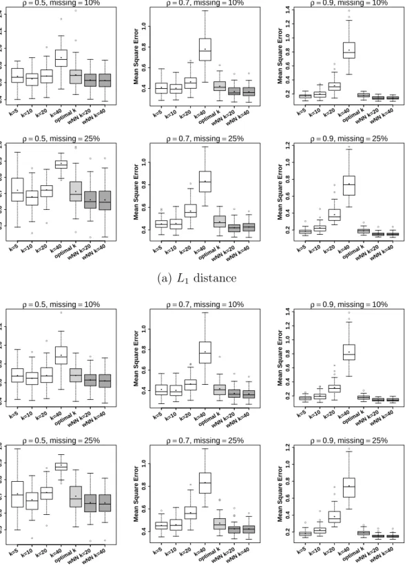
Fig. 2 shows the MSEs for the nearest neighbor imputation method with
fixed values of k = 5,10,20,40, for k chosen by cross-validation, and for the
weighted approach with k = 20,40 as the maximal neighbors. The boxplots of
MSE withL1 distance are shown in the upper panel of Fig. 2, andL2 distance
0 10 20 30 40 0.6 1.0 1.4 k MSE / MAE ● ● ● ● ● ● ● ●● ● ● ● ● ● ● ● ● ● ● ● ● ● ● ● ● ●● ● ● ● ● ●● ● ● ● ● ●● ● ● ● ● ● ● ● ● ● ● ●● ● ● ● ● ● ● ● ● ● ● ● ● ● ● ● ● ● ● ● ● ● ●● ● ● ● ● ● ● ρ =0.3, missing=5% 0 10 20 30 40 0.7 0.8 0.9 1.0 1.1 k MSE / MAE ● ● ● ●● ●●●● ● ● ● ● ● ●●●● ● ● ●● ● ●●●●● ●●●● ●● ● ●● ●● ● ● ● ● ●● ● ● ●● ● ●● ● ● ● ●● ● ●● ●● ● ● ● ●● ●● ● ●● ●● ● ● ●● ●● ρ =0.5, missing=5% 0 10 20 30 40 0.2 0.3 0.4 0.5 0.6 0.7 k MSE / MAE ● ● ● ● ● ● ●●●●●●●●● ●● ●● ● ●● ● ●● ● ● ● ● ● ● ● ● ● ● ● ● ● ● ● ● ● ●● ● ● ●● ●● ● ●● ●● ●●● ●● ●●●●●● ●● ●●● ● ●● ●● ● ● ● ● ρ =0.9, missing=5% 0 10 20 30 40 0.8 1.0 1.2 1.4 1.6 k MSE / MAE ● ● ● ● ● ● ● ●● ● ● ● ● ● ● ● ● ● ● ● ●● ● ●● ● ● ● ●● ●● ●● ● ● ●●●● ● ● ● ●●●● ● ● ● ● ● ● ● ● ● ● ● ● ● ● ● ● ● ● ● ● ●● ● ● ● ●● ● ● ● ● ● ● ρ =0.3, missing=25% 0 10 20 30 40 0.7 0.9 1.1 k MSE / MAE ● ● ● ● ● ●●● ● ● ● ● ●● ●● ●● ●● ●●●● ●●●● ●● ● ● ● ● ● ●● ●● ● ● ● ● ● ● ● ● ● ● ● ● ● ● ● ● ● ●● ● ●● ● ● ●● ●● ● ●●●● ●●●● ● ●● ● ρ =0.5, missing=25% 0 10 20 30 40 0.2 0.4 0.6 0.8 k MSE / MAE ● ●● ● ●● ●● ●●● ●●● ●● ●● ●● ● ● ● ● ● ● ● ● ● ● ● ● ● ●●● ●● ● ● ● ● ● ● ● ● ●● ●● ●● ●●●●●●●●● ●●● ●● ●● ●● ● ●● ● ●● ● ● ● ● ρ =0.9, missing=25%
Figure 1: Illustration of simulation study: Mean Squared Error (MSE) and Mean
Absolute error (MAE) for unweighted nearest neighbors using L2 metric for fixed
values of k (number of nearest neighbors), with 5% missing data (Upper panel) and 25% missing data (lower panel). Circles represent MSE and solid circles represent MAE.
are highly correlated. The MSE for ρ = 0.5, 10% missing, is larger than 0.6,
whereas for ρ = 0.9, 10% missing, it is below 0.2 (Fig. 2(a)). Similar results
are found for theL2 distance (Fig. 2(b)). Overall,L1 andL2 distances produce
nearly the same mean square errors in all the data settings.
In addition to the dependence on the correlation structure one objective of the simulation study is to investigate if cross-validation is able to find a proper
value fork, the number of nearest neighbors to be used. The boxplots show that,
although some specific values of kyield better performance, the procedure that
selectsk by cross-validation (denoted by optimalk) does fairly well. The other
point of interest is how the proposed weighted imputation performs. It is seen
that weighted imputation (wN N) always performs better than imputation for
fixed value of k, when the window width and the number of nearest neighbors,
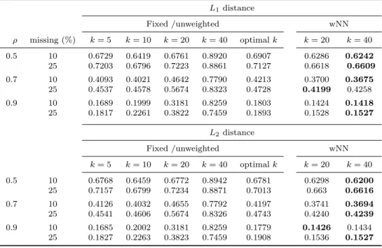
respectively, are chosen by cross-validation. The detailed results are shown in Table 1, where for each scenario the method that performed best is shown in boldface. It is seen that there is not much difference when allowing for 20 or 40 nearest neighbors in the weighting procedure. Nevertheless, for 40 the performance tends to be slightly better. In summary, weighted imputation turns out to be an attractive alternative that is computationally not more intensive
● ● ● ● 0.4 0.6 0.8 1.0 1.2 1.4
Mean Square Err
or ● ● ● ● ● ● ● ρ =0.5,missing=10% k=5 k=10 k=20 k=40 optimal kwNN k=20wNN k=40 ● ● ● ● 0.4 0.6 0.8 1.0
Mean Square Err
or ● ● ● ● ● ● ● ρ =0.7,missing=10% k=5 k=10 k=20 k=40 optimal kwNN k=20wNN k=40 ● ● ● ● ● 0.2 0.4 0.6 0.8 1.0 1.2 1.4
Mean Square Err
or ● ● ● ● ● ● ● ρ =0.9,missing=10% k=5 k=10 k=20 k=40 optimal kwNN k=20wNN k=40 ● ● ● ● ● ● ● ● ● ● 0.5 0.6 0.7 0.8 0.9 1.0
Mean Square Err
or ● ● ● ● ● ● ● ρ =0.5,missing=25% k=5 k=10 k=20 k=40 optimal kwNN k=20wNN k=40 ● ● ● ● ● 0.4 0.6 0.8 1.0
Mean Square Err
or ● ● ● ● ● ● ● ρ =0.7,missing=25% k=5 k=10 k=20 k=40 optimal kwNN k=20wNN k=40 ● ● ● ● ● ● ● ● ● 0.2 0.4 0.6 0.8 1.0 1.2
Mean Square Err
or ● ● ● ● ● ● ● ρ =0.9,missing=25% k=5 k=10 k=20 k=40 optimal kwNN k=20wNN k=40 (a) L1 distance ● ● ● ● 0.4 0.6 0.8 1.0 1.2
Mean Square Err
or ● ● ● ● ● ● ● ρ =0.5,missing=10% k=5 k=10 k=20 k=40 optimal kwNN k=20wNN k=40 ● ● ● ● ● 0.4 0.6 0.8 1.0
Mean Square Err
or ● ● ● ● ● ● ● ρ =0.7,missing=10% k=5 k=10 k=20 k=40 optimal kwNN k=20wNN k=40 ● ● ● ● ● ● ● ● ● 0.2 0.4 0.6 0.8 1.0 1.2 1.4
Mean Square Err
or ● ● ● ● ● ● ● ρ =0.9,missing=10% k=5 k=10 k=20 k=40 optimal kwNN k=20wNN k=40 ● ● ● ● ● ● ● 0.5 0.6 0.7 0.8 0.9 1.0
Mean Square Err
or ● ● ● ● ● ● ● ρ =0.5,missing=25% k=5 k=10 k=20 k=40 optimal kwNN k=20wNN k=40 ● ● ● ● ● ● ● ● 0.4 0.6 0.8 1.0
Mean Square Err
or ● ● ● ● ● ● ● ρ =0.7,missing=25% k=5 k=10 k=20 k=40 optimal kwNN k=20wNN k=40 ● ● ● ● ● ● ● ● ● ● ● 0.2 0.4 0.6 0.8 1.0 1.2
Mean Square Err
or ● ● ● ● ● ● ● ρ =0.9,missing=25% k=5 k=10 k=20 k=40 optimal kwNN k=20wNN k=40 (b) L2 distance
Figure 2: Boxplots of Mean Squared Error for NN Imputation using L1 distance
(a) and L2 distance (b). Imputation is done by using unweighted/fixed values of k
= 5, 10, 20, 40 nearest neighbors (white boxes), for optimal value of k selected by cross-validation (light grey boxes), and weighted approach (wN N) with maximum k
Table 1: MSE for NN imputation with weighted and unweighted approach using L1and L2distances L1distance Fixed /unweighted wNN ρ missing (%) k= 5 k= 10 k= 20 k= 40 optimalk k= 20 k= 40 0.5 10 0.6729 0.6419 0.6761 0.8920 0.6907 0.6286 0.6242 25 0.7203 0.6796 0.7223 0.8861 0.7127 0.6618 0.6609 0.7 10 0.4093 0.4021 0.4642 0.7790 0.4213 0.3700 0.3675 25 0.4537 0.4578 0.5674 0.8323 0.4728 0.4199 0.4258 0.9 10 0.1689 0.1999 0.3181 0.8259 0.1803 0.1424 0.1418 25 0.1817 0.2261 0.3822 0.7459 0.1893 0.1528 0.1527 L2distance Fixed /unweighted wNN k= 5 k= 10 k= 20 k= 40 optimalk k= 20 k= 40 0.5 10 0.6768 0.6459 0.6772 0.8942 0.6781 0.6298 0.6200 25 0.7157 0.6799 0.7234 0.8871 0.7013 0.663 0.6616 0.7 10 0.4126 0.4032 0.4655 0.7792 0.4197 0.3741 0.3694 25 0.4541 0.4606 0.5674 0.8326 0.4743 0.4240 0.4239 0.9 10 0.1685 0.2002 0.3181 0.8259 0.1779 0.1426 0.1434 25 0.1827 0.2263 0.3823 0.7459 0.1908 0.1536 0.1527
3 Weighted Neighbors Including Selection of Predictors
3.1 Selection of Dimensions
Traditionally the distances are computed from all the available components of the observations. However, as will be shown, in high-dimensional settings im-putation suffers from the curse of dimensionality. Therefore, we propose to compute distances from selected dimensions only. Since imputation is successful in particular when the predictors are highly correlated the selection of the di-mensions will be linked to the correlation between predictors. In the following an extended version of the weighted nearest neighbor imputation method is given that uses only the correlated predictors for the computation of the distances.
Let us consider imputation forxiin components(ois= 0). When computing
distances from the reduced data set{xj, ojs= 1}, we use an additional weight in
the distances. More concrete, forLq- distance one computes component-specific
distances by dq,C(xi,xj) ={ 1 mij p X l=1 |xil−xjl|I(ois = 1)I(ojs= 1)C(rsl)}1/q, (7)
whererslis the empirical correlation between covariatess, landC(.) is a convex
function defined on the interval [−1,1] that transforms the correlations into
weights. The transformation is constructed such that covariates that are strongly
correlated with componentsstrongly contribute to the computation of distances,
while components that are not correlated do not contribute to the distance.
One convex function C(.) that can be used is defined by
C(r) =
(
|r|
1−c−1−cc if |r|> c
It is linear in the absolute value of the correlation. If |rsj| ≤ c, the component
sdoes not contribute to the distance. Weights increase linearly with increasing
correlation and have weight 1 if |r| = 1. The threshold parameter c can be
chosen as fixed, for example, c = 0 or be considered as an additional tuning
parameter. A smoother function, which will also be used, is the power function
C(r) =|r|m, (9)
with m as additional tuning parameter. One problem is that rsl cannot be
computed since missing values are present in the data. Therefore we use a simple first step imputation by use of un-weighted five nearest neighbors and compute the correlations from the observed and imputed data. Then the actual imputation is carried out by using the correlations computed in the first step.
The weightedLqdistances with selection of dimensions includes the
calcula-tion of an addicalcula-tional tuning parameter. In addicalcula-tion to the tuning parameters for
the kernels,λ, one has to find an appropriate valuecfor the convex function (8)
or an integer m for the convex function (9). The parameters are chosen in the
same way asλin Section 2.3, namely by cross-validation. For the simultaneous
selection of the tuning parameters (λ,c) or (λ,m) cross-validation is computed
on on a two-dimensional grid of values. We will refer to this method as
wNNS-elect. We will characterize the linear function by c, and the power function by
the parameterm.
3.2 Evaluation of the Selected Weighted Neighbors
The simulation study in Section 2.5 showed that for highly correlated predictors
weighted nearest neighbors (wN N) perform better than unweighted distances.
Moreover, the results showed thatL1 andL2 distances have very similar
perfor-mance. In this section, the performance of the weighted approach with selection of predictors is investigated. We consider, in particular, two structures of the correlation matrix, blockwise correlation and autoregressive (AR) type correla-tion.
Blockwise Correlation Structure
Let the data matrixX(n×p), be partitioned intoX= [X(1),X(2),X(3)] such that
each element ofX(q) = [x
1,· · ·,xpq],q = 1, 2, 3, is a n×1 random vector. The
partitioned correlation matrix has the form
Σ = Σ11 ... Σ12 ... Σ13 · · · · Σ21 ... Σ22 ... Σ23 · · · · Σ31 ... Σ32 ... Σ33 ,
where Σii, is the matrix containing pairwise correlations ρ of the elements of
X(q), q = 1, 2, 3, that is, all components have (within) correlation (ρw). The
matrix Σij, contains the pairwise (between) correlations (ρb) between all the
AR-Type Correlation Structure
The second correlation structure we consider is the exponential orautoregressive
type correlation structure. An autoregressive of order 1 correlation matrix is
defined by
Σ = (ρ|i−j|),
wherei, j = 1, . . . , pand ρ is the pairwise correlation between predictors and p
is the number of predictors or variables in the data matrix.
Comparison of Fixed and Selected Values of Tuning Parameters
In the weighted imputation method considered in Section 2 (wN N), one tuning
parameterλfor the kernel weights had to be chosen. The method with selection
of predictors (7) involves one additional tuning parameter, c or m. In the
fol-lowing we first investigate if the data driven selection of the tuning parameters
(λ,c) or (λ,m) by cross-validation works.
We generated S = 50 samples of size n = 50 for p = 30 predictors drawn
from a multivariate normal distribution with N(0,ΣΣΣ). The correlation matrix
ΣΣΣ had either blockwise or autoregressive type structure. The data settings used
for the simulations were
Setting Structure Correlation missing 1 Blockwise ρw=0.7, ρb=0.1 10% 2 25% 3 ρw=0.9, ρb=0.1 10% 4 25% 5 Autoregressive ρ = 0.9 10% 6 25%
In the first type of ΣΣΣ, the predictors were chosen in three blocks of 10
pre-dictors each, that is, thep×1 random vectorX= [X(1),X(2),X(3)], is such that
X(1) = [X
1, . . . , X10], X(2) = [X11, . . . , X20],and X(3) = [X21, . . . , X30], where
each element of X(q), (q= 1,2,3) is a random variable. The variables within
each block were strongly correlated withρw = 0.70, 0.90, but nearly uncorrelated
with the variables in the other blocks with ρb = 0.10, for i, j = 1,2,3∀i6= j.
The second structure of ΣΣΣ considered is the autoregressive type of order 1 with
ρ = 0.9. In each sample, 10% and 25% of the total values were replaced by
missing values completely at random (MCAR).
In the simulation study, we used both convex functions (8) and (9) at fixed
levels and selected by cross-validation. For tuning parameter c in the linear
function (8) we consideredc∈ {0.2, 0.3, 0.4, 0.5}. Therefore, all the predictors
whose correlation with the sth predictors was less than or equal to specified
c, were discarded during the computation of distance. For the power function
(9), we used three values of the tuning parameter,m∈ {2,4,6}. The number of
nearest neighborskwas set to the maximum available neighbors. The large value
ofkwas chosen as the imputation procedure automatically chooses only relevant
neighbors for the calculation of the distance. For weighted NN imputation with
selection of predictors (wN N Select), cross-validation was used to compute MSE
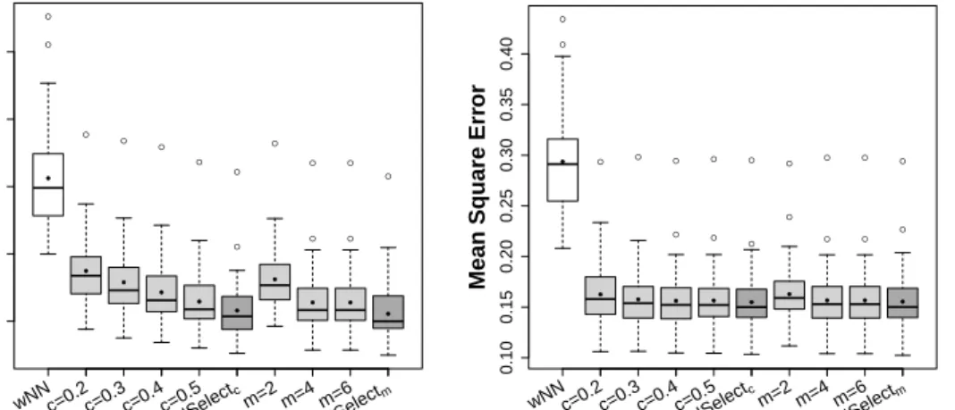
● ● ● ● ● ● ● ● ● ● ● ● ● ● 0.2 0.3 0.4 0.5 0.6
Mean Square Err
or ● ● ● ● ● ● ● ● ● ● AR(1), ρ =0.9,m=10% wNNc=0.2c=0.3c=0.4c=0.5 wNNSelect c m=2 m=4 m=6 wNNSelect m ● ● ● ● ● ● ● ● ● ● ● ● ● ● ● ● ● ● 0.10 0.15 0.20 0.25 0.30 0.35 0.40
Mean Square Err
or ● ● ● ● ● ● ● ● ● ● ρw=0.9, ρb=0.1,m=10% wNNc=0.2c=0.3c=0.4c=0.5 wNNSelect c m=2 m=4 m=6 wNNSelect m
Figure 3: Comparison of weighted imputation (white boxes), weighted with selection of predictors at fixed c= 0.2,0.3,0.4,0.5;m = 2,4,6 (light grey boxes) and with val-ues of tuning parameters chosen by cross-validation (wN N Selectc andwN N Selectm,
dark grey boxes) based on L2 distance in Autoregressive (left) and blockwise (right)
correlation structure. Solid circles within boxes show the mean values.
imputation without selection of predictors (wN N) the optimalλwas also chosen
on the basis of minimum MSE.
A visual comparison of weighted (wN N) and weighted with selection of
pre-dictors approaches for fixed and the selected values of tuning parameter of convex
functions c and m is given in Figure 3. Obviously, the method with selection
of predictors (wN N Select) performs much better than simple weighted NN
im-putation without selection of distances (wN N). Again the results from L1 and
L2 distances do not differ significantly. It is also seen that choice of tuning
pa-rameters cand m works well. For both type of correlation matrices it provides
smaller MSE than for fixed c and m. Similar results were obtained for other
simulation settings not shown here. Therefore we will proceed with the selected tuning parameter by double grid cross-validation.
Dependence on the Number of Predictors
Figure 3 already showed that the selection of sub spaces may yield better results. In the following we want to investigate how strong imputation based on distances computed from the whole set of predictors suffers when the number of predictors increases. Based on the results of the simulation study in the previous
sub-section we use cross-validation to select tuning parameters on a double grid (λ,
c) and (λ, m).
We use S=50 sample of size n = 50 with number of
predic-tors p ∈ {5,10,20,30,40,50,60,70,80,90,100} and n = 100 with p ∈
{5,10,20,30,40,50,60,70,80,90,100,120,150} from N(0,ΣΣΣ), where ΣΣΣ is the
AR(1) correlation matrix withρ= 0.9.
For comparison we use established nearest neighborhood methods that are
available in the R environment (R Core Team (2013)). The package impute
from Bioconductor uses nearest neighbors to impute the missing expression
val-ues of continuous variables (Hastie et al. (2013)). The functionkNNinRpackage
VIM(Templ et al. (2013)) deals with data consisting of continuous, count, binary
the computation of distances, but other metrics can also be used. Waljee et al. (2013) also used this package in their studies on clinical data. Another package
imputation(Wong (2013)) is available that imputes the missing data using the
algorithm provided by Troyanskaya et al. (2001). But the package sometimes does not yield estimates of all the missing data and such values are replaced by zeros by default.
Therefore, we chose the impute function from Bioconductor (Hastie et al.)
and the kNN function from package VIM (Templ et al. (2013)) as benchmarks
(shown as BIO and VIM respectively in Figure 5). Both methods use a
prede-fined or fixed number of nearest neighbors (k). To obtain comparable results we
selected the number of nearest neighbors (k) by using the same cross-validation
algorithm as discussed in Section 2.3. For weighted imputation without
selec-tion of variables, the tuning parameterλwas chosen using cross-validation with
m∗ corresponding to 10% and R = 10. The values of the tuning parameters
(λ, c) and (λ, m) were chosen via cross-validation on a double grid with m∗
corresponding to 10% and R = 10 for weighted imputation including selection
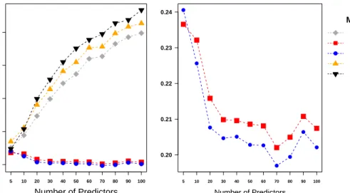
of predictors. 5 10 20 30 40 50 60 70 80 90 100 0.2 0.3 0.4 0.5 0.6 ● ● ● ● ● ● ● ● ● ● ● Number of Predictors
Mean Squared Error
5 10 20 30 40 50 60 70 80 90 100 0.20 0.21 0.22 0.23 0.24 ● ● ● ● ● ● ● ● ● ● ● Number of Predictors ● Methods wNN wNNSelectc wNNSelectm BIO VIM
Figure 4: Comparison of average MSEs at different number of predictors, n=50
(upper panel) and n= 100 (lower panel) using AR(1) correlation matrix withρ= 0.9 Fig. 4(left panel) shows the average MSEs for the imputation methods under consideration. It is seen that all imputation methods that use all the predictors show poor performance for increasing numbers of predictors. Although more information is available because more predictors are observed the performance deteriorates. In contrast, the methods that allow for selection of predictors can use the additional information. They perform better if the number of predictors increases. It also should be noted that with increasing number of predictors, the proposed weighting function (without selection) performs even better. Fig. 4(right panel) shows the performance of these methods in a separate panel. It is seen that, in particular, the convex function (9) yields good results in terms of mean squared errors even when the number of predictors is large.
Comparison of Weighted Imputation and Benchmarks
In the following we investigate more systematically the performance of the new
methods (wN N and wN N Select) and benchmark methods.
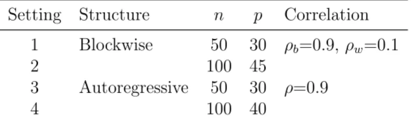
We consider S = 50 samples of size n = 50,100 from N(0,ΣΣΣ), where ΣΣΣ is
the correlation matrix of blockwise or autoregressive structure. The simulation settings are as follows:
Setting Structure n p Correlation 1 Blockwise 50 30 ρb=0.9, ρw=0.1
2 100 45
3 Autoregressive 50 30 ρ=0.9
4 100 40
For blockwise correlation with n = 50 (setting 1), in ΣΣΣ, the predictors
were chosen in three blocks of 10 predictors each, that is, the p × 1
ran-dom vector X = [X(1),X(2),X(3)], is such that X(1) = [X
1, . . . , X10], X(2) =
[X11, . . . , X20],and X(3) = [X21, . . . , X30], where each element of X(q), (q=
1,2,3) is a random variable. The variables within each block were strongly
correlated with ρw = 0.90, but nearly uncorrelated with the variables in
the other blocks with ρb = 0.10, for i, j = 1,2,3 ∀ i 6= j. Similarly, for
n = 100 (setting 2), the predictors were chosen in three blocks of 15
predic-tors each, that is, the p×1 random vector X = [X(1),X(2),X(3)], is such that
X(1) = [X1, . . . , X15], X(2) = [X16, . . . , X30],and X(3) = [X31, . . . , X45], where
each element of X(q), (q= 1,2,3) is a random variable. In setting 3 and 4, the
autoregressive type ΣΣΣ is of order 1 with ρ= 0.9.
The percentage of missing values in each data setting was set to
1%,5%,10%,20%,25% and 30% of the total values in design matrix completely
at random (MCAR). The tuning parameters for the proposed weighting function
wN N and wN N Select were chosen by cross-validation with m∗ = 10%. For
the benchmark methods, the number of nearest neighbors (k) was also chosen
by use of the same cross-validation algorithm.
Figure 5 compares the proposed weighted imputation methods with the ex-isting methods under Setting 1 and 3 at 5%, 15%, and 25% missing data. For the blockwise correlation structure (Fig. 5: upper panel for data setting 1),
the weighting functions using L2 metric with selection (shown as wN N Selectc
and wN N Selectm) and without selection of predictors (shown as wN N S)
pro-vides smaller MSE than the benchmarks (shown as BIO and VIM). The best
MSE is given by weighted selection of predictors (shown as wN N Selectc and
wN N Selectm). The convex functions (linear (8) and power (9)) used for the
se-lection of predictors provide nearly the same MSEs. For the autoregressive type correlation structure, (Fig. 5: lower panel for data Setting 3), at 5% missing the best MSE is obtained near 0.1, at 15% missing is near 0.2 and at 25% missing MSE is near 0.3. Therefore, in autoregressive type correlation the average MSE increases with an increase in the missing values. Similar results were obtained for Settings 2 and 4 with remaining missing percentages, see Table 2. In each data setting the value of smallest MSE is shown as boldfaced.
As seen from Table 2 for blockwise correlation withn= 50 (upper left panel),
at 1% missing data the smallest MSE was obtained by weighted selection of
predictors wN N Selectm, 0.1338. This value is much smaller than obtained by
● ● ● ● ● ●●● 0.2 0.6
Mean Square Err
or ● ● ● ● ● ρw=0.9, ρb=0.1,m=5% BIO VIM wNN wNNSelect c wNNSelect m ● ● ● 0.1 0.3 0.5
Mean Square Err
or ● ● ● ● ● ρw=0.9, ρb=0.1,m=15% BIO VIM wNN wNNSelect c wNNSelect m ● ● ● ● ● ● 0.2 0.4 0.6
Mean Square Err
or ● ● ● ● ● ρw=0.9, ρb=0.1,m=25% BIO VIM wNN wNNSelect c wNNSelect m ● ● ● ● 0.2 0.6 1.0
Mean Square Err
or ● ● ● ● ● AR(1), 5% missing BIO VIM wNN wNNSelect c wNNSelect m ● ● ● 0.2 0.4 0.6
Mean Square Err
or ● ● ● ● ● AR(1), 15% missing BIO VIM wNN wNNSelect c wNNSelect m ● ● ● ● ● ● ● ● ● 0.3 0.5 0.7
Mean Square Err
or ● ● ● ● ● AR(1), 25% missing BIO VIM wNN wNNSelect c wNNSelect m
Figure 5: Comparison of wN N Select (dark grey boxes), wN N (light grey boxes)
imputation using L2 metric, and two benchmarks (white boxes); impute from
Bio-conductor (shown as BIO) &VIM (shown as VIM) using Blockwise (upper panel) and Autoregressive (lower panel) correlation structure
obvious that the selection of dimension (wN N Select) reduces the MSEs when
only the relevant information from selected predictors is used. Similar results are
obtained forn= 100 (Table 2: lower left panel). For the blockwise structure with
1% to 20% missing data there is not much difference concerning the alternative convex function used in the weighting procedure. But when percentage of the missing data is greater than 20% of the data matrix, the weighted function (wN N Delectm) with the power function (9) shows the best MSEs irrespective
of the correlation structure.
In the case of autoregressive correlation with n = 50 (Table 2: upper
right panel), weighted selection of predictors with convex function (9), namely
wV V Selectm, usingL2 metric provides smaller MSE (e.g., 0.1580 for 1%
miss-ing values and 0.3416 for 30% missmiss-ing). Both of these values are much smaller
than obtained by wN N and benchmark imputation methods. Moreover, the
best MSE is obtained by weighted L2 with selection of predictors using convex
function (9), namelywN N Selectm. Similar results are found forn= 100 (Table
2: lower right panel).
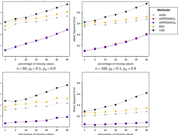
A comparative view of the performance for different levels of missing per-centages for blockwise (lower panel) and autoressive (upper panel) is shown in Figure 6. To make them comparable all the plots are drawn on the same scale. It is seen that the mean squared errors get larger with increasing percentage of missing values. But the curve is more flatter when the data is from blockwise correlation. Overall, the proposed weighting functions distinctly outperform the
available methods in all the data settings, in particular the wN N Selectc and
T able 2: Comparison of MSE for w eigh ted L2 NN imputation with b enc hmarks Blo ckwise Correlation AR(1) Correlation w eig hted Benc hmark w eig hted Benc hmark n missing w N N w N N S el ect c w N N S el ect m B I O V I M w N N w N N S el ect c w N N S el ect m B I O V I M 50 1% 0.2566 0.1352 0.1338 0.2846 0.3385 0.3436 0.1596 0.1580 0.3765 0.4133 5% 0.2642 0.1457 0.1457 0.3057 0.3350 0.3952 0.1911 0.1859 0.4288 0.4420 10% 0.2722 0.1488 0.1492 0.3103 0.3530 0.4125 0.2200 0.2143 0.4382 0.4532 15% 0.2903 0.1555 0.1547 0.3286 0.3860 0.4166 0.2461 0.2422 0.4468 0.4854 20% 0.2888 0.1615 0.1605 0.3284 0.4189 0.4304 0.2745 0.2688 0.4662 0.5118 25% 0.3204 0.1853 0.1842 0.3640 0.4549 0.4517 0.3075 0.3054 0.4841 0.5430 30% 0.3170 0.1930 0.1930 0.3592 0.4807 0.4667 0.3461 0.3416 0.5055 0.5735 100 1% 0.2044 0.1271 0.1272 0.2325 0.2438 0.3720 0.1534 0.1503 0.3886 0.4126 5% 0.2062 0.1209 0.1212 0.2301 0.2586 0.3896 0.1727 0.1674 0.4105 0.4263 10% 0.2140 0.1260 0.1262 0.2400 0.2846 0.3870 0.1894 0.1839 0.4089 0.4584 15% 0.2184 0.1303 0.1304 0.2463 0.3031 0.4013 0.2130 0.2086 0.4221 0.4802 20% 0.2249 0.1337 0.1339 0.2522 0.3403 0.4126 0.2362 0.2318 0.4363 0.5074 25% 0.2343 0.1377 0.1376 0.2651 0.3762 0.4251 0.2667 0.2621 0.4490 0.5440 30% 0.2409 0.1434 0.1433 0.2725 0.4100 0.4385 0.3034 0.2995 0.4634 0.5791
1 5 10 15 20 25 30 0.2 0.3 0.4 0.5 ● ● ● ● ● ● ● AR(1),n=50, ρ =0.9
percentage of missing values
Mean Squared Error
1 5 10 15 20 25 30 0.2 0.3 0.4 0.5 ● ● ● ● ● ● ● AR(1),n=100, ρ =0.9
percentage of missing values
Mean Squared Error
1 5 10 15 20 25 30 0.2 0.3 0.4 0.5 ● ● ● ● ● ● ● n=50, ρb=0.1, ρw=0.9
percentage of missing values
Mean Squared Error
1 5 10 15 20 25 30 0.2 0.3 0.4 0.5 ● ● ● ● ● ● ● n=100, ρb=0.1, ρw=0.9
percentage of missing values
Mean Squared Error
● Methods wNN wNNSelectc wNNSelectm BIO VIM
Figure 6: Comparison of wN N Select at different percentages of missing data in
autoregressive (upper panel) and blockwise (lower panel) structure. The tuning pa-rameters (λ, c) and (λ, m) selected by cross-validation.
4 Case Studies
In this section we use several real data sets to compare imputation methods. We use two data sets from genetics and two data sets from non-genetic studies. The complete data sets without any missing values were used so that we can compare the results.
4.1 Gene Expression Data
In particular, gene expression data often contain missing values. Some previous studies on imputation of missing values in gene expression data are by Brock et al. (2008), Wasito and Mirkin (2005), Troyanskaya et al. (2003), Nguyen et al. (2004), Hastie et al. (1999), and Dudoit et al. (2002). We used subsets of gene expression data on two different types of human tumor namely lym-phomas and leukemia. These data sets can be downloaded from the website http://www.gems-system.org/.
The data sets were preprocessed before using for imputation. A significance
analysis was carried out to identify differentially expressed genes using samr
package in R (R Core Team (2013)). The selected genes were standardized to
DLBCL Data
The gene expression data on Lymphomas was collected from 77 patients on
6,817 genes. The response was Diffuse large B-cell lymphomas (DLBCL) with
n=58 patients or follicular lymphomas (FL) with n=19 patients. We used in
our analysis the first 100 significant genes (variables) and all 77 patients.
Leukemia Data
The second data we use is based on three types of leukemia; Acute myeloge-nous leukemia (AML), acute lympboblastic leukemia (ALL) B-cell, and ALL T-cell. The complete data consists of the gene expression on 5,328 variables of 72 patients. The data for all 72 patients for first 100 significant genes was used.
4.2 Non-Gene Expression Data
LSVT Voice Rehabilitation Data Set
The LVST (Lee Silverman Voice Treatment) Global, a company specialising in voice rehabilitation assists the people with Parkinson’s disease (PD). The data set was originally collected to determine the most parsimonious feature subset which helps to predict the binary response. The data are composed of a range of biomedical speech signal processing algorithms from 14 people who have been diagnosed with Parkinson’s disease undergoing LSVT. The original study used 310 algorithms (predictors) to characterize 126 speech signals (samples). The response variable is binary, acceptable vs unacceptable phonation during rehabilitation. More information on data can be found in Tsanas et al. (2013). The data can be downloaded from the UCI Machine Learning Repository.
LIBRAS Movement Database
The data set contains 15 classes of 24 instances each, where each class references to a hand movement type in LIBRAS. The hand movement is represented as a bidimensional curve performed by the hand in a period of time. The curves were obtained from videos of hand movements, with the Libras performance from 4 different people, during 2 sessions. Each video corresponds to only one hand movement and has about 7 seconds. The total data consists of 360 instances of 90 numeric attributes. More information on data can be found in Dias et al. (2009). The data set is available on the UCI Machine Learning Repository.
All the variables were standardized before processing. The NN imputation techniques were applied to these four data sets by artificially setting 5% of the observations as missing completely at random (MCAR). The missing values were imputed by using weighted nearest neighbors with selection of variables (wN N Select) with the tuning parameters chosen by cross-validation. Also for the benchmark methods, the number of nearest neighbors was selected by cross-validation. The procedure was repeated 10 times for all methods. The resulting averaged MSEs are shown in Table 3. The smallest MSE for each data set is shown in boldface.
In all these case studies, the minimum value of average MSE was obtained
by one of the new imputation methods. For DLBCL data, the minimum,
0.5993, was obtained for the L1 metric with the convex function (9) shown
as wN N Selectm. The the impute function in Bioconductor package gave the
Table 3: Average MSE results from real data sets
L1 metric L2 metric Benchmark
DATA wN N Selectc wN N Selectm wN N Selectc wN N Selectm BIO VIM
DLBCL 0.6424 0.5993 0.6504 0.6078 0.7267 0.7889
Leukemia 0.7620 0.7461 0.7620 0.7292 0.8709 0.8272
LVST 0.4401 0.4427 0.4142 0.4087 0.5821 0.5731
LIBRAS 0.0799 0.0752 0.0353 0.0350 0.2903 0.3964
Similar results are found for the leukemia data with 0.7279 as minimal average
MSE from wN N Selectm using L2 metric. For LVST and LIBRAS movement
data sets, the smallest MSE is obtained fromwN N Selectm using L2 metric. It
is obvious from table 3 that the proposed imputation procedure yields better
results than the Bioconductor and the VIMpackages in all the data sets.
5 Concluding Remarks
The main objective of this study was to introduce an improved nearest neighbor procedure for the imputation of missing values. The simulation results show that
the proposedweighted imputation estimate performs better than the fixed or the
un-weighted approach. We also compared L1 and L2 metrics in the weighted
imputation of missing data and found L2 metric to be slightly better than L1
metric. The use of kernel functions for the computation of weights decreases the imputation error. Simulation results (not presented here) suggest that the Gaussian kernel provides smaller MSEs than other kernel functions.
To cope with the problem of high dimensional data, we proposed an im-putation method with a weighted selection of predictors. The procedure uses cross-validation for optimal selection of the tuning parameters. In particular, for highly correlated data, the proposed NN imputation procedure shows promising results, also in the case of a high proportion of missing data. The simulation studies as well as real data sets confirm these results.
References
Allison, P. D. (2001). Missing data. Number 136. Sage.
Atkeson, C., A. Moore, and S. Schaal (1997). Locally weighted learning.
Artifi-cial Intelligence Review 11(1-5), 11–73.
Batista, G. E. and M. C. Monard (2002). A study of k-nearest neighbour as an
imputation method. HIS 87, 251–260.
Bø, T. H., B. Dysvik, and I. Jonassen (2004). Lsimpute: accurate estimation of
missing values in microarray data with least squares methods. Nucleic Acids
Research 32(3), e34–e34.
Brock, G. N., J. R. Shaffer, R. E. Blakesley, M. J. Lotz, and G. C. Tseng (2008). Which missing value imputation method to use in expression profiles:
a comparative study and two selection schemes. BMC Bioinformatics 9(1),
Cai, Z., M. Heydari, and G. Lin (2006). Iterated local least squares
microar-ray missing value imputation. Journal of Bioinformatics and Computational
Biology 4(05), 935–957.
Dias, D. B., R. C. Madeo, T. Rocha, H. H. Biscaro, and S. M. Peres (2009). Hand movement recognition for brazilian sign language: a study using
distance-based neural networks. InNeural Networks, 2009. IJCNN 2009. International
Joint Conference on, pp. 697–704. IEEE.
Dudoit, S., J. Fridlyand, and T. P. Speed (2002). Comparison of discrimination
methods for the classification of tumors using gene expression data. Journal
of the American Statistical Association 97, 77–87.
Eskelson, B. N., H. Temesgen, V. Lemay, T. M. Barrett, N. L. Crookston, and A. T. Hudak (2009). The roles of nearest neighbor methods in imputing
missing data in forest inventory and monitoring databases. Scandinavian
Journal of Forest Research 24(3), 235–246.
Feten, G., T. Almoy, and A. H. Aastveit (2005). Prediction of missing values
in microarray and use of mixed models to evaluate the predictors. Statistical
Applications in Genetics and Molecular Biology 4(1), 10.
Fix, E. and J. L. Hodges (1951). Discriminatory analysis-nonparametric dis-crimination: consistency properties. Technical report, DTIC Document. Gower, J. C. (1971). A general coefficient of similarity and some of its properties.
Biometrics, 857–871.
Hastie, T., R. Tibshirani, B. Narasimhan, and G. Chu (2013). impute: impute:
Imputation for microarray data.http://www.bioconductor.org/packages/
release/bioc/html/impute.html. R package version 1.36.0.
Hastie, T., R. Tibshirani, G. Sherlock, M. Eisen, P. Brown, and D. Botstein (1999). Imputing missing data for gene expression arrays.
Hron, K., M. Templ, and P. Filzmoser (2010). Imputation of missing values
for compositional data using classical and robust methods. Computational
Statistics and Data Analysis 54(12), 3095–3107.
Hudak, A. T., N. L. Crookston, J. S. Evans, D. E. Hall, and M. J. Falkowski (2008). Nearest neighbor imputation of species-level, plot-scale forest
struc-ture attributes from lidar data. Remote Sensing of Environment 112(5),
2232–2245.
Johansson, P. and J. Hakkinen (2006). Improving missing value imputation of
microarray data by using spot quality weights. BMC Bioinformatics 7(1),
306.
Junninen, H., H. Niska, K. Tuppurainen, J. Ruuskanen, and M. Kolehmainen (2004). Methods for imputation of missing values in air quality data sets.
Atmospheric Environment 38(18), 2895–2907.
Kim, H., G. H. Golub, and H. Park (2005). Missing value estimation for dna
microarray gene expression data: local least squares imputation.
Kim, K.-Y., B.-J. Kim, and G.-S. Yi (2004). Reuse of imputed data in microarray
analysis increases imputation efficiency. BMC Bioinformatics 5(1), 160.
Liew, A. W.-C., N.-F. Law, and H. Yan (2011). Missing value imputation for gene expression data: computational techniques to recover missing data from
available information. Briefings in Bioinformatics 12(5), 498–513.
Little, R. J. and D. B. Rubin (1987). Statistical analysis with missing data,
Volume 539. Wiley New York.
Malarvizhi, M. R. and D. A. S. Thanamani (2012). K-nearest neighbor in missing
data imputation. International Journal of Engineering Research and
Devel-opment 5.
Moorthy, K., M. Saberi Mohamad, and S. Deris (2014). A review on missing
value imputation algorithms for microarray gene expression data. Current
Bioinformatics 9(1), 18–22.
Myrtveit, I., E. Stensrud, and U. H. Olsson (2001). Analyzing data sets with missing data: an empirical evaluation of imputation methods and
likelihood-based methods. Software Engineering, IEEE Transactions on 27(11), 999–
1013.
Nguyen, D. V., N. Wang, and R. J. Carroll (2004). Evaluation of missing value
estimation for microarray data. Journal of Data Science 2(4), 347–370.
Ouyang, M., W. J. Welsh, and P. Georgopoulos (2004). Gaussian mixture
clus-tering and imputation of microarray data. Bioinformatics 20(6), 917–923.
R Core Team (2013). R: A language and environment for statistical computing.
http://www.R-project.org/.
Schafer, J. L. (2010). Analysis of incomplete multivariate data. CRC press.
Scheel, I., M. Aldrin, I. K. Glad, R. S ˜A¸rum, H. Lyng, and A. Frigessi (2005).
The influence of missing value imputation on detection of differentially
ex-pressed genes from microarray data. Bioinformatics 21(23), 4272–4279.
Sehgal, M. S. B., I. Gondal, and L. S. Dooley (2005). Collateral missing value imputation: a new robust missing value estimation algorithm for microarray
data. Bioinformatics 21(10), 2417–2423.
Templ, M., A. Alfons, A. Kowarik, and B. Prantner (2013). Vim: Visualization
and imputation of missing values. http://CRAN.R-project.org/package=
VIM. R package version 4.0.0.
Troyanskaya, O., D. Botstein, and R. Altman (2003). Missing value estimation.
In D. Berrar, W. Dubitzky, and M. Granzow (Eds.),A Practical Approach to
Microarray Data Analysis, pp. 65–75. Springer US.
Troyanskaya, O., M. Cantor, G. Sherlock, P. Brown, T. Hastie, R. Tibshirani, D. Botstein, and R. B. Altman (2001). Missing value estimation methods for
dna microarrays. Bioinformatics 17(6), 520–525.
Tsanas, A., M. A. Little, C. Fox, and L. O. Ramig (2013). Objective automatic assessment of rehabilitative speech treatment in parkinson’s disease.
Waljee, A. K., A. Mukherjee, A. G. Singal, Y. Zhang, J. Warren, U. Balis, J. Marrero, J. Zhu, and P. D. Higgins (2013). Comparison of imputation
methods for missing laboratory data in medicine. BMJ Open 3(8).
Wasito, I. and B. Mirkin (2005). Nearest neighbour approach in the least-squares
data imputation algorithms. Information Sciences 169(1), 1–25.
Wong, J. (2013). imputation: imputation. http://CRAN.R-project.org/
package=imputation. R package version 2.0.1.
Yoon, D., E.-K. Lee, and T. Park (2007). Robust imputation method for missing
values in microarray data. BMC Bioinformatics 8(Suppl 2), S6.
Zhang, X., X. Song, H. Wang, and H. Zhang (2008). Sequential local least
squares imputation estimating missing value of microarray data. Computers