DISTRIBUTION STATEMENT A: Approved for public release; distribution is unlimited.
This project was funded by the National Aeronautics and Space Administration (NASA) Marshall Space Flight Center (MSFC) under Jacobs ESTS Contract NNM05AB50C, Task Order 33-000002-CU.
VALIDATION AND SIMULATION OF ARES I SCALE MODEL ACOUSTIC TEST - 1 - PATHFINDER DEVELOPMENT
G. C. Putnam
NASA / Marshall Space Flight Center / ER42 / All Points Logistics Huntsville, AL
ABSTRACT
The Ares I Scale Model Acoustics Test (ASMAT) is a series of live-fire tests of scaled rocket motors meant to simulate the conditions of the Ares I launch configuration. These tests have provided a well documented set of high fidelity measurements useful for validation including data taken over a range of test conditions and containing phenomena like Ignition Over-Pressure and water suppression of acoustics. To take advantage of this data, a digital representation of the ASMAT test setup has been constructed and test firings of the motor have been simulated using the Loci/CHEM computational fluid dynamics software. Within this first of a series of papers, results from ASMAT simulations with the rocket in a held down configuration and without water suppression have then been compared to acoustic data collected from similar live-fire tests to assess the accuracy of the simulations. Detailed evaluations of the mesh features, mesh length scales relative to acoustic signals, Courant-Friedrichs-Lewy numbers, and spatial residual sources have been performed to support this assessment. Results of acoustic comparisons have shown good correlation with the amplitude and temporal shape of pressure features and
reasonable spectral accuracy up to approximately 1000 Hz. Major plume and acoustic features have been well captured including the plume shock structure, the igniter pulse transient, and the ignition overpressure. Finally, acoustic propagation patterns illustrated a previously unconsidered issue of tower placement inline with the high intensity overpressure propagation path.
INTRODUCTION
The Ares I Scale Model Acoustics Test (ASMAT) was a series of live-fire tests of a scaled rocket motor meant to simulate the conditions of the Ares I launch configuration. [1] Its primary goals were the validation of the acoustic environments for the vehicle and the predicted acoustic loads. As secondary goals, it also enabled validation of analytical and computational models. In particular, the ASMAT tests provided a well documented set of high fidelity measurements that were useful for validation of Computational Fluid Dynamics (CFD) prediction abilities. These measurements were taken over a range of test conditions and were used to validate CFD prediction of phenomena like Ignition Over-Pressure (IOP) and water suppression of the liftoff environment.
To take advantage of this data and meet the computational validation goal, it was necessary to build a digital representation of the ASMAT test setup and then simulate the test firings using Computational Fluid Dynamics (CFD) software. This paper will describe the construction and execution of the initial ASMAT simulations, deemed the Pathfinder study, using the Loci/CHEM software package. Further papers have then been written to discuss the specific simulations and effects of rocket elevation, launch mount configuration changes, and water deluge inclusion.
DESCRIPTION OF THE LOCI/CHEM SOFTWARE
Loci/CHEM is a density-based finite-volume CFD program built upon the Loci framework. [2; 3; 4; 5; 6; 7]
Loci is a framework that performs the coordination and interaction of a collection of numerical kernels and methods. This collection of numerical kernels and methods support the different capabilities in the Loci/CHEM program. Among the current capabilities in the Loci/CHEM program are: support for arbitrary meshes, several different time integration schemes, and
variable time step (i.e., fixed CFL) for steady-state calculations, different turbulent models such as Menter’s baseline and Menter’s Shear Stress Transport (SST) model, pre-conditioning for low Mach number flows, finite-rate chemistry, and conjugate heat transfer. Also, through the Loci framework, Loci-CHEM supports the use of distributed memory computers for parallel computing. A detailed documentation of the equation formulation and numerical approaches may be found in the Loci/CHEM Users manual.
Loci/CHEM has two second-order accuracy temporal methods of advancing the CFD simulation in time. Both methods use a second-order, three-point, backward scheme. The baseline time-advancement method is selected by setting the time_integration parameter to second_order within the variable input file. An additional time advancement method which limits the time step only in the residual Jacobian used to advance the solution to the next Newton iteration, is activated by setting the time_integration parameter to time_accurate within the variable input file. In this mode, the Jacobian time step for any given cell is chosen such that it is the smallest of the following two values: 1) the user-specified maximum time-step value dtmax, and 2) the time step required to produce no more than an estimated urelax percent change in temperature, pressure, or density. This decreased time step in the Jacobian calculation may slow the speed at which the solution advances per Newton iteration within the timestep. It is this slowing of development which can potentially increase the robustness of an unsteady simulation. When using the time_accurate method, the user should confirm adequate residual drop as a function of Newton iterations, adding more Newton iterations if necessary to overcome the potentially slower convergence of the Newton iteration.
SIMULATION MODEL
The model of the ASMAT setup used for CFD simulations was constructed starting from a Computer Aided Design (CAD) model of the test. This model was converted into IGES format and imported into the ANSA geometry pre-processing tool. ANSA was used to mesh the simulation region over its surface, and export the result as a NASTRAN surface mesh. [8] This surface was then imported into the SimCenter suite of tools, where it was first checked for quality using the SolidMesh software and then used to generate a binary double UGRID format
volumetric mesh with the AFLR3 software. [9] Finally, this file was converted to the native VOG volumetric mesh format for Loci/CHEM using the “ugrid2vog” utility in Loci/CHEM’s tools, and checked once more for quality with the “vogcheck” utility.
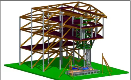
The CAD model of the ASMAT test was a highly detailed design model meant for the construction of the test setup, and included not only the bulk details of the rocket and pad, but also the water systems, fasteners, cabling, support structure, and surrounding environment. A rendering of this full model can be seen in Figure 1. As the full model was overly detailed for the purposes of this simulation, only the immediate structures of the rocket, pad, tower, and water systems were retained, and most small items like fasteners were removed.
After the CAD files had been transferred to ANSA, they were verified against imagery, cleaned, defeatured, and merged into a water-tight simulation volume. Defeaturing, as well as later surface meshing, was approached with four priorities in mind: 1) Fidelity in the path of the plume, 2) Fidelity near the source of acoustic waves, 3) Fidelity in the vicinity of sensors of interest, and 4) Fidelity over the path of acoustic waves. A selection of roughly 20 sensors was known at the time of model creation, and these locations drove much of the modeling process.
Figure 1 - Full CAD Model for ASMAT Test Setup
The result of this approach was that the highest resolution regions were the rocket nozzle and the upper section of the launch mount, as they were in the plume path and near the source of acoustic waves. All nozzles, water inlet slots, and acoustic plates were retained within the launch mount plume hole, and the main deflector and mushroom caps also remained largely unchanged by defeaturing, as they all came under direct plume impingement.
To encapsulate the platform in a water tight region, the ground plane of the test stand was extended into a surface which ran two pad lengths in the direction of both plume holes, and one pad width to either side of the stand. This was then placed in a box, which rose straight up from the edges of the surface to a height that was roughly 1.5 times as tall as the test stand. The final dimensions of this box were 1358” x 464” x 417”. A rendering of this simulation enclosure can be seen below in Figure 2. This entire region was then surface meshed using ANSA.
Figure 2 - ASMAT Simulation Bounds
Upon completion of the surface meshing operation, and successful creation of a computational domain with limited high aspect ratio surface cells, the surface mesh was transferred to the AFLR3 software using the NASTRAN format so that a volume mesh could be created. For the Pathfinder simulations, AFLR3 version 13.0.5 for x86_64 bit Linux was used to create both meshes. For the first mesh, the final volume contained 22.6 million nodes and 50.2 million cells, with the vast majority of these cells being prisms (84% of all cells). For the second mesh, all of those numbers nearly doubled, with 41 million nodes, 101 million cells. The ratio of tetrahedrons to prisms went down slightly, with only 71% of the cells being prisms.
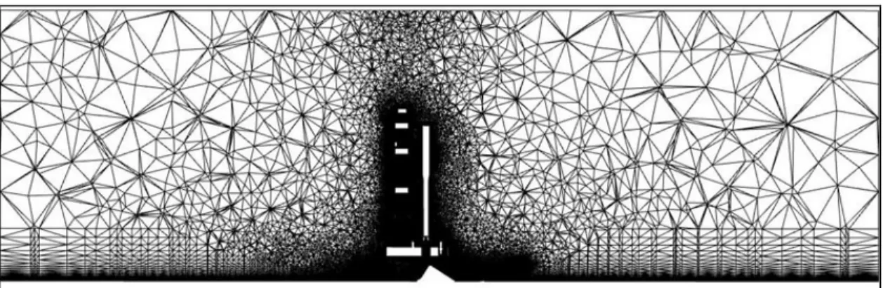
In Figure 3 below, the overall nature of the meshed regions can be seen with a cutting plane through the centerline of the rocket and mesh. The cut shown is for the second mesh, but
at this distance from the test stand, the mesh quickly dropped to a very low resolution and the changes which were made to the plume path and tower cells for the second mesh were only barely visible as an increase in density at the top of the tower and the ends of the trenches.
Figure 3 - Section of Volume Mesh through Vehicle and Flame Trench
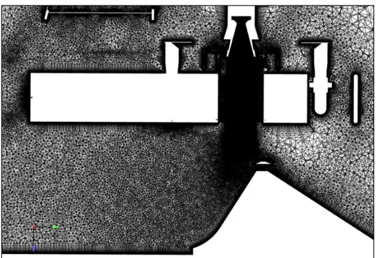
Within Figure 4 and Figure 5, a second view of the centerline is shown, but focused on the critical areas within the plume core, below the deck, and just above the deck surface. In the trench, there was an order of magnitude difference in cell size between the upper and lower surfaces of the trench. For the first mesh, the plume source was also only incorporated for portions of its length, with an obvious lack of cell resolution apparent near the exit of the plume hole. This may have been an issue in volume generation where AFLR3 was forced to make a trade between nearby wall boundary layer resolution and the desired source resolution. For the second mesh, both these issues were repaired, with a high density column present for the plume path up to the point of impact with the deflector, and a smooth cell size throughout the trench.
Figure 5 - Section of Volume Mesh in Vicinity of Active Trench – Refined Mesh
Shifting to the above deck features, the tower showed a relatively uniform cell density throughout its volume, with sharp increases present near the boundary layers of each beam. While the overall density for the first mesh was high compared to the farfield size, or even the density near the roof of the trench, it was still an order of magnitude less dense than the cells in the vicinity of the rocket plume. In addition, for many beams, the cell density was insufficient to ensure three cells spanning each beam. This created issues for the CFD program’s ability to resolve the presence of the beam in space. For the second mesh, this issue was fixed with an approximately uniform doubling of mesh density near all of the beams. Also of note was the somewhat low resolution area between the surface of the launch pad and the first floor of the tower. This was not changed during the improvements for the second mesh, as it was not near any microphones of note, but should be improved for later runs to resolve reflections at elevation. MESH COURANT-FRIEDRICHS-LEWY NUMBER
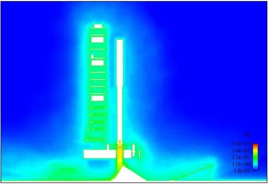
In addition to visualization of the CFD mesh scaling and distribution, the Courant-Friedrichs-Lewy (CFL) conditions were also plotted for the mesh after a solution was computed. In Figure 6 the CFL numbers for the ASMAT simulation have been plotted at the point of
completion. The simulation has reached a quasi-steady state at the point of plotting, with the plume fully established and only limited transient behavior observed near the trench exit.
From this image, it can be seen that there are three major regions of low resolution cells which could limit simulation resolution. These are the previously noted section of low resolution cells below the deck, the band of cells wrapping around the end of the launch pad near the trench exit, and the sheath of lower resolution cells which wraps the top of the vehicle. Low resolution in this context means that the cells display a CFL number of < 1. The two groups of cells near the trench are particularly important, as they would directly affect results for IOP trench waves diffracting around the end of the launch platform.
Figure 6 - Section of Mesh Showing CFL Conditions for Launchpad
In general, it appears that the meshing strategy described earlier was largely successful, with most near vehicle regions exhibiting CFL numbers of 1-10, near plume regions exhibiting values from 10-100, and internal plume features exhibiting values from 100-1000. A noteworthy region of lower resolution within the plume features is the boundary layer within the nozzle chamber, which displays bands of CFL dropping to 50 or less. Meanwhile, the highly refined plume source cylinder displays markedly higher CFL numbers than any other region of the simulation, with CFL values on the surface of the cylinder reaching > 1000.
PLUME MODELLING
For the ASMAT simulations, only a very limited set of data was available for the RATO motor performance. No axisymmetric flow solution was available for the motor, and even the mass flow rate was only defined for the maximum steady state condition. The only information available for the RATO performance was the chamber pressure rise rate, which had been determined from a series of case mounted strain gage measurements and head end chamber pressure measurements during horizontal tests. As such, it was judged that the best
methodology for the ASMAT simulations would be to use a source condition located within the nozzle chamber. This source would represent upstream effluent entering the nozzle chamber and would have a profile determined from the chamber pressure history.
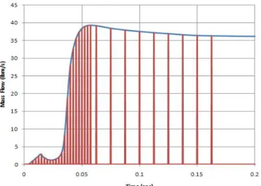
The burning composition of the RATO exhaust was unknown, and an approximation was made to use the heavy gas models, [10] which had been developed for Shuttle SRB simulations, and reduce the plume flowfield chemistry model from a multiple species mixing approach to the mixing of only a composite, pseudo-species. This was considered reasonable, as the chemical composition of the ASMAT fuel was similar to the Shuttle SRBs. The mass flow rate profile for the pseudo-species was estimated using techniques similar to the initial Shuttle modeling approach. Given the known pressure history of the chamber and the steady state flow rate, the time behavior of pressure was used as the basis for mass flow by sampling the pressure values, and then scaling them so that the final flow rate matched the steady state mass flow.
In its traditional implementation, this technique is known to be imprecise, due to a dependence on only the chamber pressure at the head end of the rocket. However, for the ASMAT tests, further data sets from strain gages mounted around the perimeter of the rocket
were also available, which increased the fidelity of the source pressure trace, and the resulting mass flow curve. [11] The final curve for the mass flow rate in the nozzle chamber can be seen in Figure 7. Samples were taken every 2.5 ms prior to 0.06 seconds and every 12.5 ms after.
Figure 7 - Calculated ASMAT Mass Flow Profile IGNITION TRANSIENT
Between the initial and refined simulations, a change was made to the profile of the ignition transient profile over the first ~25 ms of the simulation. In the initial simulations, it was noted that a direct translation of chamber pressure to mass flow produced flow rates which rose too gradually, resulting in spurious pressure oscillations at sensors prior to their real-world timing and a lack of a sharp transient at motor start. It was thought that this lack was due to the absence of a throat plug expulsion being modeled. In the real test article, a foam plug was set into the nozzle and blocked the flow until a certain pressure state was reached, which broke the foam and then expelled it in a sharp event.
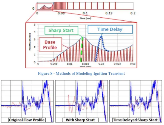
Two methods were tested in short simulations to try and mimic this behavior prior to starting the refined simulation. The first method was to produce a sharp start of mass flow at the point of maximum pressure during the ignition transient, as it was reasoned that the drop in pressure from ~15 ms to ~30 ms was due to flow after the throat plug breakage. This method, shown as the Sharp Start line in the zoomed in portion of Figure 8 below, reproduced the sharp transient effects at motor start, but resulted in flow, and transmitted signals, too early in the simulation. To correct for this mismatch, a time delay of ~5 ms for the start of mass flow was implemented, which resulted in the main mass flow peak shifting to ~20 ms after simulation start, and can be seen as the Time Delay line in Figure 8.
The Time Delay method with a sharp start reproduced the pressure behavior of the startup transient extremely well. It matching not only the pressure spike at start over multiple sensors, but also the trailing oscillations for several milliseconds. The resulting pressure signals transmitted with the three methods to a sensor near the nozzle (IOP_MO3) can be seen below in Figure 9. Based on these results, the second, delayed method of modeling the startup transient was used for the refined simulation. However, a physical reasoning for why this method
Figure 8 - Methods of Modeling Ignition Transient
Figure 9 - Pressures at Near Nozzle Sensor using Different Ignition Transients BOUNDARY AND INITIAL CONDITIONS
There were three main categories of boundary and initial conditions for this simulation: the external environment, the solid surfaces of the structure and vehicle, and the outflow surface of the rocket motor. In future simulations, there will also be a fourth category of emission surfaces generating water particles to simulate water suppression sprays. The surfaces to generate these sprays were present in the simulations, but they were modeled as solid.
The environment was defined by farfield boundary conditions on the walls of the box for the simulation space with a slight wind moving in the long simulation direction. The farfield boundaries were set at standard atmospheric conditions, and a wind speed of 5 ft/s. All of the solid surfaces in the simulation were set as viscous, adiabatic walls. These viscous walls included all surfaces other than the outflow surface of the rocket chamber, which was specified separately, as discussed in the plume modeling section. The initial conditions were identical to the farfield conditions.
METHODOLOGY
The simulations of the ASMAT cases were executed in dry states, which included no water particle injections, with the eventual goal of moving to simulations with water injection in parallel with future testing. For these dry simulations, time accurate CFD calculations were performed with Loci/CHEM, a description of which has been given in section 2. All simulations were performed with version Chem-3.2-pre-3 of the Loci/CHEM software.
In addition, for these simulations, the hybrid Reynolds Averaged Navier-Stokes (RANS) and Large Eddy Simulation (LES) option within Loci/CHEM were activated for more accurate representations of turbulent eddy effects. The hybrid RANS/LES turbulence model was an implementation of a multiscale turbulence model in which the eddy viscosity was a function of two turbulent length scales. In this model, the largest turbulent scales were resolved on the
approach, when the grid was refined outside of the boundary layer, additional turbulent scales were resolved, and the eddy viscosity was decreased compared to the usual RANS value.
Within Loci/CHEM, the choice to use RANS or LES modes was made based on a comparison between the turbulent scale (LT) and the grid scale (LG) at a location. When LT was much smaller than LG ( LT << LG ), implying that the turbulence could not be adequately resolved, the RANS mode was used. On the other hand, when LT was much larger than LG ( LT >> LG ), and turbulence could be resolved, the model moved to LES mode. In the transition region between these extremes, the program smoothly interpolated from RANS to LES using a
length scale function, Λ, defined as: [2]
3 4 2 1 1 ⋅ + = Λ G T L L
SUMMARY OF CFD SETTINGS USED
The Loci/CHEM settings used for the ASMAT simulations are summarized below.
• Gas Chemistry: Frozen chemistry, mixed heavy gas model (with air, and RSRM effluent (a RATO motor effluent proxy) as the working fluids. The RSRM effluent used the heavy gas approximation discussed in section 3.6)
• Transport Model: Sutherland model using properties for air. [12]
• Diffusion Model: Laminar Schmidt (Simultaneous mass and momentum diffusion convection processes with Laminar Schmidt Number = 0.9)
• Turbulence Model and Method: Menter’s Shear Stress Transport (SST) two equation eddy viscosity turbulence model with limiters and vorticity source term (SST-V) [13; 14; 15] coupled with Nichols-Nelson Hybrid RANS/LES model (Multiscale turbulence model where eddy viscosity is a function of two turbulent length scales).
• Time Integration: Time Accurate, steps=1e-5 sec (1st sim), 2e-5 sec (2nd sim), Gauss Seidel / Newton sub-Iterations = 5/5 (1st sim), and 7/7 (2nd sim)
• Fluid Linear Solver: Symmetric Gauss Seidel solver. [16]
• Inviscid Flux Treatment: Riemann solver using Roe scheme with HLLE (Harten-Lax-van Leer-Einfeldt) algorithm for strong shock regions.
• Flux Limiter: Venkatakrishnan (Second-order spatial accuracy gradient reconstruction limiter with threshold of acceptance for small variances.)
RESULTS AND DISCUSSION
RESIDUAL BEHAVIOR
During the simulations, the major plume events were the emission of the igniter pulse at roughly 1 ms, the formation of the constricted shock train off the nozzle contraction from 5 ms to 12.5 ms, and the transition to a fully flowing nozzle with a steady shock structure from 2.5 ms to 4.5 ms. The overall trend in the residuals followed the formation of the plume structure, with the residuals decreasing and stabilizing after the transition to a fully flowing plume and the
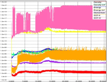
propagation of the IOP wave through the simulation. The residual behavior of the Pathfinder simulation can be seen below in Figure 10 for the second, refined simulation.
Figure 10 - Residuals for Refined ASMAT Pathfinder Simulation
Overall, even after refinement, the simulations exhibited what was considered poor residual drop per iteration for an unsteady simulation. This was particularly true for the density, energy, and momentum residuals, which showed barely an order of magnitude drop for the quickest dropping residuals in both simulations. The exception to this was the SST residuals, which initially showed poor behavior for the 1st simulation, but improved dramatically with the increase in iteration count. The generally poor residual behavior was likely due to a number of factors, including the relatively small number of Gauss-Seidel and Newton-Raphson iterations. To determine areas of poor residual drop within the simulation, and whether targeted refinement might be able to improve their behavior, snapshots of the residuals at the concluding time of the simulation were also obtained and the residual values at mesh locations for density and energy were visualized using iso-surfaces. Iso-surfaces were first created using the maximum residuals for the simulation, and the expansions of these surfaces were captured as the plotted residual thresholds were lowered. Using these methods, it was found that the maximum residual locations were situated at two points in the simulation, which were the inflection point of the nozzle throat contraction and the underside lip of the mushroom deflector.
Residual behavior was further correlated to the CPU memory boundaries within Loci/CHEM to check whether cell allocation in memory was affect residual drop. Loci/CHEM divides cell allocations for the simulation between CPUs based on physical proximity to one another. In prior simulations, it had been noted that regions of high residuals tended to form aligned with these boundaries, which was believed to be due to poor synchronization across CPUs. These analyses showed clear correlations between the CPU boundaries and the density residuals with the region of the trench, but did not extend onto the pad surface. In addition, the correlation did not extend to the energy residuals, which showed no CPU boundary bias. PRESSURE WAVE PROPAGATION AND EVENTS
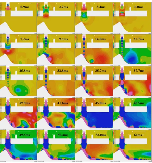
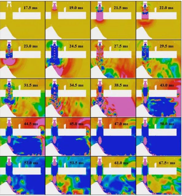
The ASMAT simulations were run for a total of 0.1 seconds with time steps of 0.01 ms for the first case, and 0.02 ms for the second case, which was sufficient to catch most of the major events of the transient startup and progression to a stationary state in both cases. Figure 11 below shows time slices of the pressure for the initial simulation, while Figure 12 shows slices for the refined simulation. These images were created on a cut through the X = 0 plane of the simulation, which ran through the centerline of the rocket. The orange base color represents
atmospheric pressure, red to pink represent oscillations above ambient pressure, and green to blue represent oscillations below it.
Figure 11 - Time Progression of Pressure Waves in Initial Pathfinder Simulation
These two sets of images were roughly correlated based on the flow features noted in the imagery. It was apparent that while the major features were roughly similar in both cases, there were some significant differences in local flow behavior based on the mesh and flow rate changes. Most of these changes were localized to the plume core region, but during the plume start-up phase, they also propagated significantly different waves. The change in flow rate primarily created a delay in the onset of transient features, which averaged out to approximately a 1.4 ms shift over the full simulation.
Figure 12 - Time Progression of Pressure Waves in Refined Pathfinder Simulation
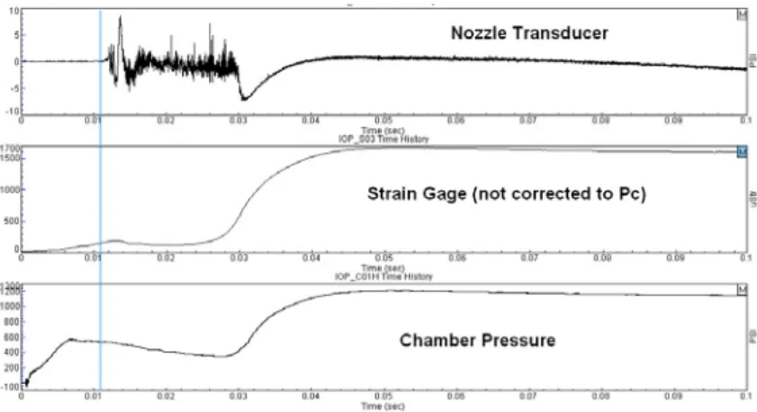
In terms of flow features, there is a dramatic difference in startup behavior between the two simulations. This difference was primarily due to the change in ignition setup. In the first simulation, the pressure of the chamber was directly correlated to the mass flow of the motor. However, in the refined simulation, an attempt was made to model the buildup and delay prior to the loss of the throat plug. Experimental evidence showed that the presence of the throat plug produced a real delay in the onset of pressure propagation in the test hardware. This delayed onset can be seen in Figure 13, which shows the pressure rise rate timing of the motor compared to transducer oscillations in the nozzle for the actual test. Signals didn’t propagate out of the nozzle chamber until after the vertical line in this figure, which was the approximate time when the throat plug was ejected.
Examining this behavior in the simulations, for the initial simulation, beginning at ~1 ms, a pressure wave first escaped from the nozzle and propagated through the simulation for ~ 5 ms; creating an oscillating region of pressure near the launch mount exit for several milliseconds. At ~ 7-9 ms, a shock train began to emerge from the nozzle, having formed off of the contraction in the throat, and proceeded to push the oscillating pressure region of the initial pulse before it down the trench. The shock train took ~7 milliseconds to reach the deflector; and in the process,
compressed the ambient air into a high pressure region at its leading edge. In the refined
simulation, however, nothing happened in the simulation prior ~17 ms, when the loss of the throat plug was triggered. At that point, a strong shock filled the nozzle by ~19 ms, and reached the deflector by ~24 ms.
Figure 13 - Experimental Timing for Nozzle Pressure Rise and Oscillations
A further difference between the two simulations, beyond the throat plug timing, was that the increased resolution below the deck made it so that the miniature shock train never
established itself against the deflector in the refined simulation. In the first, it clearly impacted the deflector, and set up decaying pressure peaks all the way down its length. In the second
simulation, it simply fluttered in the air above the deflector, never quite making contact until the nozzle surged to fully flowing status. A side by side comparison of these features can be seen below in Figure 14.
Figure 14 - Comparison of Initial Pressure Train Behavior between Simulations
At ~32 ms in both simulations, the nozzle began to transition to its fully flowing state. Between this time and ~ 40 ms, the shock train initiation point moved down the nozzle inner surface from the contraction to the lip. At the same time, the shock diamonds within the train expanded as their starting length scale changed. This process reached a head at 40 ms, when the plume had expanded to its maximum size within the plume hole. In the case of the first simulation, at this point it also attached to the walls of the hole. This attached state resulted in rapid, persistent oscillations of flow beneath the hole, and impinging on the deflector, which temporarily broke up the shock diamonds on the deflector; allowing them to reform only at the lip of the deflector or further into the trench. In the case of the second simulation, the changes prohibited the plume from attaching to the wall, and oscillations were never set up under the deck. A side-by-side comparison showing these differences between simulations can be seen in Figure 15.
Figure 15 - Comparison of Plume Behavior Between Simulations
As with the initial shock train formation, the transition to a fully flowing nozzle created several intense pressure buildups as stagnant mass was pushed out of the way of the rapidly expanding plume. While the plume was still attached to the deflector, and before the shock train set up on the trench floor, these pressure waves tended to reflect off the trench floor, and then arc up toward the launch platform. From 35 to 40 ms, the first intense buildup of pressure propagated upward off the floor of the trench and diffracted around the end of the launch platform. This was rapidly followed by a large underpressure pulse, caused by the mass of overpressure air leaving the trench, which filled the whole under-deck volume at ~45 ms and began to diffract around the edge of the launch platform until ~ 50 ms. By this time, the two simulations had become much more correlated in their timing, with a difference of only 1-2 ms between transient features. A time progression showing the evolution of the IOP as it formed and diffracted around the deck can be seen in Figure 16.
Figure 16 - Evolution of Ignition Over-Pressure in Refined Simulation
While these pressure pulses were equilibrating the pressure of the trench, the plume was simultaneously establishing itself along the bottom of the trench floor, and set up a shock train with cells distributed out to the trench exit. By ~ 65 ms, the plume had fully established itself in the trench, and except for some minor oscillations in the space above the plume, remained relatively steady from then on. However, it should be noted that the underpressure region trapped at the edge of the trench exit above the shock train was a steady feature, rather than a transient, and remained present from its formation near 60-70 ms through the simulation period.
PRESSURE SENSOR FREQUENCY EFFECTS
Figure 17 - Used Microphones and Corresponding Probes for the Simulation
Prior to starting the Pathfinder simulation, the locations of physical microphones on the test hardware were determined so that correlations could be performed between real-world data and simulations results. At each location where a real microphone was located, a corresponding recording probe was placed in the simulated environment. The locations of interest for recording were obtained from the ASMAT test group, and were primarily constrained to the IOP series of microphones. The majority of these real-world microphones recorded data at 256,000 samples / sec, with a few exceptions at 4,000 samples / sec (E03 & E04). Naturally, the probes within the simulation space were limited by the timesteps used for calculation, and at best could sample at a rate of 1/timestep. In the first simulation, the probes were recorded at a rate of 1/5 timesteps, with timesteps of 1e-5 seconds, for an effective sampling rate of 20,000 Hz. For the second simulation the probes were recorded at a rate of 1/timestep, but with a longer timestep of 2e-5 seconds, for an effective sampling rate of 50,000 Hz. A visualization showing all of the measured probe locations can be seen below in Figure 17.
For all microphone locations, the ability of the model to resolve high frequency
components in the second simulation was limited to approximately 2500 Hz. This behavior can be seen in a set of example frequency decompositions for microphone locations IOP_093_090H and IOP_M09H, shown in Figure 18 below, where the microphone data is shown in blue, and the
simulated probe data is shown in red. In both data sets, after 2500 Hz, there was a marked loss of correlation between the two datasets, with probe data dropping by nearly 50 decibels over the next several thousand Hz for both cases while data continues out to the expected Nyquist frequency of 25,000 Hz. It should also be noted that the more distant, and lower pressure, case of the T03H microphone appeared to lose correlation earlier, starting to degrade at ~1000 Hz, which was a repeated trend between near- and far-field microphone locations for much of the data.
It is theorized that this rolloff prior to the Nyquist frequency was due to mesh and CFD algorithm related frequency filtering. Operating like spatial aliasing, waves propagating in the simulation were limited by the maximum wavelength the mesh size could support. Waves with lengths shorter than a threshold determined by the cell sizes they travelled through were filtered. This theory appears to be supported by the increased filtering seen by more distant sensor locations, such as those at the top of the tower or vehicle, which rolled off at ~1000 Hz vs the rolloff of nearfield sensors at ~2500 Hz where cell sizes were much smaller.
Figure 18 - Example Frequency Spectra for Microphone and CFD Data
The Loci/CHEM algorithm used a 2nd - Order spatial scheme, the Monotone Upstream-centered Schemes for Conservation Laws (MUSCL), to solve the underlying differential
equations. To solve for subsequent iteration values in a cell, the MUSCL scheme used the value in the cell and the limited flux at the cell edges. However, to build the flux values, it also required the values in nearby cells, so resolving a value in any given cell required at least three cells.
Applying this logic to propagating pressure waves, what was found was that this provided a reasonably accurate correspondence to the frequency filtering seen in results. For a given wave, the shortest wavelength that a cell would be able to resolve was one which spanned it and its two neighbor cells perfectly. Therefore, the wavelength cutoff would be roughly equal to the longest span of three cells that it crossed while travelling from points A to B.
For example, in the ASMAT simulations, much of the IOP signal was propagated up from the trench and through the tower to the vehicle. Examining the cell lengths along this path, it was found that the worst cell lengths were on the order of 0.03 mm. If it was then assumed that three of these cell lengths were required to support construction of one wavelength, then the shortest wave that should be resolved was equal to a 0.09 mm wavelength. Assuming that waves were moving in this simulation at roughly normal sound speed for air (343 m/s), then the best frequency which could be resolved was on the order of ~3800 Hz.
While this example result was close to the actual behavior, this theoretical value was slightly better than the frequency filtering seen in results. However, this theoretical value also represented the best possible frequency resolved from a limited point sampling. While the rolloff started for most nearfield sensors at 2500 Hz, or for farfield at 1000 Hz, the actual frequency amplitudes didn’t generally bottom out until ~5000 Hz. This may have implied that this best case scenario was overly optimistic, and while three cells may have been enough to construct a wave, the amplitudes were so badly degraded for the limit cases as to be non-recognizable at the destination. It may also imply that there were further factors at work reducing the maximum resolved frequency other than pure spatial filtering.
PRESSURE SENSOR COMPARISONS
In the following Figure 19 through Figure 30, comparisons can be seen for each of the microphone locations for the initial and refined simulations, with overlaid plots of the microphone data in blue and the simulation probe data in red. Frequency spectra for each of the pairs of sensor data are also shown side by side with the time domain signals so that range of matched content can be clearly seen. In the interest of space, only six of the 21 possible sensors have been included here, with a sampling taken over a range of locations. Sensors have been shown in pairs of three per page, so that comparisons between the initial and refined simulations can quickly be made.
In terms of time domain data, the initial simulation results already matched most of the major pressure features in both amplitude and timing to within 5-10% error. These values were not improved significantly in the refined simulation. However, for the initial simulations, a number of sensors showed effects from the poor ignition transient modeling, such as spurious oscillations before ignition. These effects were completed removed in the refined simulation, and the
oscillations after the transient were well matched for most sensors. The refined simulations also showed significant improvements for matching of spectral content for both below and above deck content. The range of matched content increased from an average of 1500 Hz in the initial simulations, to approximately 3000 Hz for the refined simulations. Much of this improvement was likely due to the refinements of the below deck and near deck mesh, which resulted in a
INITIAL SIMULATION (093 090, D06, D09)
Figure 19 - Time and Frequency Comparison for Sensor IOP 093 090H (Initial Sim)
Figure 20 - Time and Frequency Comparison for Sensor IOP D06H (Initial Sim)
INITIAL SIMULATION (M03, M09, T03)
Figure 22 - Time and Frequency Comparison for Sensor IOP M03H (Initial Sim)
Figure 23 - Time and Frequency Comparison for Sensor IOP M09H (Initial Sim)
REFINED SIMULATION (093 090, D06, D09)
Figure 25 - Time and Frequency Comparison for Sensor IOP 093 090H (Refined Sim)
Figure 26 - Time and Frequency Comparison for Sensor IOP D06H (Refined Sim)
REFINED SIMULATION (M03, M09, T03)
Figure 28 - Time and Frequency Comparison for Sensor IOP M03H (Refined Sim)
Figure 29 - Time and Frequency Comparison for Sensor IOP M09H (Refined Sim)
SUMMARY AND CONCLUSIONS
Overall, the ASMAT Pathfinder cases showed promising correlation between simulated pressures and real world data in terms of both pressure magnitudes and feature timing. Timings for major peaks of the IOP event appear to be accurate to within a few milliseconds for all microphone locations outside of the launchmount. Timing for higher frequency events was not captured due to apparent spatial filtering of acoustic waves as they propagate over simulation cells too large to sustain them. This lack of correlation can be seen directly from the probe frequency spectra in Figure 53, where there is a visible rolloff in resolved pressures for wave frequencies above 2500 Hz. Amplitude correlation also appears excellent for most probes, with only 5-10% error in matching to pressure peaks for most above and below deck sensors, as well as farfield sensors at elevation. Notable exceptions to this behavior were the launch mount probes, which did not show the significant underpressure of the IOP that was present in the microphone data.
ACKNOWLEDGMENTS
This project was funded by the National Aeronautics and Space Administration (NASA) Marshall Space Flight Center (MSFC) under Jacobs ESTS Contract NNM05AB50C, Task Order 33-000002-CU. Dr. Narayanan Ramachandran was the ESTS Task Lead. Dr. Jeff West (MSFC Fluid Dynamics Branch, ER42) was the NASA Task Monitor.
REFERENCES