No. E2009007
2009-11
Financial Leverage and Market Volatility with Diverse Beliefs
Wen-Chung Guo
1, Frank Yong Wang
2and Ho-Mou Wu
3Abstract:
We develop a model of asset trading with financial leverage in an economy with a continuum of
investors. The investors are assumed to have diverse and rational beliefs in the sense of being
compatible with observed data. We show that an increase in leverage ratio may cause the stock price
to rise in the current period because it increases the demand of optimistic investors through a
“leverage effect”, and will result in “pyramiding” and “depyramiding” phenomena for stock prices in
the subsequent period. Our results also suggest that an increase in leverage ratio also results in an
increase in price volatility as well, however, under certain conditions. Price changes from
pyramiding effect are also negatively associated with margin requirements.Price changes from
depyramiding effect, however, may not be affected when margin calls are not triggered. Furthermore,
the influences of dispersion of opinion, investment funds, and investors’ anticipations are also
examined.
Keywords and Phrases:
Margin Requirements, Differences of Opinion, Stock
Price Volatility, Leverage Effect, Pyramiding/depyramiding
JEL Classification Numbers:
D84, G12, G18
1
Department of Economics, National Taipei University, Taipei, TAIWAN
(e-mail:guowc@ntu.edu.tw)
2
China Center for Economic Research, Peking University, Beijing, CHINA
(e-mail:wangyong9110@pku.edu.cn)
3
China Center for Economic Research, Peking University, Beijing, CHINA
(e-mail:hmwu@ccer.edu.cn)
Financial Leverage and Market Volatility with Diverse Beliefs
Wen-Chung Guo1, Frank Yong Wang2 and Ho-Mou Wu31 Department of Economics, National Taipei University, Taipei, TAIWAN (e-mail: guowc@ntu.edu.tw)
2 China Center for Economic Research, Peking University, Beijing, CHINA (e-mail:wangyong9110@pku.edu.cn)
3 China Center for Economic Research, Peking University, Beijing, CHINA (e-mail: hmwu@ccer.edu.cn)
Nov 14, 2009
Accepted for publication in Economic Theory, 2010.
Abstract: We develop a model of asset trading with financial leverage in an econ-omy with a continuum of investors. The investors are assumed to have diverse and rational beliefs in the sense of being compatible with observed data. We show that an increase in leverage ratio may cause the stock price to rise in the current period because it increases the demand of optimistic investors through a “leverage effect”, and will result in “pyramiding” and “depyramiding” phenomena for stock prices in the subsequent period. Our results also suggest that an increase in leverage ratio also results in an increase in price volatility as well, however, under certain conditions. Price changes from pyramiding effect are also negatively associated with margin re-quirements. Price changes from depyramiding effect, however, may not be affected when margin calls are not triggered. Furthermore, the influences of dispersion of opinion, investment funds, and investors’ anticipations are also examined.
Keywords and Phrases: Margin Requirements, Differences of Opinion, Stock Price Volatility, Leverage Effect, Pyramiding/depyramiding
1
Introduction
The financial sector became highly leveraged before the global financial crisis began in the summer of 2007. The margins (or haircuts) in the repurchase market of various securities were in the range of 1% to 15%, implying a leverage ratio of about 7 to 100 (see IMF (2008)). As for the investment banks involved in the crisis, their leverage ratios were about 20 to 40. Such high leverage ratios were often mentioned as one of main causes for price volatility during the recent episode of dramatic fluctuations. (For related works on the dynamics of recent cycle, see Geanakoplos (2009), Adrian and Shin (2009), and Brunnermeier and Pedersen (2009).) However, the microeconomic mechanism between financial leverage and price volatility has not been thoroughly studied in a general equilibrium framework with heterogenous agents. In this paper we will study an economy with exogenously given margin requirements where speculative trading becomes possible with diverse beliefs as in Kurz (1994, 2009), Kurz and Motolese (2009), Kurz and Wu (1996) and Wu and Guo (2003, 2004).1 Our aim is to develop a general equilibrium model to examine the impact of leverage ratios (or margin requirements) on the level and variation of stock prices.
The relationship between margin requirements and price volatility has also become a major concern in many empirical studies2. In recent years, margin debt relative to the total equity market capitalization has reached a new record high. Many policy makers fear that the rising margin debt might have adverse impacts on overall market performance and volatility.3
Fur-1
Other related works on speculation with heterogeneous expectations include Miller (1977), Varian (1985), Harris and Raviv (1993), Harrison and Kreps (1978), Hart and Kreps (1986) and Morris (1996). In addition to theoretical development, recently empirical studies such as Gao, Mao and Zhong (2003) and Anderson, Ghsels and Juergens (2003) also provide observations of the influence of heterogeneous expectation on asset prices and IPO markets.
2While Moore (1966), Hsieh and Miller (1990) find no significant influence of the margin requirement on price
volatility from the US data, Hardouvelis (1990), Hardouvelis and Peristiani (1992) and Seguin (1990) discovered some negative impacts from an increase in the margin requirement on price volatility. Further, several considera-tions also appear that may affect the reliability in the empirical observaconsidera-tions. First, the margin requirement has been stable since the 1970s, and that the invariability in the margin requirement reduces the power of estimation. Secondly, this observation might have statistical errors because regulators are obliged to increase the margin requirement when volatility increases in the market. Further discussions about the policy debate can be found in Kupiec (1998) and Hardouvelis and Theodossiu (2002).
3
Although the margin requirement has been stable since the 1970s in the U.S., margin debt has increased more than three times faster than household borrowing and overall credit market debt since 1993. During the same period, margin borrowing tripled in relation to gross domestic product. Statistics suggest that margin debt represents approximately 3.6% of disposable income or 1.5% of the total equity market capitalization in the year 2000. Besides this, several large online investment houses had margin debt levels substantially above the overall
thermore, margin trades may contribute to stock price volatility through a dynamic channel. A “pyramiding effect” may occur when stocks continue to appreciate, allowing more borrowing and more stock purchases, which pumps the stock prices higher. On the other hand, there can also be a “depyramiding effect” when prices fall because lenders may issue margin calls and force stock sales, contributing to further stock price plummeting (see, for example, Luckett (1982) and Hardouvelis (1990)).
Although there is a large body of empirical literature on the effects of margin requirements, there are few theoretical conclusions on the emergence of stock price volatility and the role of margin requirements. In an interesting analytical work, Kupiec and Sharpe (1991) developed an overlapping generations model in which there are two types of investors with different risk tolerances. Adopting a two state Markovian framework, they analyzed the particular situation in which margin trading binds in only one of two states. An increase in margin requirements will affect the demand of that particular state and lower its state price. It is shown that there is no unique theoretical relationship between margin requirements and stock price volatility.4
This paper is distinguished from the literature by its emphasis on the role played by specu-lative trading and diverse beliefs. In this paper margin requirements are not restricted to bind only one state as in Kupiec and Sharpe (1991).5 Instead, we adopt a broader approach relying on the heterogeneity of beliefs as in Kurz (1994, 2009) and Wu and Guo (2003, 2004) (also see Miller (1977), Varian (1985, 1989), Harris and Raviv (1993)), which serves as an interesting channel for investigating speculation and price volatility behavior. Recent research dealing with the divergence of opinion has increased, such as Hong and Stein (2003) and Gao, Mao and Zhong (2005). More especially, we find that the effects of a change in asset price due to margin requirements can be decomposed into three components: leverage effects, unbalanced adjust-ment effects and pyramiding/depyramiding effects. We let the leverage effects to represent how a change in margin requirement directly affects the amount investors purchase with leverage. When some investors have margin positions, our framework further considers how stock prices change with the arrival of new information of equilibrium price for the investors. These changes in price are separated into two effects. The first effect, called unbalanced adjustment effects, refers to the case when investors are neither forced or willing to change their balance account. The second effect, pyramiding or depyramiding effect, characterizes the influence when investors
market. 4
Besides this channel of influence in Kupiec and Sharpe (1991), Goldberg (1985) suggested that firms may have incentives to increase their leverage if they act in the best interests of their shareholders who are constrained by margin requirements.
5Coen-Pirani (2005) further points out a binding margin requirement may not affect stock price when investors
have to balance their margin accounts. For instance, a profit (loss) appears after an increase (a decrease) in asset prices, and therefore, investors purchase (sell) shares to balance the account. Furthermore, we demonstrate that an increase in the marginal requirement is anticipated, under a certain set of conditions, to stabilize the markets.
In the next section we present the basic model of stock trading with diverse beliefs. We also demonstrate the existence of an unique equilibrium with speculative trading using margin accounts. The equilibrium stock prices can be characterized using a “marginally optimistic investor,” constructed systematically from the opinion structure of investors. In Section 3 the pyramiding and depyramiding phenomena are shown to exist in our framework. The impacts of the margin requirement and the influence of the belief structure on stock prices are further examined. We show that a more optimistic belief structure is associated with higher stock prices. The heterogeneity of belief is also shown to be positively associated with stock price volatility. Numerical illustrations of the case of unanticipated shocks are presented in Section 4. In Section 5 we extend our model to analyze market volatility when the shocks are anticipated by the investors. Section 6 concludes the paper.
2
The Model with Financial Leverage
The model has three dates (t= 0,1,2) and a risky asset (stock) realizing its final payoff ˜V at date 2. The final payoff ˜V is anticipated to be either high (VH) or low (VL), withVH > VL= 0 for
simplicity to avoid technical complexity. However, the investors in the economy form different opinions about the likelihood of a high payoff. At dates t= 0,1, investors trade on the basis of different opinions. The total supply of shares of this risky asset is normalized to unity. To model a large economy with perfectly competitive markets, let there be a continuum of risk-neutral investors indexed by their types x∈[0,1], the unit interval, as in Aumann (1964, 1966)6.
6In our study the discussions on equilibrium may rely on the marginal investors. Such a framework certainly
depends on the risk-neutrality assumption, which is also adopted in previous studies such as Harrison and Kreps (1978), Harris and Raviv (1993) and Morris (1996). When investors are risk averse, margin requirement may affect the stock trading behavior of only those optimistic investors who have a binding constraint because their wealth is not great enough to purchase their optimal position. The binding constraint argument was previously discussed by Kupiec and Sharpe (1991), who suggested that the effect of a margin requirement on price volatility depends on the state that is binding. If investors are bound in an up state, then an increase in margin requirement will decrease the demand in a good state, that is, a decrease in the price which is higher, and therefore, stabilize the market. The destabilizing argument is similar when investors are bound in a down state. Our framework is different from Kupic and Shape’s because there will always be some investors facing the binding constraints imposed by the margin requirement.
2.1 The Structure of Diverse Belief
In our model each type of investors has a different opinion about the likelihood of high dividends. The typexinvestor has a subjective probabilityB0(x) about obtaining a high payoff
VH and 0 ≤ B0(x) ≤ 1. Putting all individual opinions together, we can identify an opinion
structure{B0(x)}x∈[0,1] for the whole economy. Without loss of generality, we can reshuffle the
investor types so that a higher value for x always corresponds to the more optimistic investor type with a higherB0(x). We assume that the opinion structure has a continuous, differentiable
and monotonically non-decreasing (B00(x) ≥0) function from [0,1] to [0,1]. Here we consider a linear opinion structure B0(x) = a+b·x, with the assumption a ≥ 0 and b > 0 for the
computation, as shown in Figure 1A. The difference between B0(x) and the median opinion
can be used to characterize the extent of differences in investor opinions. We assume that each investor type has an equal number of investors, which is normalized to be equal to one.
[Insert Figure 1 about here]
To simplify this discussion, investors are assumed to have a limited investment fund W0 at
date 0, which is sufficiently large such that default will not occur.
At date t= 1, a random shock occurs to affect investor expectations. The shock is assumed to be unanticipated first and in Section 5 we will extend it to the case of being anticipated. In particular, an up state (u) and a down state (d) are considered for simplicity. Investors become either optimistic or pessimistic at date 1. We assume that the objective probabilities of obtaining a higher final payoff VH for any investor xcan be described as a shift in B0:
Bu(x) = Probu(VH|x) =a+bu·x+u, (1)
Bd(x) = Probd(VH|x) =a+bd·x−d, (2)
where {(bu−b), u} and {(bd−b), d} are the changes in objective probability for each investor,
witha+bu+u≤1,a+bd−d≤1, anda−d≥0 for well-defined probabilities. 7
We assume that at date 0 the initial long margin requirement is exogenous and denoted by
m0, 0< m0 ≤ 1. The margin buyer needs to pay only a proportionm0 of his total purchase.
We do not consider other lending instruments except margin trades. It is assumed that there is
7One may consider a rational learning model to analyze the change in objective probabilities, for example,
with the setting similarly from Teoh and Hwang (1991) and Biais and Gollier (1997). Then Bayesian rule will be applied andBu(x) andBd(x) can be calculated as nonlinear equations. We consider the parallel movement
no default risk, and the parameterm0 is bound away from zero.8
At date 1 optimistic stockholders enjoy capital gains in the up state and therefore increase their positions using margin trades. However, in the down state, those investors suffer a capital loss and consider maintaining a margin mT,mT < m0. The price may either decrease to reach
the maintenance margin or not. If the maintenance margin is triggered, investors will receive a margin call and rebalance their position. Therefore, investors are forced to sell part of their shares to let their position back to the initial margin level. If their positions still have a higher margin than mT, optimistic stockholders will not rebalance their position to maintain greater
positions. Financial institutions serve as the intermediary for margin trading, and we assume that these institutions function in a competitive and frictionless environment. To focus on the essentials, we assume that the riskless rate of return is zero and short sales on the equity are prohibited.
2.2 Asset Market Equilibrium with Margin Requirements
We analyze the equilibria at dates 0 and 1 when the investors speculate by margin trading. In this economy optimistic investors take long position on the stock with margin, and pessimistic ones take a zero position.
For each investor x, at date 0 his investment decision is to consider whether the risky asset is worthwhile related to his subjective valuation. At date 0, if he decides to purchase the asset at equilibrium price p∗0, he obtains the final payoff at date 2. The expected payoff for date 2 is
B0(x)·VH + (1−B0(x))·VL= (a+b·x)VH.
[Insert Figure 2 about here]
The beliefs Bu(x) and Bd(x) at date 1 are described by Equations (1) and (2). Following the
framework of Miller (1977), the willingness to pay for the stock is obviously non-decreasing inx
(since B0(x) =b≥0) and there is a continuum of traders in equilibrium, therefore a “marginal optimistic investor”x∗0 must exist (illustrated in Figure 1) such that the willingness of investor type x∗0 to pay is equal to the equilibrium pricep∗0 at date 0:
p∗0 =B0(x0∗)·VH + (1−B0(x∗0))·VL= (a+b·x∗0)VH . (3)
For investors of type x ∈ [x∗0,1], their willingness to pay is higher than the equilibrium price. These investors will purchase stock on margin. The market clearing condition can be written as
E0 = (1−x∗0) W0 p∗0 1 m0 −1 = 0, (4) 8
A sufficient condition to prevent the default from occurring at date 1 is that the price at down state is greater than (1−m0) multiplying the price at date 0.
whereE0 is denoted as the excess demand for this risky asset, because optimistic investors will
use all of their wealth to purchase stocks on margin, given initial holding shares as θ0(x) =
W0/(p∗0m0). The above equations could be rewritten as
p∗0 = (1−x
∗ 0)W0
m0
,
which is a strictly decreasing function of x∗0. From (3) we can derive following equations:
p∗0 = W0(a+b)VH
W0+bm0VH
, x∗0 = W0−am0VH
W0+bm0VH
. (5)
Our model provides a framework in which investor opinion essentially determines the price of the equity. Usually investors buy a stock when they believe it is a good investment, and therefore, their demand drives the stock price up. However, if investors think the outlook for this project is poor, they either do not invest or sell the shares that they already own, and as a result the stock price will fall. The stock becomes more valuable because there is demand for it. The short sales constraint assumption is also adopted from Harrison and Kreps (1978), Ku-piec and Sharpe (1991), Harris and Raviv (1993) and Morris (1996). However, this assumption can be easily relaxed in our framework. If investors are allowed to sell short with margin re-quirement ms, then those pessimistic investors who originally did not hold any stock will take
a short position, resulting in additional supply. The market clearing condition of (4) can be extended in this framework as
(1−x∗0)W0 p∗0 1 m0 −1−x∗0W0 p∗0 1 ms = 0,
where the third item indicates the aggregated short position. Since allowing short sales induces additional supply, the asset price will decrease. In practice, however, trading by selling short is less observed than margin trading, because of either regulations, optimism or the fears of investors.
At date 1, either the up stateuor down statedis realized and all investors adjust their beliefs on the project as (1) and (2). Let p∗u and p∗d be the equilibrium prices for the up and down state, respectively. When the up state occurs, investors become more optimistic. Therefore, the demand for the equity increases, and as a result, the stock price increases, i.e., p∗u > p∗0. Therefore, for those investors x > x∗0, their wealth increases to
Wu(x) = W0 p∗0 1 m0 p∗u−( 1 m0 −1)W0> W0,
because they make capital gains from trading on margin. In this equation the first item is the position value which is equal to θ0p∗u. The second item is the borrowing on margin. The
optimistic investors (x ≥ x∗u) has θu(x) = Wu(x)/(m0p∗u) shares of stock and the equilibrium
conditions (3) and (4) become
p∗u=Bu(x∗u)·VH + (1−Bu(x∗u))·VL= (a+b·x∗u+u)VH , (6) Eu = (1−x∗u) 1 m0 Wu(x) 1 p∗u −1 = (1−x ∗ u)W0 1 m0 ( 1 m0 1 p∗0 −( 1 m0 −1)1 p∗u)−1 = 0, (7)
whereEu is the excess market demand. From (3) and (4) we have the equilibrium:
p∗u = (a+b·x∗u+u)VH , (8) where x∗u = −k2− p k2 2 −4k1k3 2k1 , (9)
is a solution to the following quadratic function:
k1x2u+k2x2u+k3 = 0, (10) where k1 = 1 m2 0 W0 p∗0 bVH , k2 =bVH−VH 1 m20 W0 p∗0 (a+u+b) + ( 1 m20 − 1 m0 )W0, k3 = (a+u)VH −VH 1 m2 0 W0 p∗0 (a+u) + ( 1 m2 0 − 1 m0 )W0.
The stock price decline case is different from the previous. When the stock appreciates, margin traders can withdraw from the margin account and use it to buy additional stock. However, if the price depreciates, margin traders are not required to add funds to their margin account unless the margin calls are triggered (see Hardouvelis and Theodossiu (2002) for details). When a down state (d) is observed at date 1, all investors become more pessimistic. The demand for the equity decreases because each investor adjusts the expected value of the equity to less valuable. For those investors x > x∗0, their wealth decreases to
Wd(x) = W0 p∗0 1 m0 p∗d−( 1 m0 −1)W0< W0.
Therefore, it can be shown that the stock price decreases, i.e.,p∗d< p∗0. In the down state, there are two possible outcomes, depending whether margin calls are triggered. If a decrease in price results in a loss such that the margin is still greater or equal to the maintenance margin, that is,
m0p∗0−(p∗0−p∗d)
p∗d ≥mT ,
which can be rearranged as follows:
m0(a+bx∗0)VH −((a+bx0∗)VH −(a+bx∗0−d)VH)
(a+bx∗0−d)VH
and leads to the following inequality:
d≥d∗m = (m0−mT)(a+bx∗0)/(1−mT). (11)
It is mentioned that The trigger point d∗m is negatively associated with mT since∂d∗m/∂mT = −(a+bx∗0)(1−m0)/(1−mT)2<0. In this case stockholders will not sell their shares, because
their position will decrease if they rebalance their position. The equilibrium stock price becomes
p∗d=Bd(x∗0)·VH + (1−Bd(x∗0))·VL= (a+b·x∗0−d)VH , (12)
In the circumstance when a margin call is triggered, however, investors are forced to rebalance their position to the level of the initial marginm0. Those investorsx > x∗0 who purchase equities
at period 0, however, suffer short-term capital losses. It can also be shown later that the marginal investors x∗d shall be less than x∗0. Since all investors become pessimistic and those investors
x > x∗0 suffer a loss of wealth, as the price decreases, some of those investors that do not own stock at period 0 may use their available funds to purchase that stock. Their types are
x ∈ [x∗d, x∗0), so they have x∗0 −x∗d population. Henceforth, the equilibrium conditions (3) and (4) become p∗d=Bd(x∗d)·VH + (1−Bd(x∗d))·VL= (a+b·x∗d−d)VH , (13) Ed= (x∗0−x∗d)(W0) 1 m0 1 p∗d + (1−x ∗ d)Wd(x) 1 m0 1 p∗d −1 = 0. (14)
The later equation is calculated as
Ed= (x∗0−x∗d)(W0) 1 m0 1 p∗d + (1−x ∗ 0)W0 1 m0 ( 1 m0 1 p∗0 −( 1 m0 −1)1 p∗d)−1 = 0, (15)
whereEdis the excess market demand. It is further assumed that W0 is large enough to avoid
the degenerated case x∗d≤0. By further calculations we obtain the equilibrium:
x∗d= W0[p ∗ 0(2m0x∗0−m0−x∗0+ 1)−(1−x∗0)(a−d)VH] +VHp∗0m20(a−d) p∗0m20VHb+W0(p∗0m0+bVH(1−x∗0)) , (16) p∗d= W0p ∗ 0VH[(a−d)m0+b(2m0x∗0−m0−x∗0+ 1)] p∗0m20VHb+W0(p∗0m0+bVH(1−x∗0)) . (17)
Here we establish our first result:
Proposition 1 (Existence and uniqueness of the equilibrium): An unique equilibrium exists in the economy with margin requirements when there are differences of opinion {p∗0, x∗0, p∗u, x∗u, p∗d, x∗d}, which satisfies that p∗d< p∗0< p∗u, x∗d< x∗0 < x∗u.
Proof: The existence and uniqueness of p∗0, x∗0, p∗u, xu∗, p∗d, x∗d is solved uniquely. p∗0 < p∗u
demands of shares θu(x) increase for those investors x ≥ x∗0 who have capital gains from the
increase in stock price. Using the market clearing condition (1−x∗u)θu = 1, we can prove that
x∗u > x∗0. The property ofx∗d and p∗d can be proved similarly.
The above property demonstrates how the expectation adjustment among investors may affect stock prices. At date 1, if an up shift in expectation (u) is observed, an increase in demand occurs and pushes the price up. Conversely, the price will fall as the down state (d) is observed. This result illustrates that a change in expectation may induce greater volatility.
3
Market Volatility and the Influences of Margin Requirements
The previous theories in Luckett (1982) and Kupiec and Shape (1985) focused on the credit aspect, that is, the effects of margin requirements are reductive if the credit constraint is not bind-ing (their optimal leverage is not relatively large). However, the pyramidbind-ing/depyramidbind-ing phe-nomenon is not fully analyzed. In contrast, this paper provides a framework to discuss the effects of margin requirements. We decompose it into “leverage effect” and pyramiding/depyramiding effect. A change in the margin requirement initially influences the credit for purchasing stocks. A simple example may help illustrate these two effects. Consider that an investor with $1000 may purchase the stock at most $2000 or 50% margin. If the margin decreases to 40%, the credit increases to $2500. That is, there is an additional $500 of free credit for investments, namely the leverage effect. Assume that in the next period the price either increases or decreases 10%. When the price goes up, the investor enjoys a capital gain of $200 and may purchase additional shares, keeping the margin requirement satisfied. An increase in additional cash from capital gain may push the price higher, called the pyramiding effect. Conversely, the investor suffers a loss when the price goes down, and is required to decrease their position to satisfy the margin requirement. The price may decrease further, called the depyramiding effect.
The above example intuitively suggests that a decrease in margin requirement results in a positive effect on the initial stock price. However, when the asset moves from the original level, before the margin call occurs and the investors rebalance their credit, we call it a leverage effect in this paper. However, investors may change their positions due to a capital gain or loss. If the stock price increases, because the investors have additional credit to purchase new shares and maintain the margin requirement, the stock price may increase further. This phenomenon is called the pyramiding effect. Conversely, the depyramiding effect describes the case when investors suffer a loss from stock depreciation and then reduce their position. Hence, the stock price decreases further. While the above argument is accepted for the margin requirement
discussion, the effect of stock prices in a general equilibrium is more complicated. For instance, a decrease in margin requirement results in an increase in initial price, and therefore, reduces further capital gain given the same future price.
3.1 Leverage Effect and Static Results
We first discuss the current equilibrium stock price. The static result of a margin requirement here is consistent with the previous single-period models in Goldberg (1985) and Luckett (1982). The following two propositions discuss how changes in several parameters may affect the current equilibrium stock price at date 0.
Proposition 2 (Leverage effect on the current stock price): Equilibrium price p∗0 is negatively related to the margin requirement m0.
Proof: It is simply observed from
∂p∗0/∂m=−VH2W0(a+b)b/(m0bVH +W0)2 <0.
In the result above, an increase in the margin requirement restrains the leverage that investors may use, and therefore, decreases the stock demand and the current equilibrium price falls.
Proposition 3 (Comparative statics on the current stock price): The current equilibrium price
p∗0 is positively related to W0,VH, a, andb.
Proof: It is proven using the following comparative statics:
∂p∗0/∂W0=VH2(a+b)m0b/(m0bVH+W0)2>0,
∂p∗0/∂VH =W0(a+b)2/(m0bVH +W0)2 >0,
∂p∗0/∂a=VHW0/(m0bVH +W0)>0,
∂p∗0/∂b=W0VH(W0−m0VHa)/(m0bVH+W0)2>0.
The effect of available investment funds reflect the cash environment. When the available fund is higher, optimistic investors have greater wealth to purchase, which boosts the equilibrium price. It also provides some implications for the monetary policy effects on the capital markets. It suggests that when an expansionary monetary policy or more investment funds are injected into a speculative market, the optimistic investors will put more cash into the market and therefore
boost the prices higher. The equilibrium price is also positively related to the final payoff because of the market fundamentals. Moreover, the equilibrium price increases as investors become more optimistic.
Proposition 4 (Pyramiding/depyramiding): Pyramiding always occurs in the equilibrium when the up state occurs, that is,p∗u is greater than the unbalanced priceBu(x∗0)·VH+(1−Bu(x∗0))·VL.
However, depyramiding occurs only when the down change is large enough to result in margin calls, i.e., d > d∗m = (m0−mT)(a+bx∗0)/(1−mT). In the depyramiding case, p∗d is less than
Bd(x)·VH + (1−Bd(x))·VL.
Proof: Pyramiding occurs becausex∗u > x∗0, which results inp∗u=Bu(xu∗)·VH+(1−Bu(x∗u))·VL>
Bu(x∗0) ·VH + (1−Bu(x∗0))·VL. The price in the down state is observed in (13) and (14).
Therefore, depyramiding appears only when the down change in expectation is large enough to
trigger margin calls.
The asymmetrical result is found in empirical observations in Hardouvelis and Theodossiou (2002). They point out the asymmetric property of pyramiding/depyramiding effects that a margin requirement is more effective in a bull market and less significantly effective in a bear market. Our results further suggest that the depyramidin effect may occur significantly when the down change in price is greater, causing margin calls.
3.2 Influence of Changes in Margin Requirements
Because a change in margin requirement may result in impacts in leverage and pyramd-ing/depyraiding as well, we decompose these three effects as follows. The leverage effect of margin requirements on the subsequent stock prices is examined first. Denote Fs, as “
unbal-anced stock price,” as the willingness to pay at states,s=u, d, representing when investors do not rebalance their margin account:
Fu =Bu(x∗0)·VH + (1−Bu(x∗0))·VL= (a+bx∗0+u)VH ,
Fd=Bd(x∗0)·VH + (1−Bd(x∗0))·VL= (a+bx∗0−d)VH ,
It leads to:
Fu(x)−Fd(x) = [Bu(x∗0)−Bd(x∗0)]·(VH −VL) = (u+d)x∗0VH .
When the up state occurs, from (7) the stock price can be described as
p∗u=Fu(x∗0) + (p ∗
The first item in the right part of the above equation can be indicated as the leverage effect which does not consider a further increase or decrease in credit. It simply describes the stock price when further adjustment in a position is not allowed. The second item, however, is the pyramiding effect. Similarly we have the equation in the down state:
p∗d=Fd(x∗0)−(Fd(x∗0)−p ∗
d). (19)
The leverage and depyramiding effects are the first and second items in the right part of the above equation.
From this setting we can analyze the pyramiding/depyramiding effects. The pyramiding effect (p∗u−Fu(x∗0)) represents that investors rebalance their credit using capital gains to purchase
more shares. Conversely, the dyramiding effect (p∗d−Fd(x∗0)) represents that the investors reduce
their position further because of a capital loss. We represent pyramiding and depyramiding effects as follows.
p∗u−Fu(x∗0) = [VL+Bu(x∗u)·(VH −VL)]−[VL+Bu(x∗0)·(VH −VL)] = (x∗u−x∗0)bVH, (20)
Fd(x∗0)−p∗d= [[VL+Bd(x∗0)·(VH −VL)]]−[VL+Bd(x∗d)·(VH −VL] = (x∗0−x∗d)bVH. (21)
We further decompose the margin requirement effect on asset price volatility into three compo-nents: p∗u−p∗d= [Fu(x∗0)−Fd(x∗0)] + (p ∗ u−Fu(x∗0)) + (Fd(x∗0)−p ∗ d), (22)
The leverage effect results are described as follows:
Proposition 5 (Influence of Margin Requirements on Unbalanced Stock Prices): An increase in margin requirementmresults in a negative leverage effect on the stock price (p∗uandp∗d). With the assumption of parallel movement in the opinion structure, the unbalanced stock volatility is not associated with a margin requirement. That is,
1. ∂Fs(x∗0)/∂m <0, s=g, b, 2. ∂[Fu(x∗0)−Fd(x∗0)]/∂m= 0 .
Moreover, Fs(x∗0), s=u, dare positively related to W0, VH, a, and b.
Proof: It is proven obviously byFu= (a+bx∗0+u)VH andFd= (a+bx∗0−d)VH and Proposition
2.
The above result suggest that for the leverage effect, an increase in margin reduces the credit investors can use, and therefore, decrease the stock price. However, because of the parallel shift
in expectation in our framework, a margin requirement does not influence price volatility with the assumption of parallel movement. In a more general framework one can consider a general shift in expectation, then how that shift in expectation may affect the equilibrium.
Proposition 6 (Influence of Margin Requirements on Pyramid/Depyramiding Changes): An increase in margin requirement results in a positive (negative) effect on pyramiding or depyra-miding if the stock ownership becomes more (less) concentrated. That is, That is,
1. ∂[p∗u−Fu(x∗0)]/∂m0 <0, if ∂(x∗u−x∗0)/∂m0<0 , 2. ∂[Fd(x∗0)−p∗d]/∂m0 <0. if ∂(x∗0−x∗d)/∂m0 <0 .
Proof: It is obvious from (19) and (20).
Proposition 7 (Influence of margin requirements on stock prices): The equilibrium price p∗u is decreasing related to the margin requirement m, i.e., ∂p∗u
∂m0 <0, and p
∗
d is decreasingly related to
the margin requirement m0 if the change in margin requirement is small anddnot large enough to trigger margin calls, that is, ∂p
∗ d ∂m0 <0. Proof: ∂x∗u ∂m0 ≥0 if ∂p∗u ∂m0 ≥0. From ∂x∗0
∂m0 <0 it leads to a contradiction (to be checked in detail ).
Becausex∗d=x∗0 when margin calls are not triggered, and using Propositionx∗0 is negatively re-lated withm0, it then suggests thatx∗dandp∗dare negatively associated withm0.
This proposition suggests that an increase in the margin requirement mreduces the amount of speculation by optimistic investors, therefore prices decline as favorable information is ob-served. Hardouvelis (1990) provided empirical evidence on the margin requirements effect on stock market volatility to examine the pyramiding/depyramiding effect argument. This paper, however, demonstrates how the pyramiding effect may arise in a theoretical model with specu-lative trading and margin requirements.
The next result summarizes the margin requirement effect on the price volatility.
Proposition 8 (Influence of Margin Requirements on Price Volatility): An increase in margin requirement m results in a positive (negative) effect on price volatility if the stock ownership becomes more (less) concentrated. That is,
Proof: This is proven using Propositions 5 and 7.
This proposition suggests that an increase in the margin requirement mreduces the amount of speculation by optimistic investors, therefore prices decline as favorable information is ob-served. Hardouvelis (1988, 1990) provided empirical evidence on the margin requirement effect on stock market volatility to examine the pyramiding/depyramiding effect argument. This pa-per, however, demonstrates how the pyramiding effect may arise in a theoretical model with speculative trading and margin requirements.
4
Comparative Statics of Market Volatility with Unanticipated
Shocks
In the framework we have studied so far, the investors at date 0 do not anticipate the possible changes of beliefs described by Equations (1) and (2). Therefore, they compute the payoffs according to Equation (3) and do not purchase stocks to benefit from intermediate trading at date 1. This is called the case of unanticipated shocks.
4.1 The Effects of Margin Requirements
First we present an example for the margin requirement effect on the equilibrium. It shows that equilibrium prices are negatively associated with the margin requirementm, and so is price volatilityp∗u−p∗d. This result can be compared to the literature on speculation and volatility.
Example 1: We consider a set of parameters VL = 10, VH = 20, W0 = 20, opinion structure
B0(x) = 0.25 + 0.5x, u = d = 0.25, and maintenance margin mT = 0.5·m0. In Proposition
7 we analyze the margin requirement impact on prices p∗u, and p∗d. The example as shown by Table 1 illustrates negative associations between them. Pyramiding (p∗u−Fu) and dypyramiding
(Fd−p∗d) are also shown in Table 1. In Figure 3 we illustrate how price volatilities, pyramding and
depyramiding are negatively associated with margin requirements. A greater shock (u = d = 0.25) provides greater volatility and pyramiding/depyramiding effects. Moreover, the margin requirement impact on p∗d is smaller than it on p∗u. Therefore, the price volatility decreases in
m0.
Example 1 demonstrates the presence of destabilized speculation when margin requirements increase. This result provides a theoretical explanation of speculative trading on several relative empirical evidences observed in the US and other markets (see, for example, Hardouvelis (1990)
and Hardouvelis and Peristiani (1992)). It should also shed light on a policy issue. If the government sets out to cool a overheated stock market, a increase in margin requirement may pull the prices down and reduce stock price volatility. However, if the government wants to spur on an undervalued stock market, a decrease in margin requirement may push prices up and increase stock market volatility.
[Insert Table 1 about here] [Insert Figure 3 about here]
4.2 The Effects of Dispersions of Opinion
With a similar set of parameters given thatVH = 20, VL= 0,W0 = 20,B0(x) = 0.25 +b·x,u=
0.2,d= 0.25, and maintenance marginmT = 0.5·m0. Figure 4 discusses how opinion dispersion
may affect price volatility (p∗u−p∗d), pyramiding (p∗u−Fu(x∗0)) and depyramiding (Fd(x∗0)−p∗d).
Generally the price volatility, pyramiding and depyramidig are positively associated with opinion dispersion, except in the case when depyramiding moves from positive to zero.
[Insert Figure 4 about here]
Figures 4A and 4B suggest that both price volatility and pyramiding increase as opinion disperses among investors. Depyramiding, as shown in Figure 4C, however, may decrease when depyramiding becomes zero, that is, when margin calls are not triggered. The intuition behind this result is that the marginal investor is relatively optimistic when the price is relatively high, making the heterogeneity of opinion structure enhance optimism and increase stock prices when an up state is observed. The marginal investor plays an important role in characterizing the equilibrium properties. This result can be compared to Miller (1977), who provided a simple two-period model for studying the divergence of opinion and argued that an increase in the di-vergence of opinion will increase market prices because a minority of investors absorb the entire security supply. Besides confirming Miller’s result (1977) we also obtain a complete characteri-zation. The price p∗d, however, decreases in the dispersion of beliefs, because the heterogeneity of beliefs may enhance marginal investor pessimism and reduce stock prices. In the table we can find that price volatility is positively related to the dispersions of opinion among investors.
4.3 The Effects of Investment Funds
Figure 5 illustrates the impact of margin requirements on price volatility (p∗u−p∗d), pyramiding (p∗u−Fu(x∗0)) and depyramiding (Fd(x0∗)−p∗d), given the parametersVH = 20, VL= 0, B0(x) =
0.25 + 0.5·x,u = 0.2, d= 0.25, and maintenance margin mT = 0.5·m0. The price volatility,
pyramiding and depyramidig are in general negatively associated with investment funds. In Figure C, dypyramiding is 0 when m0 = 0.8. The amount of investment funds is positively
associated with the stock prices, but negatively associated with price volatility. This result may explain the phenomenon that an increase in money invested in the market may lead to positive market returns. Our result may also be compared to the monetary policy issue. It is suggested that a loose monetary policy may be helpful for equity market performance, while a tight monetary policy tends be negatively associated with market performance.
[Insert Figure 5 about here]
5
Market Volatility with Anticipated Shocks
In this section, the model setup is the same as that of Section 2 except that all investors anticipate there will be a shock affecting their expectations at t = 1. For simplicity, let bu =
bd = b. Thus for all investors, B0(x) = u+ddBu(x) + u+udBd(x). That is to say, at t = 0 all
investors are aware that an up state will be realized att= 1 with the same probability, although they have different opinions when the state is realized. Let θ = u+dd denote the probability of the up state.
5.1 Leveraged Trading with Speculations
Given the stock price P0 and ˜P1 (including Pu and Pd), investors at date 0 choose their
demandsD0(x) and ˜D1(x) (includingDu(x) and Dd(x)) to maximize their expected wealth:
˜ W(x) =W0+D0(x) ˜P1−P0 + ˜D1(x) ˜V −P˜1 .
Because the shock is anticipated by all investors, backward induction is applied. At t = 1, the analysis is just the same as in Section 2 since there is no more trading opportunities. There exist critical values xu and xd ∈ (0, 1) (marginally optimistic investor) such that equilibrium
prices are characterized as follow:
Pu=Bu(xu)VH = (a+bxu+u)VH, (24)
Pd=Bd(xd)VH = (a+bxd−d)VH. (25)
Investors who are more optimistic than the marginally optimistic investor buy the stock on margin, and those who are more pessimistic are inactive in the market. When the up state is realized, for investors who are more optimistic, i.e., x > xu, their wealth become Wu(x) =
W0+D0(x)(Pu−P0)> W0, and the market clearing condition is
R1
xu
Wu(x)
m0Pudx= 1.
But things become more complicated when the down state occurs. Investors who buy the stock at date 0 suffer from a capital loss. For investors who are more optimistic than xd and
purchase stock at date 0, when m0P0−(P0−Pd)
Pd < mT(or, mT > 1−
P0
Pd(1−m0): maintenance
margin is close to initial margin), margin calls are triggered, and they have to rebalance their position to the initial margin level. Therefore for those investors,Dd(x) = Wmd0(Pxd), otherwise they
continue to hold D0(x). However, for investors who are more optimistic than xd and do not
purchase stock at date 0, there is no problem of margin call , thus Dd(x) = mW0P0d.
Next we study investors’ demand at date 0. By backward induction, investors know that ˜D1
are functions ofD0. The optimal demandD0(x) is chosen to maximize investors’ expected final
wealth: E˜ W(x) =W0+D0(x) θPu+ (1−θ)Pd−P0 + θDu(x) (Bu(x)VH −Pu) + (1−θ)Dd(x) (Bd(x)VH−Pd) . (26)
Given the equilibrium prices P0, Pu, Pd and let E(P1) = θPu + (1−θ)Pd, E[ ˜W(x)] is a linear
function of period 0’s demand for all investors, so investors will purchase stock as much as they can att= 0, or D0(x) =W0/m0P0 if and only if
∂E[W˜(x)]
∂D0 ≥0; otherwise they will not buy any
stock.
For the most pessimistic investors x <min{xu, xd}:
E[ ˜W(x)] =W0+D0(x) E(P1)−P0
. (27)
If P0 ≤ E(P1),
∂E[W˜(x)]
∂D0 = E(P1)−P0 ≥ 0, implying that they will purchase the stock on
margin, even though they don’t hold any stock at t = 1. According to Kaldor (1939), they are the “speculators” who purchase the stock at date 0 with the purpose to sell it at date 1. However, if Pd<E(P1)< P0 < Pu, for these investors who are most pessimistic,
∂E[W˜(x)]
∂D0 <0,
thus they hold zero position at both t= 0 and t= 1.
Following we look for equilibria withPu > Pd, especially those equilibria withPu> P0 > Pd.
exclude the trivial case where P0 ≤ Pd at equilibria, we assume that investors have enough
fund.9 But there are two kinds of equilibria, one with Pd < P0 ≤E(P1) < Pu, the other with
Pd < E(P1) < P0 < Pu. We will focus on the former case where speculation is present, the
analysis of the later case can be found in Appendix A.
5.2 The Properties of Equilibrium Prices
When Pd < P0 ≤ E(P1) < Pu, the most pessimistic investors x < min{xd, xu}
pur-chase stocks for speculation. Following we look for a specified equilibrium where investor
x∈(0, x0) (x0 >max{xd, xu}) purchase stock att= 0. Other kinds of equilibrium are discussed
in Appendix B.
Following let’s just ignore maintenance margin condition for a moment. If xu > xd, the first
derivative of investors’ expected wealth with respect to their demand at t= 0 is:
∂E h ˜ W(x) i ∂D0 = E(P1)−P0+θPmu0−PPu0(x−xu)bVH+ (1−θ)Pmd−0PP0 d (x−xd)bVH,ifx≥xu, E(P1)−P0+ (1−θ)Pmd−0PP0 d (x−xd)bVH,ifxd≤x < xu, E(P1)−P0,ifx < xd. (28) And when ∂E[∂DW˜(x)] 0 x=x u > 0 and ∂E[∂DW˜(x)] 0 x=1
< 0, there exists x0 > xu such that ∂E[W˜(x)] ∂D0 x=x0 = 0.
[Insert Figure 6 about here]
And if xu< xd, the first derivative is:
∂EhW˜(x)i ∂D0 = E(P1)−P0+θPmu0−PPu0(x−xu)bVH + (1−θ)Pmd−0PPd0(x−xd)bVH,ifx≥xd, E(P1)−P0+θPmu0−PPu0(x−xu)bVH,ifxu≤x < xd, E(P1)−P0,ifx < xu. (29) Since Pu > E(P1) > P0, ∂E[W˜(x)] ∂D0 x=xd
must be positive, and when ∂E[∂DW˜(x)]
0 x=1 < 0, there existsx0> xd such that
∂E[W˜(x)] ∂D0 x=x0 = 0. 9
It can be shown that there exists an unique equilibrium withPu> Pd> P0 whenW0/m0≤(a−d)VH. We
[Insert Figure 7 about here]
Due to linearity, investors purchase stock on margin if and only if the first derivative of expected wealth to demand is positive. The conditions for equilibria are stated below no matter whether xu ≥xd orxu< xd: 1. x0 W0 m0P0 = 1, (30) 2.(x0−xd) W0 m0P0(Pd−P0) m0Pd + (1−xd) W0 m0Pd = 1, (31) 3.(x0−xu) W0 m0P0(Pu−P0) m0Pu + (1−xu) W0 m0Pu = 1, (32) 4. ∂E ˜ W(x) ∂D0 |x=x0 = E(P1)−P0+θ Pu−P0 m0Pu bVH(x0−xu) + (1−θ) Pd−P0 m0Pd bVH(x0−xd) = 0, (33) 5. max{xu, xd}< x0 <1, Pd P0 < 1−m0 1−mT, (34)
where Equation (30) is the market clearing condition at date 0, Equations (31) and (32) are the market clearing conditions of the down and up state at date 1, respectively. x0 is determined
by Equation (33), and Equation (34) is the feasible and maintenance margin condition.
Next we present an example to show the impact of margin requirement on stock prices level and volatility. It is shown that the price level P0, Pu and Pd are all decreasing with margin
requirement. However, the price volatility, measured by Pu−Pd does not vary monotonically
with margin requirement, which is different with the case of unanticipated shock.
Example 2: Suppose that a=u=d= 0.1, b= 0.4, VH = 10, W0 = 1, mT = 0.8m0, so θ= 0.5,
and Pu = 2 + 4xu, Pd= 4xd.
We can check that when m0 = 20%,
xu = 0.4459< xd= 0.4899< x0= 0.5666, and prices: Pd= 1.9595, Pu= 3.7834, P0 = 2.8328, constitute an equilibrium. And when m0 = 50%, xd= 0.1914< xu = 0.3348< x0= 0.6792, and prices: Pd= 0.7656, Pu= 3.3392, P0 = 1.3585,
constitute an equilibrium.
There existsm0 = 22% such that whenm0 > m0,xd< xu at equilibrium, otherwisexu < xd.
The prices level decreases with margin requirement, or increases in leverage ratio, which is very intuitive: the higher leverage ratio, the more leveraged fund the investor can invest in stock, and more demand drives the stock price up. But the impact of leverage ratio on up state and down state price are asymmetric, and we can get the economic reasons from the changes of
xu and xd. Both xu and xd decrease with margin requirement, and there exists m∗0 (= 45% in
Example 2) such that when m∈ m0, m∗0,xd decrease with margin requirement more quickly
than xu, and when m > m∗0, xu decrease more quickly than xd. Since ∂(P∂mu−0Pd) ∝ ∂(x∂mu−0xd),
therefore price volatility increases with margin requirement when margin level is relative low, and decreases with it when margin is relative high. Therefore, a reduction in leverage ratio may not lead to lower price volatility.
[Insert Table 2 about here]
6
Concluding Remarks
This paper developed a theoretical framework to analyze the impacts of adjusting margin requirements on market prices and volatilities in the presence of diverse opinion and speculative trading on margin. Margin trading is demonstrated to enhance speculation and stock price volatility in our model because investors can obtain additional funds to finance their strategies. Pyramding/depyramiding effects were illustrated. Dispersion of opinion increases the price in a good state but decreases the price in a down state. The effects of investment funds and policy implications were also discussed. Furthermore, we demonstrate that when the shocks are anticipated the investors may engage in speculative trading and a reduction in leverage ratio may not reduce price volatility.
The pyramiding/depyramiding effects analyzed by this paper will be clearer in an extended framework with multiple periods. Consider the framework with T dates of trading and final payoff realizing at date T + 1, in which there observes identical and independent signals are observed at each date between 2 and T−1. We can then solve the equilibrium using iterations similar to equations (5)-(8) with nonlinear computations. The pyramiding mechanism is still observed because when an up state is observed, investors purchase more stocks because they are profiting from margin trading and rebalancing their positions, and therefore the stock prices increase. The depyramiding effect, however, may not be observed when the margin calls are not
triggered.
Although the impacts of reducing leverage ratios are often believed to be stabilizing the market, our study demonstrates that such a belief still needs to have a stronger foundation in theory. Further studies with risk averse investors and sophisticated trading strategies are needed to clarify this issue.
References
[1] Anderson, E.W., Ghsels, E. and Juergens, J.L. :Does Heterogeneous Beliefs Matter for Asset Pricing? Review of Financial Studies,18, 875-924 (2003)
[2] Arrow, K. J., “Le Rˆole des valeurs boursi`eres pour la repartition la Meilleure des risques.
´
EconometrieC.N.R.S.,40 41-47 (1953) Translated as :The Role of Securities in the Optimal Allocation of Risk Bearing. Review of Economic Studies 31, 91-96 (1964)
[3] Aumann, R. J.: Markets with a Continuum of Traders. Economtrica 32, 39-50 (1964) [4] Aumann, R. J.: Existence of Competitive Equilibrium in Markets with a Continuum of
Traders. Economtrica34, 1-17 (1966)
[5] Biais, B. and Gollier, C.: Trade Credit and Credit Rationing. Review of Financial Studies
10, 903-937 (1997)
[6] Borts, G.H.: Agenda for a Commission to Study Financial Markets, Their Structure, and Regualtion. Journal of Money, Credit and Banking 3 , 2-6 (1971)
[7] Brunnermeier, M. and Pedersen, L.: Market Liquidity and Funding Liquidity, Review of Financial Studies,22(6), 2201-2238 (2009)
[8] Coen-Pirani, D.: Margin Requirements and Equilibrium Asset Prices. Journal of Monetary Economics52, 449-475 (2005)
[9] Feiger, G.: What Is Speculation. Quarterly Journal of Economics 90, 677-87 (1976) [10] Fostel, A. and Geanakoplos, J.: Leverage Cycles and the Anxious Economy, American
Economic Review, 1211-1244 (2008)
[11] Gao, Y., C. Mao and Zhong, R.: Divergence of Opinion and Long-Term Performance of Initial Public Offerings. Journal of Financial Research29, 113-129 (2005)
[12] Geanakoplos, J.: The Leverage Cycle, working paper, Yale University, (2009)
[13] Goldberg, M.A.: The Relevance of Margin Regulation. Journal of Money, Credit and Bank-ing17, 521-27 (1985)
[14] Hardouvelis, G.A.: Margin Requirements, Volatility, and the Transitory Components of Stock Prices. American Economic Review80, 736-62 (1990)
[15] Hardouvelis, G.A. and Peristiani, S.: Margin Requirements, Speculative Trading, and Stock Price Fluctuations: The Case of Japan. Quarterly Journal of Economics107, 1330-70 (1992)
[16] Hardouvelis , G.A. and Theodossiu, P.: The Asymmetric Relation Between Initial Mar-gin Requirements and Stok Market Volatility Across Bull and Bear Markets. Review of Financial Studies 15, 1525-1559 (2002)
[17] Harris, M. and Raviv, A.: Differences of Opinion Make a Horse Race. Review of Financial Studies6 , 473-506 (1993)
[18] Harrison, M. and Kreps, D.: Speculative Investor Behavior in a Stock Market with Hetero-geneous Expectation. Quarterly Journal of Economics 92, 323-36 (1978)
[19] Hart, O. and Kreps, D.: Price Destabilizing Speculation. Journal of Political Economy94, 927-52 (1986)
[20] Hirshleifer, J.: Foundations of the Theory of Speculation: Information, Risk, and Markets. Quaterly Journal of Economics 89, 519-42 (1975)
[21] Hsieh, D. and Miller, M.: Margin Requirements and Stock Price Volatility. Journal of Finance45 , 3-29 (1990)
[22] Kaldor, N.: Speculation and Economic Stability. Review of Economic Studies7, 1-27 (1939) [23] Keynes, J.M.,The General Theory of Employment, Interest and Money (London:
Macmil-lan, 1936)
[24] Kohn, M.: Competitive Speculation. Econometrica 46 , 1061-76 (1978)
[25] Kupiec, P.: Margin Requirements, Volatility, and Market Integrity: What have we learned since the Crash? Journal of Financial Services Research13, 231-255 (1998)
[26] Kupiec, P. and Sharpe, S.: Animal Spirits, Margin Requirements, and Stock Price Volatility. Journal of Finance46, 717-31 (1991)
[27] Kurz, M.: On Rational Belief Equilibria. Economic Theory4 877-900 (1994)
[28] Kurz, M.: When Are Beliefs Central, an Introduction. presented at the SITE workshop, August 2009
[29] Kurz, M. and Motolese, M.: Diverse Beliefs and Time Variability of Risk Premia. presented at the SITE workshop, August 2009
[30] Kurz, M. and Wu, H.-M.: Endogenous Uncertainty in a General Equilibrium Model with Price-Contingent Contracts. Economic Theory8, 461-488 (1996)
[31] Largay III, J.A.: 100% Margins: Combating Speculation in In Individual Security Issues. Journal of Finance28, 973-86 (1973)
[32] Leach, J.: Rational Speculation. Journal of Political Economy99, 131-44 (1991) [33] Lucas, R. Asset Prices in an Exchange Economy. Econometrica 46 , 1429-45 (1978) [34] Luckett, D.G.: On the Effectiveness of the Federal Reserve’s Margin Requirement. Journal
of Finance37, 783-795 (1982)
[35] Miller, E.: Risk, Uncertainty, and Divergence of Opinion. Journal of Finance 32 1151-68 (1977)
[36] Moore, T.: Stock Market Margin Requirements. Journal of Political Economy 74 , 158-67 (1966)
[37] Morris, S.: Speculative Investor Behavior and Learning. Quaterly Journal of Economics
111, 1111-33 (1996)
[38] Seguin, P.J.: Stock Volatility and Margin Trading. Journal of Monetary Economics 26, 101-21 (1990)
[39] Scheinkman, J. and Xiong, W.: Overconfidence and Speculative Bubbles. Journal of Polit-ical Economy111, 1183-1219 (2003)
[40] Teoh, S.H. and Hwang, C.Y.: Nondisclosure and Adverse Disclosure as Signals of Firm Value. Review of Financial Studies4, 283-313 (1991)
[41] U.S. House of Representatives: Margin Lending. Committee meeting on Banking and Fi-nancail Services March 21, 2000
[42] Varian, H.: Divergence of Opinion in Complete Markets: A Note. Journal of Finance 90, 309-17 (1985)
[43] Varian, H. R.: Differences of Opinion in Financial Markets. in Financial Risk: Theory, Evidence and Implications Proceedings of the Eleventh Annual Economic Policy Conference of the Federal Reserve Bank of St. Louis, ed. by C. C. Stone, 1989
[44] Wu, H.-M and Guo, W.-C.: Speculative Trading with Rational Beliefs and Endogenous Uncertainty. Economic Theory 21, 263-292 (2003)
[45] Wu, H.-M and Guo, W.-C.:Asset Price Volatility and Trading Volume with Rational Beliefs. Economic Theory23, 795-829 (2004)
[46] Xiong, W.: Convergence trading with wealth effects: an amplification mechanism in finan-cial markets. Journal of Finanfinan-cial Economics62, 247-92 (2001)
Figure 1: Social Opinion Structure {B(x)}x∈[0,1] and Marginal Investors
A. An Example of B0(x)
The opinion structure is B(x) = 0.25 + 0.5x and the median opinion is 12.
x
B. Marginal Investors and Movements of Stock Prices and Beliefs
In this example the parameters are given that VH = 20, VL= 10, W0 = 20,
B(x) = 0.25 + 0.4·x,Bu(x) = 0.5 + 0.5·x,Bd(x) = 0.2·x,m0 = 0.5, and maintenance margin
mT = 0.5·m0. The solution of parameters are follows: marginal investors as
(x∗0, x∗u, x∗d) = (0.729, 0.807, 0.509); equililbrium stock prices as
(p∗0, p∗u, p∗d) = (10.833,18.066,2.037); unbalanced prices as (Fu(x∗0), Fd(x∗0)) = (17.292, 2.917); pyramiding as 0.774, and depyramiding as 0.880.
x Bu(x) B0(x) Bd(x) * * * x∗d x∗0 x∗u * * * | ↑ | ↓ * −→ * ←− 29
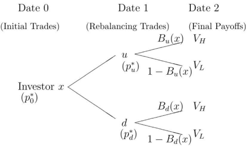
Figure 2. Opinion, Information Structure and Trading Periods
Investors trade in margin at date 0 with their different prior opinion. At date 1, investors learn from the realized state variable as up (u) or down (d), and trade with rebalancing to
satisfy the margin requirement. A final payoff is realized at date 2.
Date 0 Date 1 Date 2
(Initial Trades) (Rebalancing Trades) (Final Payoffs)
Investor x (p∗0) u d (p∗u) (p∗d) Bu(x) 1−Bu(x) 1−Bd(x) Bd(x) VH VL VL VH 28
Table 1: The Impact of Margin Requirement on Stock Prices with Unanticipated Shocks
This illustration considers the set of parameters as VL = 0, VH = 20, W0 = 20, belief structure
B0(x) = 0.25 + 0.5x, u=d= 0.25, and maintenance marginmT = 0.5·m0. The following table
present the results for the effects of margin requirements on the equilibrium.
Table 1: The Impact of Margin Requirements on Stock Prices
This illustration considers the set of parameters as VL = 0, VH = 20, W0 = 20, opinion structure B0(x) = 0.25 + 0.5x, u= d= 0.25, and maintenance margin mT = 0.5·m0. The following table present the results for the effects of margin requirements on the equilibrium. In Table 1 we observe that equilibrium prices are negatively associated with the margin requirement m, and so is the price volatility p∗u−p∗u. This result can be compared to the literature on speculation and volatility.
m0 x∗0 p∗0 xu∗ p∗u x∗d p∗d Fu Fd p∗u−Fu Fd−p∗d p∗u−p∗d 0.30 0.804 13.043 0.886 18.862 0.535 5.351 18.043 8.043 0.819 2.692 13.511 0.35 0.777 12.766 0.859 18.588 0.536 5.359 17.766 7.766 0.822 2.407 13.229 0.40 0.750 12.500 0.831 18.306 0.536 5.357 17.500 7.500 0.806 2.143 12.949 0.45 0.724 12.245 0.802 18.020 0.535 5.348 17.245 7.245 0.775 1.897 12.672 0.50 0.700 12.000 0.773 17.733 0.533 5.333 17.000 7.000 0.733 1.667 12.400 0.55 0.676 11.765 0.745 17.445 0.531 5.313 16.765 6.765 0.681 1.452 12.132 0.60 0.654 11.538 0.716 17.159 0.529 5.288 16.538 6.538 0.620 1.250 11.870 0.65 0.632 11.321 0.687 16.875 0.526 5.260 16.321 6.321 0.554 1.061 11.614 0.70 0.611 11.111 0.659 16.593 0.611 6.111 16.111 6.111 0.482 0.000 10.482 0.75 0.591 10.909 0.632 16.316 0.591 5.909 15.909 5.909 0.407 0.000 10.407 0.80 0.571 10.714 0.604 16.043 0.571 5.714 15.714 5.714 0.329 0.000 10.329 0.85 0.553 10.526 0.577 15.774 0.553 5.526 15.526 5.526 0.248 0.000 10.248 0.90 0.534 10.345 0.551 15.511 0.534 5.345 15.345 5.345 0.166 0.000 10.166 0.95 0.517 10.169 0.525 15.253 0.517 5.169 15.169 5.169 0.083 0.000 10.083 1.00 0.500 10.000 0.500 15.000 0.500 5.000 15.000 5.000 0.000 0.000 10.000 30
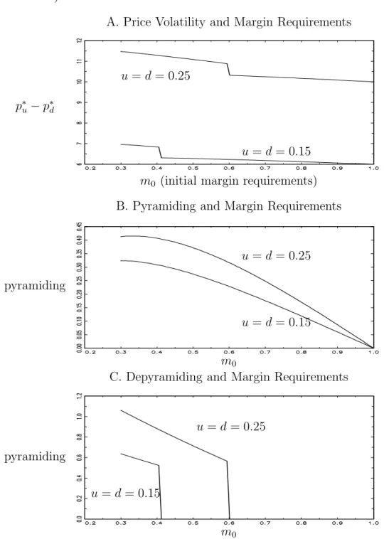
Figure 3: Margin Requirements and Price Volatility, Pyramiding and Depyramding
The following three figures illustrate the impacts of margin requirements on price volatility (p∗u−p∗d), pyramiding (p∗u−Fu(x∗0)) and depyramiding (Fd(x∗0)−p∗d), given the paramenters VH = 20, VL = 0,W0 = 20, B0(x) = 0.25 + 0.5·x, and maintenance margin mT = 0.5·m0. The price volatility, pyramiding and depyramidig are negatively associated with margin requirements, and are all greater in the case with greater shock in investors’ expectations (u=d= 0.25).
A. Price Volatility and Margin Requirements
m0 (initial margin requirements) p∗u−p∗d
u=d= 0.25
u=d= 0.15
B. Pyramiding and Margin Requirements
m0 pyramiding
u=d= 0.25
u=d= 0.15
C. Depyramiding and Margin Requirements
m0 pyramiding
u=d= 0.25
u=d= 0.15
Figure 4: Disperion of Opinion and Price Volatility, Pyramiding and Depyramding
The following three figures illustrate the impacts of dispersion of opinion on price volatility (p∗u−p∗d), pyramiding (p∗u−Fu(x∗0)) and depyramiding (Fd(x∗0)−p∗d), given the paramenters VH = 20, VL= 0, W0 = 20,B0(x) = 0.25 +b·x, u= 0.2,d = 0.25, and maintenance margin mT = 0.5·m0. Generally the price volatility, pyramiding and depyramidig are positively associated with disperion of opinions, except the case when the depyramiding move from positive to zero.
A. Price Volatility and dispersion of opinion
b (dispersion of opinion) p∗u−p∗d
m= 0.5
m = 0.8
B. Pyramiding and and dispersion of opinion
b pyramiding
m = 0.5
m = 0.8
C. Depyramiding and and dispersion of opinion
b pyramiding
m= 0.5
m = 0.8
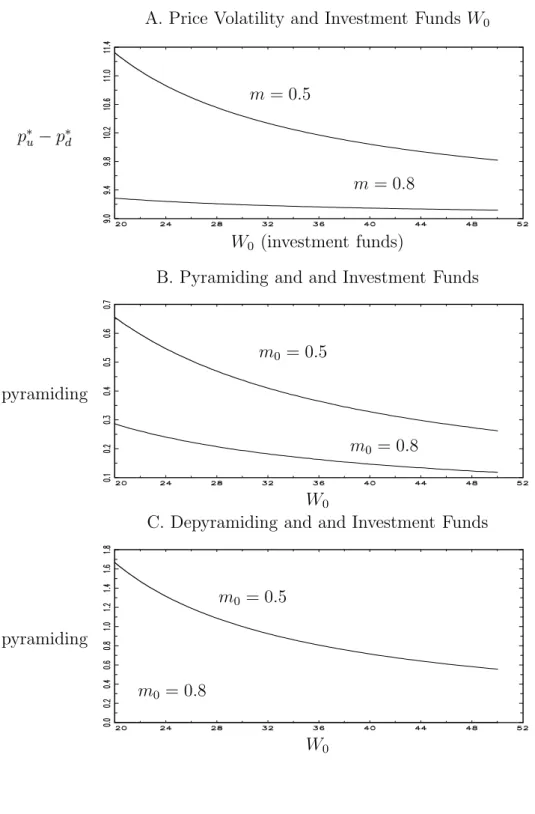
Figure 5: Investment Funds and Price Volatility, Pyramiding and Depyramding
The following three figures illustrate the impacts of margin requirements on price volatility (p∗u−p∗d), pyramiding (p∗u−Fu(x∗0)) and depyramiding (Fd(x∗0)−p∗d), given the paramenters VH = 20, VL = 0, B0(x) = 0.25 + 0.5· x, u = 0.2, d = 0.25, and maintenance margin mT = 0.5·m0. The price volatility, pyramiding and depyramidig are in general negatively associated with investment funds. In Figure C, dypyramiding is 0 when m0 = 0.8.
A. Price Volatility and Investment Funds W0
W0 (investment funds) p∗u−p∗d
m = 0.5
m = 0.8
B. Pyramiding and and Investment Funds
W0 pyramiding
m0 = 0.5
m0 = 0.8
C. Depyramiding and and Investment Funds
W0 pyramiding
m0 = 0.5
m0 = 0.8
Figure 6: The first derivative of expected wealth to the demand when xd< xu.
x
( )
0 E w x D ∂ ⎡⎣ ⎤⎦ ∂( )
1 0 E P −Px
xd
xu
x
011
0
Case III
x
02( )
0 E w x D ∂ ⎡⎣ ⎤⎦ ∂xd
xu
x
01
0
Figure 7: The first derivative of expected wealth to the demand when xu < xd.
x
( )
0 E w x D ∂ ⎡⎣ ⎤⎦ ∂( )
1 0 E P −Px
xd
xu
x
011
0
Case III
x
02( )
0 E w x D ∂ ⎡⎣ ⎤⎦ ∂xd
xu
x
01
0
Table 2: The Impact of Margin Requirement on Price Level and Volatility with Anticipated Shocks.
The following table presents the effects of margin requirements on the equilibrium with anticipated shocks under the set of parameters: a = u = d = 0.1, b = 0.4, VH = 10, W0 =
1, mT = 0.8m0. m0 xu xd x0 Pu Pd P0 Pu−Pd 20% 0.4459 0.4899 0.5666 3.7834 1.9595 2.8328 1.8239 25% 0.4259 0.3716 0.5615 3.7038 1.4864 2.2458 2.2174 30% 0.4084 0.3051 0.5759 3.6336 1.2205 1.9197 2.4131 35% 0.3919 0.2618 0.5979 3.5677 1.0472 1.7084 2.5204 40% 0.3747 0.2313 0.6236 3.4988 0.9253 1.5589 2.5735 45% 0.3558 0.2087 0.6510 3.4232 0.8349 1.4466 2.5883 50% 0.3348 0.1914 0.6792 3.3392 0.7656 1.3585 2.5736 55% 0.3115 0.1777 0.7077 3.2461 0.7109 1.2868 2.5352 60% 0.2860 0.1667 0.7361 3.1439 0.6669 1.2269 2.4769 65% 0.2582 0.1578 0.7641 3.0330 0.6310 1.1755 2.4019 70% 0.2286 0.1504 0.7914 2.9142 0.6014 1.1306 2.3128 75% 0.1972 0.1442 0.8179 2.7888 0.5768 1.0906 2.2120 80% 0.1645 0.1391 0.8434 2.6580 0.5562 1.0543 2.1018
Table 2: The Impact of Margin Requirement on Price Level and Volatility with Anticipated shock.
Following table presents the effects of margin requirements on the equilibrium with antici-pated shock under the set of parameters: a = u = d = 0.1, b = 0.4, VH = 10, W0 = 1, mT =
0.8m0.
Appendix A. Equilibrium with
P
d<
E(
P
1)
< P
0< P
uNow for the most pessimistic investorsx <min{xd, xu}, E
˜ W(x)=W0+D0(x) E(P1)−P0 ,
which is decreasing in D0, thus they hold zero position and are inactive in the stock market.
Since at x = xd, ∂E[ ˜w(x)]/∂D0 takes its maximum, so at equilibria, ∂E[ ˜w(x)]/∂D0
x=xd
must be positive, otherwise all investors don’t hold any stock att= 0, contradicting the market clearing condition.
We can show by contradiction that whenPd<E(P1)< P0 < Pu,xumust be smaller thanxd.
And there are probably two kinds of equilibrium. In the first kind of the equilibrium, investors type x∈(x0,1) buy the stock at t= 0, which is shown in Figure Case 2-1. And conditions for
such equilibrium are:
1. (1−x0)mW0P00 = 1 : market clearing condition att= 0.
2. (1−xd)
W0+ mW0P00(Pd−P0)
m0Pd
= 1 : market clearing condition at the down state. 3. (1−xu)mW0P0u+ (1−x0)mW0P00(Pmu0−PPu0) = 1 : market clearing condition at the up state.
4. E(P1)−P0+θPmu−0PPu0bVH(x0−xu) = 0. 5. ∂E[ ˜W(x)]/∂D0 x=1>0, and∂E[ ˜W(x)]/∂D0 x=xd >0.
x
dx
ux
01
0
x
( )
0 E w x D ∂ ⎡⎣ ⎤⎦ ∂( )
1 0 E P −PCase 2-1
x
dx
ux
011
x
( )
0 E w x D ∂ ⎡⎣ ⎤⎦ ∂( )
1 0 E P −![Figure 1: Social Opinion Structure {B(x)} x∈[0,1] and Marginal Investors A. An Example of B 0 (x)](https://thumb-us.123doks.com/thumbv2/123dok_us/10896.3001038/28.892.222.720.232.565/figure-social-opinion-structure-b-marginal-investors-example.webp)