Claremont Colleges
Scholarship @ Claremont
CMC Faculty Publications and Research
CMC Faculty Scholarship
7-2-2014
Linear Convergence of Stochastic Iterative Greedy
Algorithms with Sparse Constraints
Nam Nguyen
Deanna Needell
Claremont McKenna CollegeTina Woolf
This Article - preprint is brought to you for free and open access by the CMC Faculty Scholarship at Scholarship @ Claremont. It has been accepted for inclusion in CMC Faculty Publications and Research by an authorized administrator of Scholarship @ Claremont. For more information, please [email protected].
Recommended Citation
Nguyen, N., Needell, D., Woolf, T., "Linear Convergence of Stochastic Iterative Greedy Algorithms with Sparse Constraints", Submitted, arXiv preprint arXiv:1407.0088, 2014.
arXiv:1407.0088v1 [math.NA] 1 Jul 2014
Linear Convergence of Stochastic Iterative Greedy Algorithms with
Sparse Constraints
Nam Nguyen, Deanna Needell and Tina Woolf July 2, 2014
Abstract
Motivated by recent work on stochastic gradient descent methods, we develop two stochastic variants of greedy algorithms for possibly non-convex optimization problems with sparsity con-straints. We prove linear convergence1in expectation to the solution within a specified tolerance.
This generalized framework applies to problems such as sparse signal recovery in compressed sensing, low-rank matrix recovery, and covariance matrix estimation, giving methods with prov-able convergence guarantees that often outperform their deterministic counterparts. We also analyze the settings where gradients and projections can only be computed approximately, and prove the methods are robust to these approximations. We include many numerical experi-ments which align with the theoretical analysis and demonstrate these improveexperi-ments in several different settings.
1
Introduction
Over the last decade, the problem of high-dimensional data inference from limited observations has received significant consideration, with many applications arising from signal processing, com-puter vision, and machine learning. In these problems, it is not unusual that the data often lies in hundreds of thousands or even million dimensional spaces while the number of collected sam-ples is sufficiently smaller. Exploiting the fact that data arising in real world applications often has very low intrinsic complexity and dimensionality, such as sparsity and low-rank structure, re-cently developed statistical models have been shown to perform accurate estimation and inference. These models often require solving the following optimization with the constraint that the model parameter is sparse:
min
w F(w) subject to kwk0 ≤k. (1)
Here, F(w) is the objective function that measures the model discrepancy, kwk0 is the ℓ0-norm
that counts the number of non-zero elements of w, and kis a parameter that controls the sparsity of w.
In this paper, we study a more unified optimization that can be applied to a broader class of sparse models. First, we define a more general notion of sparsity. Given the set D ={d1, d2, ...}
consisting of vectors or matricesdi, which we call atoms, we say that the model parameter is sparse
if it can be described as a combination of only a few elements from the atomic set D. Specifically, let w∈Rn be represented as w= k X i=1 αidi, di∈ D, (2) 1
where αi are called coefficients of w; then, w is called sparse with respect to D if k is relatively
small compared to the ambient dimensionn. Here,Dcould be a finite set (e.g. D={ei}ni=1 where ei’s are basic vectors in Euclidean space), or Dcould be infinite (e.g. D={uivi∗}∞i=1 where uivi∗’s
are unit-norm rank-one matrices). This notion is general enough to handle many important sparse models such as group sparsity and low rankness (see [12], [33] for some examples).
Our focus in this paper is to develop algorithms for the following optimization: min w 1 M M X i=1 fi(w) | {z } F(w) subject to kwk0,D ≤k, (3)
where fi(w)’s, w ∈Rn, are smooth functions which can be non-convex; kwk0,D is defined as the
norm that captures the sparsity level of w. In particular, kwk0,D is the smallest number of atoms
inD such thatw can be represented by them: kwk0,D= mink {k:w=
X
i∈T
αidi with |T|=k}. (4)
Also in (3),k is a user-defined parameter that controls the sparsity of the model. The formulation (3) arises in many signal processing and machine learning problems, for instance, compressed sensing (e.g. [16], [8]), Lasso ([39]), sparse logistic regression, and sparse graphical model estimation (e.g. [41]). In the following, we provide some examples to demonstrate the generality of the optimization (3).
1) Compressed sensing: The goal is to recover a signal w⋆ from the set of observations y i =
hai, w⋆i+ǫi for i = 1, ..., m. Assuming that the unknown signal w⋆ is sparse, we minimize the
following to recover w⋆: min w∈Rn 1 m m X i=1 (yi− hai, wi)2 subject to kwk0 ≤k.
In this problem, the setDconsists ofnbasic vectors, each of sizenin Euclidean space. This problem can be seen as a special case of (3) with fi(w) = (yi− hai, wi)2 andM =m. An alternative way to
write the above objective function is 1 m m X i=1 (yi− hai, wi)2 = 1 M M X j=1 1 b jb X i=(j−1)b+1 (yi− hai, wi)2 ,
where M =m/b. Thus, we can treat each function fj(w) as fj(w) = 1bPjbi=(j−1)b+1(yi− hai, wi)2.
In this setting, each fj(w) accounts for a collection (orblock) of observations of sizeb, rather than
only one observation. This setting will be useful later for our proposed stochastic algorithms. 2) Matrix recovery: Givenmobservationsyi =hAi, W⋆i+ǫi fori= 1, .., mwhere the unknown
matrix W⋆ ∈Rd1×d2 is assumed low-rank, we need to recover the original matrix W⋆. To do so,
we perform the following minimization: min W∈Rd1×d2 1 m m X i=1 (yi− hAi, Wi)2 subject to rank(W)≤k.
In this problem, the set D consists of infinitely many unit-normed rank-one matrices and the functionsfi(W) = (yi−hAi, Wi)2. We can also write functions in the block formfi(W) = 1bP(yi−
3) Covariance matrix estimation: Letx be a Gaussian random vector of sizenwith covariance matrix W⋆. The goal is to estimate W⋆ from m independent copies x
1, ..., xm of x. A useful way
to findW⋆ is via solving the maximum log-likelihood function with respect to a sparse constraint
on the precision matrix Σ⋆ = (W⋆)−1. The sparsity of Σ⋆ encourages the independence between
entries of x. The minimization formula is as follows: min Σ 1 m m X i=1 xixTi ,Σ
−log det Σ subject to kΣoffk0≤k,
where Σoff is the matrix Σ with diagonal elements set to zero. In this problem, D is the finite
collection of unit-normedn×nmatrices{eie∗j}and the functionsfi(Σ) =xixTi ,Σ
−m1 log det Σ.
Our paper is organized as follows. In the remainder of Section1 we discuss related work in the literature and highlight our contributions; we also describe notations used throughout the paper and assumptions employed to analyze the algorithms. We present our stochastic algorithms in Sections 2 and 3, where we theoretically show the linear convergence rate of the algorithms and include a detailed discussion. In Section 4, we explore various extensions of the two proposed algorithms and also provide the theoretical result regarding the convergence rate. We apply our main theoretical results in Section 5, in the context of sparse linear regression and low-rank matrix recovery. In Section 6, we demonstrate several numerical simulations to validate the efficiency of the proposed methods and compare them with existing deterministic algorithms. Our conclusions are given in Section7. We reserve Section 8for our theoretical analysis.
1.1 Related work and our contribution
Sparse estimation has a long history and during its development there have been many great ideas along with efficient algorithms to solve (not exactly) the optimization problem (3). We sketch here some main lines which are by no means exhaustive.
Convex relaxation. Optimization based techniques arose as a natural convex relaxation to the problem of sparse recovery (3). There is now a massive amount of work in the field of Compressive Sensing and statistics [7,13] that demonstrates these methods can accurately recover sparse signals from a small number of noisy linear measurements. Given noisy measurements y =Aw⋆ +e, one
can solve theℓ1-minimization problem
ˆ
w= argmin
w k
wk1 such that kAw−yk2 ≤ε,
where ε is an upper bound on the noise kek2 ≤ ε. Cand`es, Romberg and Tao [11, 9] prove that
under a deterministic condition on the matrixA, this method accurately recovers the signal, kw⋆−wˆk2 ≤ε+k
w⋆−w⋆
kk2
√
k , (5)
wherew⋆k denotes thek largest entries in magnitude of the signal w⋆. The deterministic condition is called the Restricted Isometry Property (RIP) [11] and requires that the matrixA behave nicely on sparse vectors:
(1−δ)kxk22≤ kAxk22 ≤(1 +δ)kxk22 for allk-sparse vectors x,
for some small enoughδ <1.
The convex approach is also extended beyond the quadratic objectives. In particular, the convex relaxation of the optimization (3) is the following:
min
where the regularization kwk is used to promote sparsity, for instance, it can be the ℓ1 norm
(vector case) or the nuclear norm (matrix case). Many methods have been developed to solve these problems including interior point methods and other first-order iterative methods such as (proximal) gradient descent and coordinate gradient descent (e.g. [27,18,14]). The theoretical analyses of these algorithms have also been studied with either linear or sublinear rate of convergence, depending on the assumption imposed on the functionF(w). In particular, sublinear convergence rate is obtained if F(w) exhibits a convex and smooth function, whereas the linear convergence rate is achieved whenF(w) is the smooth and strongly convex function. For problems such as compressed sensing, although the loss function F(w) does not possess the strong convexity property, experiments still show the linear convergence behavior of the gradient descent method. In the recent work [1], the authors develop theory to explain this behavior. They prove that as long as the function F(w) obeys the restricted strong convexity and restricted smoothness, a property similar to the RIP, then gradient descent algorithm can obtain the linear rate.
Greedy pursuits. More in line with our work are greedy approaches. These algorithms re-construct the signal by identifying elements of the support iteratively. Once an accurate support set is located, a simple least-squares problem recovers the signal accurately. Greedy algorithms like Orthogonal Matching Pursuit (OMP) [40] and Regularized OMP (ROMP) [30] offer a much faster runtime than the convex relaxation approaches but lack comparable strong recovery guaran-tees. Recent work on greedy methods like Compressive Sampling Matching Pursuit (CoSaMP) and Iterative Hard Thresholding (IHT) offer both the advantage of a fast runtime and essentially the same recovery guarantees as (5) (e.g. [29,5, 45,19]). However, these algorithms are only applied for problems in compressed sensing where the least square loss is used to measure the discrepancy. There certainly exists many loss functions that are commonly used in statistical machine learning and do not exhibit quadratic structure such as log-likelihood loss. Therefore, it is necessary to develop efficient algorithms to solve (3).
There are several methods proposed to solve special instances of (3). [36] and [35] propose the forward selection method for sparse vector and low-rank matrix recovery. The method selects each nonzero entry or each rank-one matrix in an iterative fashion. [43] generalizes this algorithm to the more general dictionary D. [44] proposes the forward-backward method in which an atom can be added or removed from the set, depending on how much it contributes to decrease the loss function. [25] extends this algorithms beyond the quadratic loss studied in [44]. [3] extends the CoSaMP algorithm for a more general loss function. Very recently, [33] further generalizes CoSaMP and proposes the Gradient Matching Pursuit (GradMP) algorithm to solve (3). This is perhaps the first greedy algorithm for (3) - the very general form of sparse recovery. They show that under a restricted convexity assumption of the objective function, the algorithm linearly converges to the optimal solution. This desirable property is also possessed by CoSaMP. We note that there are other algorithms having also been extended to the setting of sparsity in arbitrary D but only limited to the quadratic loss setting, see e.g. [15,20,21,22].
We outline the GradMP method here, since it will be used as motivation for the work we propose. GradMP [33] is a generalization of the CoSaMP [29] that solves a wider class of sparse reconstruction problems. Like OMP, these methods consist of four main steps: i) form a signal proxy, ii) select a set of large entries of the proxy, iii) use those as the support estimation and estimate the signal via least-squares, and iv) prune the estimation and repeat. Methods like OMP and CoSaMP use the proxy A∗(y−Awt); more general methods like GradMP use the gradient
∇F(wt) (see [33] for details). The analysis of GradMP depends on the restricted strong convexity
and restricted strong smoothness properties as in Definitions 1 and 2 below, the first of which is motivated by a similar property introduced in [31]. Under these assumptions, the authors prove linear convergence to the noise floor.
The IHT, another algorithm that motivates our work, is a simple method that begins with an estimation w0 = 0 and computes the next estimation using the recursion
wt+1 =H
k(wt+A∗(y−Awt)),
whereHk is the thresholding operator that sets all but the largest (in magnitude) kcoefficients of
its argument to zero. Blumensath and Davies [5] prove that under the RIP, IHT provides a recovery bound comparable to (5). [24] extends IHT to the matrix recovery. Very recently, [42] proposes the Gradient Hard Thresholding Pursuit (GraHTP), an extension of IHT to solve a special vector case of (3).
Stochastic convex optimization. Methods for stochastic convex optimization have been developed in a very related but somewhat independent large body of work. We discuss only a few here which motivated our work, and refer the reader to e.g. [37, 6] for a more complete survey. Stochastic Gradient Descent (SGD) aims to minimize a convex objective function using unbiased stochastic gradient estimates, typically of the form∇fi(w) whereiis chosen stochastically. For the
optimization (3) with no constraint, this can be summarized concisely by the update rule
wt+1 =wt−α∇fi(wt),
for some step size α. For smooth objective functions F(w), classical results demonstrate a 1/t
convergence rate with respect to the objective difference F(wt)−F(w⋆). In the strongly convex
case, Bach and Moulines [2] improve this convergence to a linear rate, depending on the average squared condition number of the system. Recently, Needell et. al. draw on connections to the Kaczmarz method (see [26, 38] and references therein), and improve this to a linear dependence on the uniform condition number [28]. Another line of work is the Stochastic Coordinate Descent (SCD) beginning with the work of [32]. Extension to minimization of composite functions in (6) is described in [34].
Contribution. In this paper, we exploit ideas from IHT [5], CoSaMP [29] and GradMP [33] as well as the recent results in stochastic optimization [38,28], and propose two new algorithms to solve (3). The IHT and CoSaMP algorithms have been remarkably popular in the signal processing community due to their simplicity and computational efficiency in recovering sparse signals from incomplete linear measurements. However, these algorithms are mostly used to solve problems in which the objective function is quadratic and it would be beneficial to extend the algorithmic ideas to the more general objective function.
We propose in this paper stochastic versions of the IHT and GradMP algorithms, which we term Stochastic IHT (StoIHT) and Stochastic GradMP (StoGradMP). These algorithms possess favorable properties toward large scale problems:
• The algorithms do not need to compute the full gradient ofF(w). Instead, at each iteration, they only sample one index i ∈ [M] ={1,2, ..., M} and compute its associated gradient of
fi(w). This property is particularly efficient in large scale settings in which the gradient
computation is often prohibitively expensive.
• The algorithms do not need to perform an optimal projection at each iteration as required by the IHT and CoSaMP. Approximated projection is generally sufficient to guarantee linear convergence while the algorithms enjoy significant computational improvement.
• Under the restricted strong convexity assumption of F(w) and the restricted strong smooth-ness assumption of fi(w) (defined below), the two proposed algorithms are guaranteed to
• The algorithms and proofs can be extended further to consider other variants such as inexact gradient computations and inexact estimation.
1.2 Notations and assumptions
Notation: For a set Ω, let |Ω| denote its cardinality and Ωc denote its complement. We will
write D as the matrix whose columns consist of elements ofD, and denoteDΩ as the submatrix
obtained by extracting the columns of Dcorresponding to the indices in Ω. We denote by R(DΩ)
the space spanned by columns of the matrix DΩ. Also denote by PΩw the orthogonal projection
of w onto R(DΩ). Given a vector w ∈ Rn that can decomposed as w = Pi∈Ωαidi, we say that
the support of w with respect to D is Ω, denoted by suppD(w) = Ω. We denote by [M] the set
{1,2, ..., M}. We also define Ei as the expectation with respect to i where i is drawn randomly
from the set [M]. For a matrix A, we use conventional notations: kAk and kAkF are the spectral
norm and Frobenius norms of the matrix A. For the linear operator A:W ∈Rn1×n2 →y ∈ Rm,
A∗ :y∈Rm →W ∈Rn1×n2 is the transpose of A.
Denote F(w), M1 PMi=1fi(w) and let p(1), ..., p(M) be the probability distribution of an index
iselected at random from the set [M]. Note thatPMi=1p(i) = 1. Another important observation is that if we select an indexifrom the set [M] with probability p(i), then
Ei
1
M p(i)fi(w) =F(w) and Ei
1
M p(i)∇fi(w) =∇F(w), (7)
where the expectation is with respect to the index i.
Define approxk(w, η) as the operator that constructs a set Γ of cardinality ksuch that
kPΓw−wk2 ≤ηkw−wkk2, (8)
where wk is the bestk-sparse approximation of w with respect to the dictionaryD, that is, wk=
argminy∈DΓ,|Γ|≤kkw−yk2. Put another way, denote Γ∗= argmin
|Γ|≤k k
w− PΓwk2.
Then, we require that
kw− PΓwk2≤ηkw− PΓ∗wk
2. (9)
An immediate consequence is the following inequality:
kw− PΓwk2 ≤ηkw− PRwk2. (10)
for any set of |R| ≤k atoms ofD. This follows because kw− PΓ∗wk
2≤ kw− PRwk2. In addition,
taking the square on both sides of the above inequality and manipulating yields kPRwk22≤ 1 η2 kPΓwk 2 2+ η2−1 η2 kwk 2 2 =kPΓwk 2 2+ η2−1 η2 kPΓcwk 2 2.
Taking the square root gives us an important inequality for our analysis later. For any set of|R| ≤k
atoms of D,
kPRwk2≤ kPΓwk2+
s
η2−1
Assumptions: Before describing the two algorithms in the next section, we provide assumptions for the functions fi(w) as well as F(w). The first assumption requires that F(w) is restricted
strongly convex with respect to the setD. Although we do not requireF(w) to be globally convex, it is necessary thatF(w) is convex in certain directions to guarantees the linear convergence of our proposed algorithms. The intuition is that our greedy algorithms only drive along certain directions and seek for the optimal solution. Thus, a global convexity assumption is not necessary.
Definition 1 (D-restricted strong convexity (D-RSC)). The functionF(w) satisfies the D-RSC if there exists a positive constant ρ−k such that
F(w′)−F(w)−∇F(w), w′ −w≥ ρ − k 2 w′−w22, (12)
for all vectors w andw′ of size nsuch that |suppD(w)∪suppD(w′)| ≤k.
We notice that the left-hand side of the above inequality relates to the Hessian matrix ofF(w) (provided F(w) is smooth) and the assumption essentially implies the positive definiteness of the
k×k Hessian submatrices. We emphasize that this assumption is much weaker than the strong convexity assumption imposed on the fullndimensional space where the latter assumption implies the positive definiteness of the full Hessian matrix. In fact, when k=n,F(w) exhibits a strongly convex function with parameterρ−k, and whenρ−k = 0,F(w) is a convex function. We also highlight that theD-RSC assumption is particularly relevant when studying statistical estimation problems in the high-dimensional setting. In this setting, the number of observations is often much less than the dimension of the model parameter and therefore, the Hessian matrix of the loss functionF(w) used to measure the data fidelity is highly ill-posed.
In addition, we require that fi(w) satisfies the so-called D-restricted strong smoothness which is
defined as follows:
Definition 2 (D-restricted strong smoothness (D-RSS)). The function fi(w) satisfies the D-RSS
if there exists a positive constant ρ+k(i) such that
∇fi(w′)− ∇fi(w)
2≤ρ+k(i)w′−w2 (13) for all vectors w andw′ of size nsuch that |suppD(w)∪suppD(w′)| ≤k.
Variants of these two assumptions have been used to study the convergence of the projected gradient descent algorithm [1]. In fact, the names restricted strong convexity and restricted strong smoothness are adopted from [1].
In this paper, we assume that the functions fi(w) satisfy D-RSS with constants ρ+k(i) for all
i = 1, ..., M and F(w) satisfies D-RSC with constant ρ−k. The following quantities will be used
extensively throughout the paper:
αk,max i ρ+k(i) M p(i), ρ + k ,maxi ρ+k(i), and ρ+k , 1 M M X i=1 ρ+k(i). (14)
2
Stochastic Iterative Hard Thresholding (StoIHT)
In this section, we describe the Stochastic Iterative Hard Thresholding (StoIHT) algorithm to solve (3). The algorithm is provided in Algorithm 1. At each iteration, the algorithm performs the following standard steps:
• Select an indexifrom the set [M] with probability p(i).
• Compute the gradient associated with the index just selected and move the solution along the gradient direction.
• Project the solution onto the constraint space via the approx operator defined in (8).
Ideally, we would like to compute the exact projection onto the constraint space or equivalently the best k-sparse approximation of bt with respect to D. However, the exact projection is often
hard to evaluate or is computationally expensive in many problems. Take an example of the large scale matrix recovery problem, where computing the best matrix approximation would require an intensive Singular Value Decomposition (SVD) which often costs O(kmn), where m and n are the matrix dimensions. On the other hand, recent linear algebraic advances allow computing an approximate SVD in onlyO(k2max{m, n}). Thus, approximate projections could have a significant computational gain in each iteration. Of course, the price paid for fast approximate projections is a slower convergence rate. In Theorem1 we will show this trade-off.
Algorithm 1 StoIHT algorithm
input: k,γ,η,p(i), and stopping criterion
initialize: w0 and t= 0
repeat
randomize: select an indexit from [M] with probability p(it)
proxy: bt=wt− γ M p(it)∇fit(w t) identify: Γt= approx k(bt, η) estimate: wt+1=P Γt(bt) t=t+ 1
until halting criterion true
output: wˆ=wt
Denote w⋆ as a feasible solution of (3). Our main result provides the convergence rate of the
StoIHT algorithm via characterizing the ℓ2-norm error of t-th iterate wt with respect to w⋆. We
first define some quantities necessary for a precise statement of the theorem. First, we denote the contraction coefficient κ,2 q 1−γ(2−γα3k)ρ−3k+ q (η2−1) 1 +γ2α 3kρ+3k−2γρ−3k, (15)
where the quantities α3k, ρ+3k,ρ−3k and η are defined in (14), (12), and (8). As will become clear
later, the contraction coefficientκcontrols the algorithm’s rate of convergence and is required to be less than unity. Thisκis intuitively dependent on the characteristics of the objective function (via D-RSC and D-RSS constantsρ+3k andρ−3k), the user-defined step size, the probability distribution, and the approximation error. The price paid for allowing a larger approximation errorηis a slower convergence rate, since κ will also become large; however, η should not be allowed too large since
κ must still be less than one.
We also define the tolerance parameter
σw⋆, γ miniM p(i) 2Ei max |Ω|≤3kkPΩ∇fi(w ⋆) k2+ p η2−1Eik∇fi(w⋆) k2 , (16)
where i is an index selected from [M] with probability p(i). Of course when w⋆ minimizes all
components fi, we have σw⋆ = 0, and otherwise σw⋆ measures (a modified version) of the usual
In terms of these two ingredients, we now state our first main result. The proof is deferred to Section8.2.
Theorem 1. Let w⋆ be a feasible solution of (3) and w0 be the initial solution. At the (t+ 1)-th
iteration of Algorithm 1, the expectation of the recovery error is bounded by
Ewt+1−w⋆2 ≤κt+1w0−w⋆2+ σw⋆
(1−κ) (17)
where σw⋆ is defined by (16),κ is defined by (15) and is assumed to be strictly less than unity, and
expectation is taken over all choices of random variables i0, ..., it.
The theorem demonstrates a linear convergence for the StoIHT even though the full gradient computation is not available. This is a significant computational advantage in large-scale settings where computing the full gradient often requires performing matrix multiplications with matrix dimensions in the millions. In addition, a stochastic approach may also gain advantages from parallel implementation. We emphasize that the result of Theorem1holds for any feasible solution
w⋆ and the error of the (t+ 1)-th iterate is mainly governed by the second term involving the
gradient of{fi(w⋆)}i=1,...,M. For certain optimization problems, we expect that the energy of these
gradients associated with the global optimum is small. For statistical estimation problems, the gradient of the true model parameter often involves only the statistical noise, which is small. Thus, after a sufficient number of iterations, the error between wt+1 and the true statistical parameter is
only controlled by the model noise.
The result is significantly simpler when the optimal projection is available at each iteration. That is, the algorithm is always able to find the set Γtsuch thatwt+1 is the bestk-sparse
approx-imation of bt. In this case,η = 1 and the contraction coefficientκ in (15) is simplified to
κ= 2 q 1−γ(2−γα3k)ρ−3k, with α3k = maxi ρ + 3k(i) M p(i) and σw⋆ = 2γ miniM p(i)Eimax|Ω|≤3kkPΩ∇fi(w ⋆)k 2. In order for κ < 1, we needρ−3k≥ 34α3k= 34maxi ρ+3k(i) M p(i) and γ < 1 +q1−3α3k 4ρ− 3k α3k .
The following corollary provides an interesting particular choice of the parameters in which Theorem1 is easier to access.
Corollary 1. Suppose that ρ−3k ≥ 34ρ+3k. Select γ = α13k, η = 1 and the probability distribution
p(i) = M1 for all i= 1, ..., M. Then using the quantities defined by (14),
Ewt+1−w⋆2 ≤κt+1w0−w⋆2+ 2γ (1−κ) miniM p(i)E i max |Ω|≤3kkPΩ∇fi(w ⋆) k2, where κ= 2 r 1−ρ − 3k ρ+3k.
When the exact projection is not available, we would want to see how big η is such that the StoIHT still allows linear convergence. It is clear from (15) that for a given step size γ, bigger η
leads to biggerκ, or slower convergence rate. It is required by the algorithm thatκ <1. Therefore,
η2 must at least satisfy
η2≤1 + 1 1 +γ2α 3kρ+3k−2γρ−3k . (18) As γ = 1 ρ+3k and p(i) = 1
M, i= 1, ..., M, the bound is simplified toη2 ≤1 +
1 2(1−ρ−
3k)
. This bound implies that the approximation error in (9) should be at most (1+ǫ) away from the exact projection error whereǫ∈(0,1).
In Algorithm 1, the projection tolerance η is fixed during the iterations. However, there is a flexibility in changing it every iteration. The advantage of this flexibility is that this parameter can be set small during the first few iterations where the convergence is slow and gradually increased for the later iterations. Denoting the projection tolerance at thej-th iteration by ηj, we define the
contraction coefficient at the j-th iteration:
κj ,2 q 1−γ(2−γα3k)ρ−3k +q((ηj)2−1) 1 +γ2α 3kρ+3k−2γρ−3k , (19)
and thetolerance parameter σw⋆ ,maxj∈[t]σjw⋆ where
σwj⋆ , γ miniM p(i) 2Ei max |Ω|≤3kkPΩ∇fi(w ⋆) k2+ q (ηj)2−1 max i Eik∇fi(w ⋆) k2 . (20)
The following corollary shows the convergence of the StoIHT algorithm in the case where the projection tolerance is allowed to vary at each iteration:
Corollary 2. At the (t+ 1)-th iteration of Algorithm 1, the recovery error is bounded by
Ewt+1−w⋆2 ≤w0−w⋆2 t+1 Y j=0 κj +σw⋆ t X i=0 t Y j=t−i κj, (21)
where κj is defined by (19), andσw⋆ = maxj
∈[t]σwj⋆ is defined via (20).
3
Stochastic Gradient Matching Pursuit (StoGradMP)
CoSaMP [29] has been a very popular algorithm to recover a sparse signal from its linear mea-surements. In [33], the authors generalize the idea of CoSaMP and provide the GradMP algorithm that solves a broader class of sparsity-constrained problems. In this paper, we develop a stochastic version of the GradMP, namely StoGradMP, in which at each iteration only the evaluation of the gradient of a functionfi is required. The StoGradMP algorithm is described in Algorithm2 which
consists of following steps at each iteration:
• Randomly select an indexiwith probability p(i). • Compute the gradient of fi(w) with associated index i.
• Choose the subspace of dimension at most 2k to which the gradient vector is closest, then merge with the estimated subspace from previous iteration.
• Solve a sub-optimization problem with the search restricted on this subspace.
• Find the subspace of dimension k which is closest to the solution just found. This is the estimated subspace which is hopefully close to the true subspace.
At a high level, StoGradMP can be interpreted as at each iteration, the algorithm looks for a subspace based on the previous estimate and then seeks a new solution via solving a low-dimensional sub-optimization problem. Due to theD-RSC assumption, the sub-optimization is convex and thus it can be efficiently solved by many off-the-shelf algorithms. StoGradMP stops when a halting criterion is satisfied.
Algorithm 2 StoGradMP algorithm
input: k,η1,η2,p(i), and stopping criterion
initialize: w0, Λ = 0, andt= 0
repeat
randomize: select an indexit from [M] with probability p(it)
proxy: rt=∇f it(w t) identify: Γ = approx2k(rt, η 1) merge: bΓ = Γ∪Λ estimate: bt= argmin wF(w) w∈span(DbΓ) prune: Λ = approxk(bt, η 2) update: wt+1=P Λ(bt) t = t+1
until halting criterion true
output: wˆ=wt
Denote w⋆ as a feasible solution of the optimization (3). We will present our main result for the StoGradMP algorithm. As before, our result controls the convergence rate of the recovery error at each iteration. We define thecontraction coefficient
κ,(1 +η2) rα 4k ρ−4k max i p M p(i) v u u t2 η2 1−1 η2 1 ρ + 4k−ρ−4k ρ−4k + p η2 1 −1 η1 , (22)
where the quantitiesα4k,ρ+4k,ρ−4k,η1, andη2 are defined in (14), (12), and (8). As will be provided
in the following theorem, κ characterizes the convergence rate of the algorithm. This quantity depends on many parameters that play a role in the algorithm.
In addition, we define analogously as before thetolerance parameter
σw⋆ ,C(1 +η2) 1 mini∈[M]M p(i) max |Ω|≤4k,i∈[M]kPΩ∇fi(w ⋆)k 2, (23) whereC is defined as C, 1 ρ− 4k 2 maxi∈[M]M p(i) qα4 k ρ− 4k + 3 .
We are now ready to state our result for the StoGradMP algorithm. The error bound has the same structure as that of StoIHT but with a different convergence rate.
Theorem 2. Let w⋆ be a feasible solution of (3) and w0 be the initial solution. At the (t+ 1)-th
iteration of Algorithm 2, the recovery error is bounded by
Ewt+1−w⋆2≤κt+1w0−w⋆2+ σw⋆
1−κ (24)
where σw⋆ is defined by (23),κ is defined by (22) and is assumed to be strictly less than unity, and
When p(i) = M1 ,i= 1, ..., M, andη1 =η2 = 1 (exact projections are obtained), the contraction
coefficient κ has a very simple representation: κ = 2 r ρ+4k ρ− 4k ρ+ 4k ρ− 4k −
1. This expression of κ is the same as that of the GradMP. In this situation, the requirement κ < 1 leads to the condition
ρ+4k< 2+4√6ρ−4k. The following corollary provides the explicit form of the recovery error.
Corollary 3. Using the parameters described by (14), suppose that ρ−4k > 4 2+√6ρ
+
4k. Select η1 =
η2 = 1, and the probability distribution p(i) = M1 , i= 1, ..., M. Then,
Ewt+1−w⋆2≤ 2 s ρ+4k(ρ+4k−ρ−4k) (ρ−4k)2 !t+1 w0−w⋆2+σw⋆, where σw⋆ = 2 ρ− 4k 2 r ρ+ 4k ρ− 4k + 3 max|Ω|≤4k,i∈[M]kPΩ∇fi(w⋆)k2.
Similar to the StoIHT, the theorem demonstrates the linear convergence of the StoGradMP to the feasible solution w⋆. The expected recovery error naturally consists of two components:
one relates to the convergence rate and the other concerns the tolerance factor. As long as the contraction coefficient is small (less than unity), the first component is negligible, whereas the second component can be very large depending on the feasible solution we measure. We expect that the gradients of fi’s associated with the global optimum to be small, as shown true in many
statistical estimation problems such as sparse linear estimation and low-rank matrix recovery, so that the StoGradMP converges linearly to the optimum. We note that the linear rate here is precisely consistent with the linear rate of the original CoSaMP algorithm applied to compressed sensing problems [29]. Furthermore, StoGradMP gains significant computation over CoSaMP and GradMP since the full gradient evaluation is not required at each iteration.
In Algorithm 2, the parametersη1 andη2 are fixed during the iterations. However, they can be
changed at each iteration. Denoting the projection tolerances at the j-th iteration by η1j and η2j, we define the contraction coefficient at thej-th iteration as
κj ,(1 +η2j) rα 4k ρ−4k maxi p M p(i) v u u u t 2(η1j)2 −1 (ηj1)2 ρ+4k−ρ−4k ρ−4k + q (η1j)2−1 ηj1 . (25)
Also define thetolerance parameter σw⋆ ,maxj∈[t]σjw⋆ where
σwj⋆ ,C(1 +η j 2) 1 mini∈[M]M p(i) max |Ω|≤4k,i∈[M]kPΩ∇fi(w ⋆)k 2 (26)
andC is defined asC,2 maxi∈[M]M p(i)qα4k
ρ−
4k
+ 3. The following corollary shows the convergence of the algorithm.
Corollary 4. At the (t+ 1)-th iteration of Algorithm 2, the recovery error is bounded by
Ewt+1−w⋆2 ≤w0−w⋆2 t+1 Y j=0 κj +σw⋆ t X i=0 t Y j=t−i κj, (27)
4
StoIHT and StoGradMP with inexact gradients
In this section, we investigate the StoIHT and StoGradMP algorithms in which the gradient might not be exactly estimated. This issue occurs in many practical problems such as distributed network optimization in which gradients are corrupted by noise during the communication on the network. In particular, in both algorithms, the gradient selected at each iteration is contaminated by a noise vector et where t indicates the iteration number. We assume {et}
t=1,2,... are deterministic noise
with bounded energies.
4.1 StoIHT with inexact gradients
In the StoIHT algorithm, the update bt at the proxy step has to take into account the noise
appearing in the gradient. In particular, at the t-th iteration,
bt=wt− γ
M p(it) ∇
fit(w
t) +et.
Denote the quantity
σe, γ miniM p(i) max j∈[t] 2 max |Ω|≤3k PΩej2+pη2−1ej 2 . (28)
We state our result in the following theorem. The proof is deferred to Section 8.4.
Theorem 3. Let w⋆ be a feasible solution of (3). At the (t+ 1)-th iteration of Algorithm 1 with
inexact gradients, the expectation of the recovery error is bounded by
Ewt+1−w⋆ 2≤κ t+1w0−w⋆ 2+ 1 (1−κ)(σw⋆+σe), (29) where κ is defined in (15) and is assumed to be strictly less than unity and expectation is taken over all choices of random variables i1, ..., it. The quantities σw⋆ and σe are defined in (16) and
(28), respectively.
Theorem3provides the linear convergence of StoIHT even in the setting of an inexact gradient computation. The error bound shares a similar structure as that of the StoIHT with only an additional term related to the gradient noise. An interesting property is that the noise does not accumulate over iterations. Rather, it only depends on the largest noise level.
4.2 StoGradMP with inexact gradients
In the StoGradMP algorithm, accounting for noise in the gradient appears in the proxy step; the expression of rt, with an additional noise term, becomes
rt=∇fit(w
t) +et.
Denote the quantity
σe, maxip(i) ρ−4kminip(i) max j∈[t] ej2. (30)
Theorem 4. Let w⋆ be a feasible solution of (3). At the (t+ 1)-th iteration of Algorithm 2 with
inexact gradients, the expectation of the recovery error is bounded by
Ewt+1−w⋆2≤κt+1w0−w⋆2+ 1
(1−κ)(σw⋆+σe), (31) where κ is defined in (22) and is assumed to be strictly less than unity and expectation is taken over all choices of random variables i1, ..., it. The quantities σw⋆ and σe are defined in (23) and
(30), respectively.
Similar to the StoIHT, StoGradMP is stable under the contamination of gradient noise. Stability means that the algorithm is still able to obtain the linear convergence rate. The gradient noise only affects the tolerance rate and not the contraction factor. Furthermore, the recovery error only depends on the largest gradient noise level, implying that the noise does not accumulate over iterations.
4.3 StoGradMP with inexact gradients and approximated estimation
In this section, we extend the theory of the StoGradMP algorithm further to consider the sub-optimality of optimization at the estimation step. Specifically, we assume that at each iteration, the algorithm only obtains an approximated solution of the sub-optimization. Denote
btopt= argmin
w
F(w) subject to w∈span(DbΓ), (32) as the optimal solution of this convex optimization, where ˆΓ = Γ∪Λ may also give rise to an approximation at the identification step. Write bt as the approximated solution available at the
estimation step. Thenbtis linked tobt
opt via the relationship:
bt−bt opt 2 ≤ǫ t. This consideration
is realistic in two aspects: first, the optimization (32) can be too slow to converge to the optimal solution, hence we might want to stop the algorithm after a sufficient number of steps or whenever the solution is close to the optimum; second, even if (32) has a closed-form solution as the least-squares problem, it is still beneficial to solve it approximately in order to reduce the computational complexity caused by the pseudo-inverse process (see [17] for an example of randomized least-squares approximation). Denoting the quantity
σǫ = max j∈[t]ǫ
j, (33)
we have the following theorem.
Theorem 5. Let w⋆ be a feasible solution of (3). At the (t+ 1)-th iteration of Algorithm 2 with inexact gradients and approximated estimations, the expectation of the recovery error is bounded by
Ewt+1−w⋆2 ≤κt+1w0−w⋆2+ 1
(1−κ)(σw⋆+σe+σǫ), (34) where κ is defined in (22) and is assumed to be strictly less than unity and expectation is taken over all choices of random variables i1, ..., it. The quantities σw⋆, σe, and σǫ are defined in (23),
(30), and (33), respectively.
Theorem5shows the stability of StoGradMP under both the contamination of gradient noise at the proxy step and the approximate optimization at the estimation step. Furthermore, StoGradMP still achieves a linear convergence rate even in the presence of these two sources of noise. Similar to the artifacts of gradient noise, the approximated estimation affects the tolerance rate and not the contraction factor, and the recovery is only impacted by the largest approximated estimation bound (rather than an accumulation over all of the iterations).
5
Some estimates
In this section we investigate some specific problems which require solving an optimization with a sparse constraint and transfer results of Theorems1 and2.
5.1 Sparse linear regression
The first problem of interest is the well-studied sparse recovery in which the goal is to recover a
k0-sparse vector w0 from noisy observations of the following form:
y=Aw0+ξ.
Here, the m×n matrixA is called the design matrix and ξ is them dimensional vector noise. A natural way to recover w0 from the observation vector y is via solving
min w∈Rn 1 2mky−Awk 2 2 subject to kwk0 ≤k, (35)
where k is the user-defined parameter which is assumed greater than k0. Clearly, this
opti-mization is a special form of (3) with D being the collection of standard vectors in Rn and
F(w) = 21mky−Awk22. Decompose the vector y into non-overlapping vectors ybi of size b and
denote Abi as the bi×nsubmatrix of A. We can then rewrite F(w) as
F(w) = 1 M M X i=1 1 2bkybi−Abiwk 2 2 , 1 M M X i=1 fi(w),
where M =m/b. In order to apply Theorems 1 and 2 for this problem, we need to compute the contraction coefficient and tolerance parameter which involve the D-RSC and D-RSS conditions. It is easy to see that these two properties ofF(w) and{fi(w)}Mi=1 are equivalent to the RIP studied
in [9]. In particular, we require that the matrix A satisfies 1
mkAwk
2
2 ≥(1−δk)kwk22
for all k-sparse vectorsw. In addition, the matricesAbi,i= 1, ..., M, are also required to obey
1
bkAbiwk
2
2≤(1 +δk)kwk22
for all k-sparse vectors w. Here, (1 +δk) and (1−δk) with δk ∈(0,1] play the role of ρ+k(i) and
ρ−k in Definitions 1and 2, respectively. For the Gaussian matrix A (entries are i.i.d. N(0,1)), it is well-known that these two assumptions hold as long asm≥ Ckδlogn
k and b≥
cklogn
δk . By setting the
block sizeb=cklogn, the number of blocks M is thus proportional to klogmn.
Now using StoIHT to solve (35) and applying Theorem 1, we set the step size γ = 1, the approximation error η = 1, and p(i) = 1/M, i = 1, ..., M, for simplicity. Thus, the quantities in (14) are all the same and equal to 1 +δk. It is easy to verify that the contraction coefficient
defined in (15) is κ = 2q2δ3k−δ23k. One can obtain κ ≤ 3/4 when δ3k ≤ 0.07, for example. In
addition, since w0 is the feasible solution of (35), the tolerance parameter σw0 defined in (16) can
be rewritten as σw0 = 2Ei max |Ω|≤3k 1 b PΩA∗biξbi 2 ≤ 2 b √ 3kmax i∈[M]maxj∈[n]| hAbi,j, ξbii |,
whereAbi,j is thej-th column of the matrixAbi. For stochastic noiseξ∼ N(0, σ 2I m), it is easy to verify that σw0 ≤c′ q σ2klogn
b with probability at least 1−n−1.
Using StoGradMP to solve (35) with the same setting as above, we write the contraction coefficient in (22) as κ = 2q2δ4k(1+δ4k)
(1−δ4k)2 , which is less than 3/4 if δ4k ≤ 0.05. The tolerance
parameter σw0 in (23) can be simplified similarly as in StoIHT. We now provide the following
corollary based on what we have discussed.
Corollary 5 (for StoIHT and StoGradMP). Assume A ∈Rm×n satisfies the D-RSC and D-RSS assumptions and ξ ∼ N(0, σ2). Then with probability at least 1−n−1, the error at the (t+ 1)-th iterate of the StoIHT and StoGradMP algorithms is bounded by
Ewt+1−w02 ≤(3/4)t+1kw0k2+c
r
σ2k
0logn
b .
We describe the convergence result of the two algorithms in one corollary since their results share the same form with the only difference in the constant c. One can see that for a sufficient number of iterations, the first term involvingkw0k2is negligible and the recovery error only depends
on the second term. When the noise is absent, both algorithms guarantee recovery of the exactw0.
The recovery error also depends on the block size b. When b is small, more error is expected, and the error decreases as b increases. This of course matches our intuition. We emphasize that the deterministic IHT and GradMP algorithms deliver the same recovery error with breplaced by m.
5.2 Low-rank matrix recovery
We consider the high-dimensional matrix recovery problem in which the observation model has the form
yj =hAj, W0i+ξj , j = 1, ..., m,
whereW0 is then1×n2 unknown rank-k0 matrix, each measurement Aj is anm×n1 matrix, and
the noise ξj is assumed N(0, σ2). Noting that 21mPmj=1(yj − hAj, Wi)2 = 21mky− A(W)k22, the
standard approach to recover W0 is to solve the minimization
min W∈Rn1×n2 1 2mky− A(W)k 2 2 subject to rank(W)≤k, (36)
withkassumed greater thank0. Here, Ais the linear operator. In this problem, the setDconsists
of infinitely many unit-normed rank-one matrices and the objective function can be written as a summation of sub-functions: F(W) = 1 M M X i=1 fi(W) = 1 M M X i=1 1 2b ib X j=(i−1)b+1 (yj− hAj, Wi)2 , 1 M M X i=1 1 2bkybi − Ai(W)k 2 2,
wherem=M b(assumebis integer). Eachfi(W) accounts for a collection (or block) of observations
ybi of size b. In this case, theD-RSC andD-RSS properties are equivalent to the matrix-RIP [10],
which holds for a wide class of random operators A. In particular, we require 1
mkA(W)k
2
2 ≥(1−δk)kWk2F
for all rank-k matrices W. In addition, the linear operators Ai are required to obey
1
bkAi(W)k
2
for all rank-k matrices W. Here, (1 +δk) and (1−δk) with δk ∈(0,1] play the role of ρ+k(i) and
ρ−k in Definitions 1 and 2, respectively. For the random Gaussian linear operator A (vectors Ai
are i.i.d. N(0, I)), it is well-known that these two assumptions hold as long as m ≥ Ck(n1+n2)
δk
and b ≥ ck(n1+n2)
δk . By setting the block size b = ck(n1 +n2), the number of blocks M is thus
proportional to k(nm
1+n2).
In this section, we consider applying results of Theorems3and5. To do so, we need to compute the contraction coefficients and tolerance parameter. We begin with Theorem 3, which holds for the StoIHT algorithm. Similar to the previous section,κin (15) can have a similar form. However, in the matrix recovery problem, SVD computations are required at each iteration which is often computationally expensive. There has been a vast amount of research focusing on approximation methods that perform nearly as good as exact SVD but with much faster computation. Among them are the randomized SVD [23] that we will employ in the experimental section. For simplicity, we set the step sizeγ = 1 andp(i) = 1/M for alli. Thus, quantities in (14) are the same and equal to 1 +δk. Rewriting κ in (15), we have κ= 2 q 2δ3k−δ23k+ q (η2−1)(δ2 3k+ 4δ3k),
where we recall η is the projection error. Setting κ ≤ 3/4 by allowing the first term to be less than 1/2 and the second term less than 1/4, we obtain δ4k ≤0.03 and the approximation error η
is allowed up to 1.19.
The next step is to evaluate the tolerance parameter σW0 in (16). The parameter σW0 can be
read as σW0 = 2Ei max |Ω|≤4k 1 b kPΩA∗i(ξbi)kF + p η2−1Ei1 b kA∗i(ξbi)kF ≤ 2 b √ 4kmax i kA ∗ i(ξbi)k+ 1 b p η2−1√nmax i kA ∗ i(ξbi)k.
For stochastic noise ξ ∼ N(0, σ2I), it is shown in [10], Lemma 1.1 thatkA∗i(ξbi)k ≤ c
√
σ2nb with
probability at least 1−n−1 wheren= max{n1, n2}. Therefore,σW0 ≤c
q σ2kn b + q (η2 −1)σ2n2 b . In addition, the parameter σe in (28) is estimated as
σe ≤max j 2 max |Ω|≤3k PΩEjF +pη2−1Ej F ≤max j 2√3kEj+pη2−1Ej F ,
where we recall thatEjis the noise matrix that might contaminate the gradient at thej-th iteration.
Applying Theorem3 leads to the following corollary.
Corollary 6 (for StoIHT). Assume the linear operator Asatisfies the D-RSC andD-RSS assump-tions and ξ ∼ N(0, σ2). Set p(i) = 1/M for i= 1, ..., M and γ = 1. Then with probability at least
1−n−1, the error at the(t+ 1)-th iterate of the StoIHT algorithm is bounded by
EWt+1−W0 F ≤(3/4)t+1kW0kF +c r σ2kn b + r (η2−1)σ2n2 b ! + 4 max j∈[t] 2√3kEj+pη2−1Ej F .
The discussion after Corollary5for the vector recovery can also be applied here. For a sufficient number of iterations, the recovery error is naturally controlled by three factors: the measurement noise σ, the approximation projection parameter η, and the largest gradient noise Ej. In the
absence of these three parameters, the recovery is exact. When η= 1 and Ej = 0, j= 0, ..., t, the
error has the same structure as the convex nuclear norm minimization method [10] which has been shown to be optimal.
Moving to the StoGradMP algorithm, setting p(i) = 1/M fori= 1, ..., M again for simplicity, we can write the contraction coefficient in (22) as
κ= (1 +η2) s 1 +δ4k 1−δ4k v u u t2η 2 1−1 η2 1 (1 +δ4k)−(1−δ4k) 1−δ4k + p η21−1 η1 .
If we allow for example the projection error η1 = 1.01 and η2 = 1.01 and requireκ ≤0.9, simple
algebra gives usδ4k≤0.03 In addition, for stochastic noiseξ∼ N(0, σ2I), the tolerance parameter
σW0 in (23) can be read as σW0 =c(1 +η2) max i∈[M],|Ω|≤4kkPΩA ∗ i(ξbi)kF ≤c1(1 +η2) √ 4kmax i∈[M]kA ∗ i(ξbi)k ≤c2(1 +η2) r σkn b
with probability at least 1−n−1. Again, the last inequality is due to [10]. Now applying Theorem
5, where we recall the parameter σe in (30) is σe= maxj
Ej
F andǫ
j is the optimization error at
the estimation step, we have the following corollary.
Corollary 7 (for StoGradMP). Assume the linear operator A satisfies the D-RSC and D-RSS assumptions and ξ ∼ N(0, σ2). Set p(i) = 1/M for i = 1, ..., M. Then with probability at least 1−n−1, the error at the(t+ 1)-th iterate of the StoGradMP algorithm is bounded by
EWt+1−W0 F ≤(0.9)t+1kW0kF +c(1 +η2) r σ2kn b + 4 maxj∈[t] EjF + 4 max j∈[t]ǫ j.
6
Numerical experiments
In this section we present some experimental results comparing our proposed stochastic methods to their deterministic counterparts. Our goal is to explore several interesting aspects of improvements and trade-offs; we have not attempted to optimize algorithm parameters. Unless otherwise speci-fied, all experiments are run with at least 50 trials, “exact recovery” is obtained when the signal recovery error kw−wˆk2 drops below 10−6, and the plots illustrate the 10% trimmed mean. For
the approximation error versus epoch (or iteration) plots, the trimmed mean is calculated at each epoch (or iteration) value by excluding the highest and lowest 5% of the error values (rounding when necessary). For the approximation error versus CPU time plots, the trimmed mean compu-tation is the same, except the CPU time values corresponding to the excluded error values are also excluded from the mean CPU time. We begin with experiments in the compressed sensing setting, and follow with application to the low-rank matrix recovery problem.
6.1 Sparse vector recovery
The first setting we explored is standard compressed sensing which has been studied in Subsection
standard Gaussian. The signal is measured with anm×256 i.i.d. standard Gaussian measurement matrix. First, we compare signal recovery as a function of the number of measurements used, for various sparsity levels s. Each algorithm terminates upon convergence or upon a maximum of 500 epochs2. We used a block size of b= min(s, m) for sparsity level k0 and number of measurements m, except when k0 = 4 and m > 5 we used b = 8 in order to obtain consistent convergence.
Specifically, this means that bmeasurements were used to form the signal proxy at each iteration of the stochastic algorithms. For the IHT and StoIHT algorithms, we use a step size ofγ = 1. The results for IHT and StoIHT are shown in Figure 1and GradMP and StoGradMP in Figure2. Here we see that with these parameters, StoIHT requires far fewer measurements than IHT to recover the signal, whereas GradMP and StoGradMP are comparable.
0 50 100 150 200 250 0 20 40 60 80 100 Number of Measurements m
Percentage of Signals Recovered (%) 00 50 100 150 200 250
20 40 60 80 100 Number of Measurements m
Percentage of Signals Recovered (%)
s = 4 s = 8 s = 12 s = 20 s = 28 s = 36
Figure 1: Sparse Vector Recovery: Percent recovery as a function of the number of measurements for IHT (left) and StoIHT (right) for various sparsity levels k0.
0 50 100 150 200 250 0 20 40 60 80 100 Number of Measurements m
Percentage of Signals Recovered (%) 00 50 100 150 200 250
20 40 60 80 100 Number of Measurements m
Percentage of Signals Recovered (%)
s = 4 s = 8 s = 12 s = 20 s = 28 s = 36
Figure 2: Sparse Vector Recovery: Percent recovery as a function of the number of measurements for GradMP (left) and StoGradMP (right) for various sparsity levelsk0.
Next we explore how the choice of block size affects performance. We employ the same setup as described above, only now we fix the number of measurements m (m= 180 for the IHT methods
2
We refer to an epoch as the number of iterations needed to use m rows. Thus for deterministic non-blocked methods, an epoch is one iteration, whereas for a method using blocks of sizeb, an epoch ism/biterations.
and m = 80 for the GradMP methods), allow a maximum of 100 epochs, and use various block sizes in the stochastic algorithms. The sparsity of the signal is k0 = 8. The results are depicted
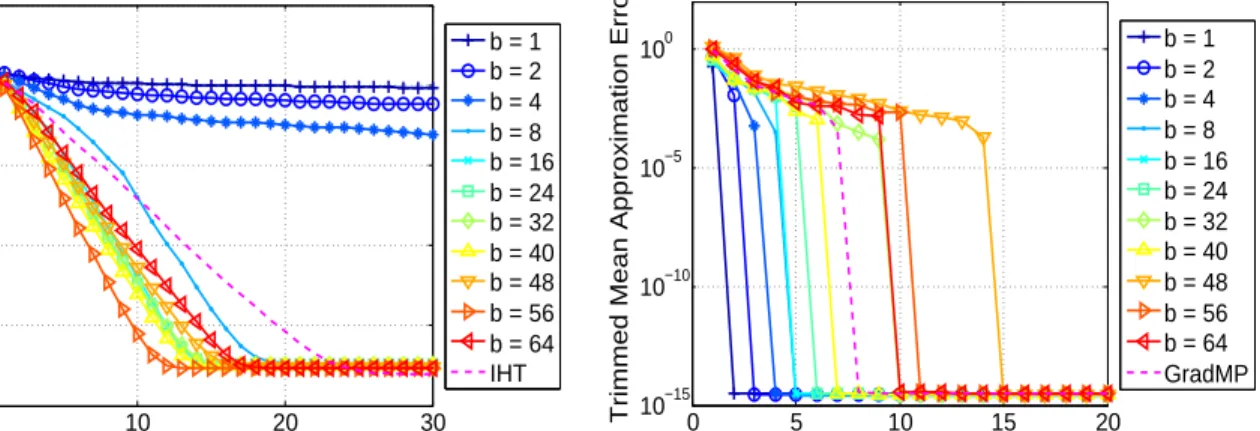
for both methods in Figure 3. Here we see that in both cases, the deterministic methods seem to offer intermediate performance, outperforming some block sizes and underperforming others. It is interesting that the StoIHT method seems to prefer larger block sizes whereas the StoGradMP seems to prefer smaller sizes. This is likely because StoGradMP, even using only a few gradients may still estimate the support accurately, and thus the signal accurately.
0 10 20 30 10−8 10−6 10−4 10−2 100 102 Epoch
Trimmed Mean Approximation Error
b = 1 b = 2 b = 4 b = 8 b = 16 b = 24 b = 32 b = 40 b = 48 b = 56 b = 64 IHT 0 5 10 15 20 10−15 10−10 10−5 100 Epoch
Trimmed Mean Approximation Error
b = 1 b = 2 b = 4 b = 8 b = 16 b = 24 b = 32 b = 40 b = 48 b = 56 b = 64 GradMP
Figure 3: Sparse Vector Recovery: Recovery error as a function of epochs and various block sizes
bfor HT methods (left) and GradMP methods (right).
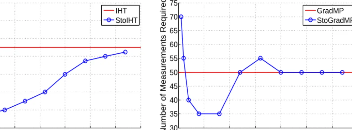
Next we repeat the same experiments but examine the recovery error as a function of the number of measurements for various block sizes (note that if the block size exceeds the number of measurements, we simply use the entire matrix as one block). Figure4shows these results. Because the methods exhibit graceful decrease in recovery error, here we plot the number of measurements (as a function of block size) required in order for the estimation error kw−wˆk2 to drop and
remain below 10−6. Although block size is not a parameter for the deterministic methods IHT and
GradMP, a red horizontal line at the number of measurements required is included for comparison. We see that the fewest measurements are required when the block sizes are about 10 (recall the signal dimension is 256). We also note that StoIHT requires fewer measurements than IHT for large blocks, whereas StoGradMP requires the same as GradMP for large blocks, which is not surprising. However, we see that both methods offer improvements over their deterministic counterparts if the block sizes are chosen correctly.
6.2 Robustness to measurement noise
We next repeat the above sparse vector recovery experiments in the presence of noise in the mea-surements. All experiment parameters remain as in the previous setup, but a vector eof Gaussian noise with kek2 = 0.5 is added to the measurement vector. We again compare the recovery error
against the number of epochs and measurements needed. The results are shown in Figures 5 and
6 for the IHT and GradMP algorithms, respectively. The right hand plots show the number of measurements required for the error to drop below the noise level 0.5 as a function of block size. Overall, the methods are robust to noise and demonstrate the same improvements and heuristics as in the noiseless experiments.
0 10 20 30 40 50 60 70 60 80 100 120 140 160 180 200 Block Size
Number of Measurements Required
IHT StoIHT 0 10 20 30 40 50 60 70 30 35 40 45 50 55 60 65 70 75 Block Size
Number of Measurements Required
GradMP StoGradMP
Figure 4: Sparse Vector Recovery: Number of measurements required for signal recovery as a func-tion of block size (blue marker) for StoIHT (left) and StoGradMP (right). Number of measurements required for deterministic method shown as red solid line.
0 20 40 60 80 100
10−1 100
Epoch
Trimmed Mean Approximation Error
b = 1 b = 2 b = 4 b = 8 b = 16 b = 24 b = 32 b = 40 b = 48 b = 56 b = 64 IHT 0 10 20 30 40 50 60 70 60 80 100 120 140 160 180 200 Block Size
Number of Measurements Required
IHT StoIHT
Figure 5: Sparse Vector Recovery: A comparison of IHT and StoIHT in the presence of noise. Recovery error versus epoch (left) and measurements required versus block size (right).
6.3 The choice of step size in StoIHT
Our last experiment in the sparse vector recovery setting explores the role of the step size γ in StoIHT. Keeping the dimension of the signal at 256, the sparsity k0 = 8, the number of
measure-ments m= 80, no noise, and fixing the block size b= 8, we test the algorithm using various values of the step size γ. The results are shown in Figure 7. We see that the value of γ clearly plays a role, but the range of successful values is quite large. Not surprisingly, too small of a step size leads to extremely slow convergence, and too large of one leads to divergence (at least initially).
6.4 Low-Rank Matrix Recovery
We now turn to the setting where we wish to recover a low-rank matrix W0 from m linear
mea-surements as studied in Subsection 5.2. Here W0 is the 10×10 matrix with rank k0 and we take m linear Gaussian measurements of the form yi = hAi, W0i, where each Ai is a 10×10 matrix
0 10 20 30 10−0.6
10−0.5 10−0.4
Epoch
Trimmed Mean Approximation Error
b = 1 b = 2 b = 4 b = 8 b = 16 b = 24 b = 32 b = 40 b = 48 b = 56 b = 64 GradMP 0 10 20 30 40 50 60 70 40 45 50 55 60 65 70 75 80 Block Size
Number of Measurements Required
GradMP StoGradMP
Figure 6: Sparse Vector Recovery: A comparison of GradMP and StoGradMP in the presence of noise. Recovery error versus epoch (left) and measurements required versus block size (right). (where again we deem the signal is recovered exactly when the error kW0 −WˆkF is below 10−6)
against the number of measurements required, for various rank levels. For the matrix case, we use a step size of γ = 0.5 for both the IHT and StoIHT methods, which seems to work well in this setting. The results for IHT and StoIHT are shown in Figure8and for GradMP and StoGradMP in Figure9. For this choice of parameters, we see that both StoIHT and StoGradMP tend to require fewer measurements to recover the signal.
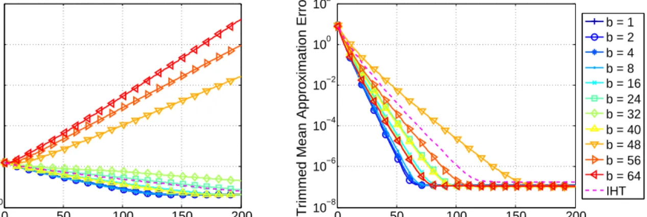
Next we examine the signal recovery error as a function of epoch, for various block sizes and against the deterministic methods. We fix the rank to be k0 = 2 in these experiments. Because
both block size and number of measurements affect the convergence, we see different behavior in the low measurement regime and the high measurement regime. This is apparent in Figure 10, where
m= 90 measurements are used in the plot on the left andm = 140 measurements are used in the plot on the right, which shows the convergence of the IHT methods per epoch for various block sizes. We again see that for proper choices of block sizes, the StoIHT method outperforms IHT. It is also interesting to note that IHT seems to reach a higher noise floor than StoIHT. Of course we again point out that we have not optimized any of the algorithm parameters for either method. Results for the GradMP methods are shown in Figure 11, again where m = 90 measurements are used in the plot on the left and m= 140 measurements are used in the plot on the right. Similar to the IHT results, proper choices of block sizes allows StoGradMP to require much fewer epochs than GradMP to achieve convergence.
Figure 12 compares the block size and the number of measurements required for exact signal recovery for the IHT methods and the GradMP methods, again for a fixed rank of k0 = 2. We
again see that StoIHT and StoGradMP prefer small block sizes.
6.5 Recovery with approximations
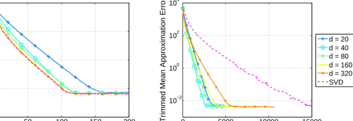
Finally, we consider the important case where the identification, estimation, and pruning steps can only be performed approximately. In particular, we consider the case of low-rank matrix recovery in which these steps utilize only an approximate Singular Value Decomposition (SVD) of the matrix. This may be something that is unavoidable in certain applications, or may be desirable in others for computational speedup. For our first experiments of this kind, we use N = 1024 and generate a N ×N rank k0 = 40 matrix. We take m permuted rows of the N ×N discrete
0 500 1000 1500 2000 10−10 10−5 100 105
Iteration
Trimmed Mean Approximation Error
0.010.03 0.05 0.07 0.09 0.2 0.4 0.6 0.8 1 1.2 1.4 1.6
Figure 7: Sparse Vector Recovery: A comparison of StoIHT for various values of the step size γ
(shown in the colorbar).
40 trials. In the StoIHT experiments we takem = 0.3N2, and in the StoGradMP experiments we takem= 0.35N2; these values formempirically seemed to work well with the two algorithms. For each trial of the approximate SVD, we also run 5 sub-trials, to account for the randomness used in the approximate SVD algorithm. Here we use the randomized method described in [23] to compute the approximate SVD of a matrix. Briefly, to obtain a rank-s approximation of a matrix X and compute its approximated SVD, one applies the matrix to a randomly generatedN×(s+d) matrix Ω to obtain the productY =XΩ and constructs an orthonormal basisQ for the column space of
Y. Here,dis anover-sampling factor that can be tuned to balance the tradeoff between accuracy and computation time. Using this basis, one computes the SVD of the productB =Q∗X=UΣV∗,
and approximates the SVD ofX byX≈(QU)ΣV∗. Because (s+d) is typically much less than N, significant speedup can be gained. In addition, [23] proves that the approximation error is bounded by kX−XskF ≤ 1 + r s s+d X−Xsbest F ,
where Xsbest is the best rank-s approximation of X and Xs is the approximate rank-s matrix
produced from the above procedure. Here, the multiplicative error is associated with the quantity
η in the approximation operator approxs(w, η) defined in (8).
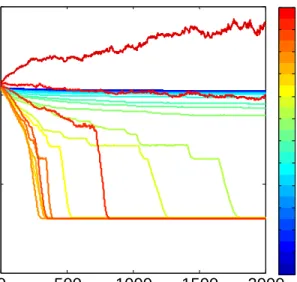
Figure 13 shows the approximation error as a function of epoch and runtime for the StoIHT algorithm, for various over-sampling factorsdas well as the full SVD computation for comparison. We again use a 10% trimmed mean over all the trials, and a step-size ofγ = 0.5. We see that in terms of epochs, for reasonably sized over-sampling factors, the convergence using the SVD approximation is very similar to that of using the full SVD. In terms of runtime, we see a significant speedup for moderate choices of over-sampling factor, as expected. Recall that 2 blocks were used for this experiment, but we have observed a very similar relationship between the curves when increasing the number of blocks to 10.
0 50 100 150 200 0 20 40 60 80 100 Number of Measurements m
Percentage of Signals Recovered (%) 00 50 100 150 200
20 40 60 80 100 Number of Measurements m
Percentage of Signals Recovered (%)
s = 1 s = 2 s = 3 s = 4 s = 5
Figure 8: Low-Rank Matrix Recovery: Percent recovery as a function of the number of measure-ments for IHT (left) and StoIHT (right) for various rank levels s.
0 50 100 150 200 0 20 40 60 80 100 Number of Measurements m
Percentage of Signals Recovered (%) 00 50 100 150 200
20 40 60 80 100 Number of Measurements m
Percentage of Signals Recovered (%)
s = 1 s = 2 s = 3 s = 4 s = 5
Figure 9: Low-Rank Matrix Recovery: Percent recovery as a function of the number of measure-ments for GradMP (left) and StoGradMP (right) for various rank levels k0.
see that for certain over-sampling factors, the convergence of the approximation error as a function of epoch is similar when using the approximate SVD and the full SVD. We also see a very significant speedup when using the approximate SVD; in this case, all the over-sampling factors used in this experiment offer an improved runtime over the full SVD computation.
7
Conclusion
We study in this paper two stochastic algorithms to solve a possibly non-convex optimization prob-lem with the constraint that the solution has a simple representation with respect to a predefined atom set. This type of optimization has found tremendous applications in signal processing, ma-chine learning, and statistics such as sparse signal recovery and low-rank matrix estimation. Our proposed algorithms, called StoIHT and StoGradMP, have their roots back to the celebrated IHT and CoSaMP algorithms, from which we have made several significant extensions. The first exten-sion is to transfer algorithmic ideas of IHT and CoSaMP to the stochastic setting and the second extension is the allowance of approximate projections at each iteration of the algorithms. More