University of New Hampshire
University of New Hampshire Scholars' Repository
Master's Theses and Capstones Student Scholarship
Winter 2016
Interactive Visual Analytics for Large-scale Particle
Simulations
Erol Aygar
University of New Hampshire, Durham
Follow this and additional works at:https://scholars.unh.edu/thesis
This Thesis is brought to you for free and open access by the Student Scholarship at University of New Hampshire Scholars' Repository. It has been accepted for inclusion in Master's Theses and Capstones by an authorized administrator of University of New Hampshire Scholars' Repository. For more information, please [email protected].
Recommended Citation
Aygar, Erol, "Interactive Visual Analytics for Large-scale Particle Simulations" (2016).Master's Theses and Capstones. 896.
INTERACTIVE VISUAL ANALYTICS FOR LARGE-SCALE PARTICLE SIMULATIONS
BY
Erol Aygar
MS, Bosphorus University, 2006 BS, Mimar Sinan Fine Arts University, 1999
THESIS
Submitted to the University of New Hampshire in Partial Fulfillment of
the Requirements for the Degree of
Master of Science in
ALL RIGHTS RESERVED c
2016 Erol Aygar
This thesis has been examined and approved in partial fulfillment of the requirements for the de-gree of Master of Science in Computer Science by:
Thesis Director, Colin Ware Professor of Computer Science University of New Hampshire
R. Daniel Bergeron
Professor of Computer Science University of New Hampshire
Thomas Butkiewicz
Research Assistant Professor of Computer Science University of New Hampshire
On November 2, 2016
Dedication
Acknowledgments
I hereby acknowledge and thank my mentor, Dr. Colin Ware, who supported this research and made it possible. I would like to thank my committee members: Dr. Bergeron and Dr. Butkiewicz for their interest and expertise. I want to thank to my academic advisors, Dr. Michael Jonas, Dr. Michaela Sabin, and Dr. Philip Hatcher who encouraged me throughout my academic journey and helped achieve my goals.
I would also like to thank my colleagues who provided technical and logistical support through-out this research, including Drew Stevens, Roland Arsenault.
Preface
Initial chapter of this thesis consists of an article that has been submitted for publication [Aygar and Ware, 2016, Ware et al., 2016].
Table of Contents
DEDICATION . . . iv ACKNOWLEDGEMENT . . . v PREFACE . . . vi TABLE OF CONTENTS . . . ix LIST OF TABLES . . . x LIST OF FIGURES . . . xi ABSTRACT . . . xii 1 Introduction 1 1.1 Model simulation as a scientific inquiry method . . . 21.2 Workflows . . . 2
1.3 Visualization Pipeline . . . 3
1.4 Data Size . . . 3
1.5 Data Reduction Methods . . . 4
1.5.1 Sampling . . . 4
1.5.2 In-situ . . . 5
1.5.3 An in-situ solution based on images (Cinema) . . . 5
1.5.4 Visualization and Perception . . . 6
1.6 Problem Statement . . . 7
1.7 Approach . . . 8
1.8 Structure of the Work . . . 9
2 Application Domain: Dark Matter in the Universe 10 2.1 Cosmology . . . 10
2.2 The Roadrunner Universe MC3 . . . 11
2.3 Dataset . . . 11
3 Perceptual Consideration 14 3.1 Structure from Motion . . . 15
3.2 Stereoscopic Viewing . . . 16
4 Human Factors Experiments 21 4.1 Experiment 1 . . . 22 4.1.1 Conditions . . . 22 4.1.2 Test Patterns . . . 23 4.1.3 Task . . . 24 4.1.4 Participants . . . 25 4.1.5 Procedure . . . 25 4.1.6 Display/Hardware . . . 26 4.1.7 Results . . . 26 4.2 Experiment 2 . . . 27 4.2.1 Conditions . . . 28 4.2.2 Participants . . . 28
4.2.3 Results from Experiment 2 . . . 28
4.3 Meta-Analysis . . . 29
4.4 Discussion . . . 30
5 The Interactive Interface 33 5.1 Rationale . . . 33
5.1.1 Functional Requirements . . . 34
5.2 Literature Review . . . 35
5.2.1 Interacting with Point Clouds . . . 36
5.2.2 Open Source Toolkits and Libraries . . . 38
5.3 Software Application . . . 42
5.3.1 High Level Design . . . 42
5.3.2 User Interface . . . 42
5.3.3 Navigation . . . 43
5.3.4 Spherical area of interest . . . 44
5.3.5 Motion . . . 45
5.3.6 Stereoscopic viewing . . . 45
5.3.7 Visualization Parameters . . . 46
5.3.8 Tracing particles over time . . . 48
5.4 Implementation . . . 49
5.4.1 Overview . . . 49
5.4.2 Data Management (Spatial Partitioning and Range Search Operations) . . . 52
5.4.3 Approach . . . 53
5.4.5 Development . . . 56 5.4.6 Rendering . . . 56 5.4.7 Rendering into image files . . . 59
6 Conclusion 60
6.1 Summary . . . 60 6.2 Future Work . . . 62
A IRB Approval Form 63
B Participant Consent Form 65
C Supplementary Materials 67
D Manual 68
BIBLOGRAPHY 77
List of Tables
3.1 Effect of motion, stereo and combination . . . 20
4.1 Hypotheses . . . 22
4.2 Parameters used to generate background data . . . 24
5.1 Particle sample size . . . 55
5.2 Frustum Parameters . . . 57
List of Figures
2.1 The Roadrunner Universe MC3 . . . 12
2.2 The Roadrunner Universe MC3 Dataset . . . 12
2.3 Halos data:a single time step with 1.67M particles . . . 13
3.1 Stereoscopic disparity . . . 17
4.1 Oscilation . . . 21
4.2 Artificially generated background . . . 23
4.3 Sample Targets . . . 25
4.4 Experiment 1 Results . . . 27
4.5 Experiment 2 Results . . . 29
4.6 Experiment 1 and 2 Results . . . 30
5.1 Forms of Interaction . . . 39
5.2 User Interface . . . 43
5.3 Spherical Area of Interest . . . 45
5.4 Streamlets . . . 47
5.5 Color . . . 47
5.6 Stremlets . . . 48
5.7 Velocity and directions . . . 49
5.8 The interactive Interface . . . 50
5.9 Variation over time . . . 51
5.10 Spatial Partitioning . . . 53
5.11 Logical Particle Data Structure . . . 54
5.12 Class Diagram . . . 55
5.13 Frustum . . . 58
5.14 Asymmetric Frustum . . . 58
A.1 IRB approval . . . 64
Abstract
INTERACTIVE VISUAL ANALYTICS FOR LARGE-SCALE PARTICLE SIMULATIONS by
Erol Aygar
University of New Hampshire, December, 2016
Particle based model simulations are widely used in scientific visualization. In cosmology, par-ticles are used to simulate the evolution of dark matter in the universe. Clusters of parpar-ticles (that have special statistical properties) are called halos. From a visualization point of view, halos are clusters of particles, each having a position, mass and velocity in three dimensional space, and they can be represented as point clouds that contain various structures of geometric interest such as filaments, membranes, satellite of points, clusters, and cluster of clusters.
The thesis investigates methods for interacting with large scale datasets represented as point clouds. The work mostly aims at the interactive visualization of cosmological simulation based on large particle systems. The study consists of three components: a) two human factors experi-ments into the perceptual factors that make it possible to see features in point clouds; b) the de-sign and implementation of a user interface making it possible to rapidly navigate through and visualize features in the point cloud, c) software development and integration to support visual-ization.
Chapter 1
Introduction
Particle based simulations are used in computational models for a number of scientific applica-tions, including simulations of fluids [M¨uller et al., 2003], to study space weather events [Lapenta, 2012], and to understand the formation of the universe [Habib et al., 2009]. These simulations are powered by high performance computing (HPC) systems. Data generation rates are increasing dramatically with advances in HPC and this is causing problems for visualization applications, and the overall workflow. As a consequence, visual analysis tasks are increasingly performed when data still resides in memory as opposed to after a model run. This method is called in-situ data analysisorin-situ visualization. These advancements also have impact on the nature of products that offer visual analysis solutions.
In cosmology, particles are used to simulate the evolution of dark matter in the universe [Habib et al., 2009]. Clusters of particles (that have special statistical properties) are calledhalos. From a visualization point of view, halos are clusters of particles, each having a position, mass and ve-locity in three dimensional space, and they can be represented as point clouds that contain vari-ous structures of geometric interests, such as filaments, membranes, satellite of points, clusters, and cluster of clusters. This thesis explores methods for interacting with large scale cosmology datasets represented as point clouds.
The following sections of this chapter begin with a basic description of the role of model simu-lations in scientific inquiry and then discuss key concepts that provide background information about applications related to the challenges of visualizing large-scale particle simulations.
Fi-nally, the rationale behind this thesis is presented in more detail.
1.1
Model simulation as a scientific inquiry method
Traditional experimental methods rely on data collected from natural events through observations and measurements. This is followed by analysis of the data to construct theoretical explanations and to draw conclusions about the object of the inquiry [Langley and Stanford, 1995, Schickore, 2014]. With the advent of high performance computing (HPC), the process incorporates mathe-matical models and simulation of the phenomenon in ways that are beyond the reach of experi-ments. Scientists are now able to incorporate datasets from many different sources, such as data captured by instruments, data collected from sensor networks, and data generated by simulations, to cross-validate their outcomes. This is commonly recognized as data-intensive science or com-puting [Hey, 2012, Ahrens et al., 2010]. Because of advances in HPC, scientists are able to sim-ulate nature with higher level of detail, precision and accuracy. Consequently, weather forecasts become more accurate, products and services are designed in a more economical way, and we now can study complex physical and engineering systems in a scale and fidelity which otherwise not possible. Thus, model simulations have become an integral part of the scientific inquiry pro-cess.
1.2
Workflows
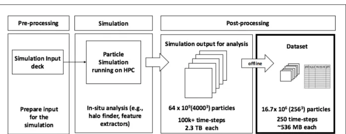
Commonly used visual analysis workflows can be characterized by three main stages: preparing the input (pre-processing), simulation run (execution) and analysis of the data generated by the model (post-processing).
As a part of the post-processing stage, the analysis is performed separately in a computer sys-tem dedicated to the task. During a model run, the data is saved in the form of model dumps (checkpoint-restart files). However, the files generated from model dumps are both extremely
large and not ideal for visual analysis. Due to the size of such data sets, tasks like viewing, edit-ing, or presenting the data have become a challenge, as the data is too large to fit into the memory of the visualization computer. In some cases, the data is even too large to move through the net-work or to store in local storage units. Instead, we need methods for saving model data in ways that are both compact and optimized for visual analysis.
1.3
Visualization Pipeline
One of the most common abstractions used by visual analysis products is what is known as the visualization pipeline. This metaphor provides the key structure in many visualization develop-ment systems and incorporates operations such as transforming, filtering, rendering, and saving the data. The visualization pipeline represents the flow of data in which computation is described as a collection of static constructs (data operations) that are connected in a directed graph. Many current projects involve solutions based on pipeline architecture because of the abundance of ex-isting implementations and the flexibility they offer.
Most of the HPC systems are based on massively threaded, heterogeneous, accelerator-based ar-chitectures. Traditional pipelines are not compatible with this form of computing. Instead, in-situ visualization is done using customized distributed rendering methods.
There are a number of open source efforts to provide visual analysis. Most of these solutions fo-cus on the traditional post processing approach. Moreland et al provided an extensive survey of visualization pipelines and these efforts [Moreland, 2013].
1.4
Data Size
Large-scale scientific simulations typically output time-varying multivariate volumetric data, and current leading edge computers can perform computation power used in simulations is in
petas-cale range. Consequently, HPC based particle simulations generate petabytes of data that simply cannot be handled effectively by traditional methods. The need for new techniques and tools for storing, transferring, accessing, visualizing, and analyzing large datasets is pressing. For exam-ple, a commonly recognized simulation system dedicated to astrophysics and cosmology sim-ulations runs petascale range (1015floating point operations per second) which generates 64 x
109particles with 36 bytes per particle for each time step. The calculation results in a time step of 64 billion particles with 36 bytes per particles, and takes 2.3 TB per time slice. Because of this industry standard scalable storage solution can save only a small fraction of the time slices. Because the data generation rate per time step is greater than this, it is not possible to store the complete set of the simulation data even within a time step. Under normal operating conditions, it takes several minutes to move a time-step worth of data to or from storage unit or through a net-work. This problem is expected to be much worse in the near future, as the storage read and write bandwidth has not kept pace with computational speed. Solutions to this problem include data reduction through sampling, data compression and in-situ visualization.
1.5
Data Reduction Methods
One way of reducing the burden of storage of HPC is to reduce the size of the data through ad-vanced reduction techniques, such as sampling, compression, and feature extraction. Others in-volve restructuring the workflow. Following subsections summarize alternatives commonly used to reduce the size of datasets.
1.5.1
Sampling
Both spatial and temporal sampling methods can be applied. In spatial sampling, the spacing be-tween saved data points is increased. In temporal sampling the interval bebe-tween modal dumps is increased. It is also possible to save data at non-uniform temporal spacing. For example, denser temporal sampling can be done when there is more entropy (the rate of information contained in
a particular set) in the simulation. Another method to reduce the size of data is via statistical sam-pling of particles or level-of-detail samsam-pling, where the information loss is across spatial dimen-sions. This approach has the benefit of knowing the approximation error (how accurately sample data represents the original data).
1.5.2
In-situ
One method of data reduction involves processing data at simulation time, which is recognized as in-situ, a Latin phrase that means on site or in position. The method is based on integrating more analysis with simulations during the execution of the simulation, instead of performing those tasks as a post-processing step, thus minimizing, and potentially eliminating, the data transfer need between the stages. A number of in-situ methods have been developed. Some implemen-tations are based on memory sharing, and others share data through high speed networking. A basic in situ method is to compress the data before writing it out to storage instead of saving the full double precision of the computation. One in-situ approach uses parameterized or automated decision making that applies statistical sampling techniques to generate a representative subset of the full simulation data during run time of the simulation. Another method is to do automatic feature extraction in-situ and to save properties of these features. Several toolkits and libraries currently support in-situ visualization.
1.5.3
An in-situ solution based on images (Cinema)
A radically different solution proposed by Ahrens et al. [Ahrens et al., 2014] is called Cinema, an in-situ visualization and analysis framework based on computer generated imagery. The data reduction is attained through sacrificing some viewing parameters for visual analysis, and also through image based compression algorithms that are applied to the dataset.
In Cinema, simulation data are converted into image formats (e.g., png) according to predefined camera positions and angles in line with the simulation run. The set of images and some
descrip-tive information about them (e.g., camera positions, time steps, details about the visualization operators, and statistics about the data) are stored in a separate dedicated image based database. In order to reduce the data even further, these images are also transformed into (in-situ or after a model run) compressed image formats (e.g., jpg, mpeg) by using industry standard image com-pression algorithms. The imagery databases support basic meta-data and content queries to en-able interactive exploration of the data set.
The data reduction through this solution is noteworthy. In traditional in-situ methods, to perform visual analysis tasks, the data files are moved through the network to a dedicated visualization computer after a model run. In Cinema, the entities transferred within the network are the image representation of the simulation data, which are generally smaller than the original model dumps. A typical simulation run (with multiple time steps) produces a data of 1015in size. After saving
the data into an imagery database, the size of the imagery data drops to about 106in size. Thus, the solution offers significant data reduction (order of 109 in size), while preserving important el-ements of the simulations, and offering interactive exploration of the data during post-processing. Most of the in-situ approaches, including Cinema, operate on a predefined set of analyses. In or-der to meet scientist needs, these solutions should preserve important elements of the simulations, significantly reduce the data needed while preserving these elements, and offer flexibility for post-processing analysis. However, the Cinema approach is also inflexible since only the views that have been previously chosen will be available for visual analysis. In general, any automatic selection of data at runtime reduces the type of questions that can be asked about the data during post processing analysis.
1.5.4
Visualization and Perception
From a visualization point of view, the halos simulation generates datasets consisting of clus-ters of particles, each having a position, mass and velocity in three dimensional space, and these particles can be represented as point clouds. Depth perception refers to the cognitive skill to
de-termine size and distance of objects and their spatial relationships. It is known that structural per-ception is more accurate when depth cues are available [Norman et al., 1995, Ware, 2012, Sollen-berger and Milgram, 1993, Ware et al., 1996, Ware and Mitchell, 2005]. Visual space provides various sources of information about depth called depth cues. The perception of structures in three-dimensional point cloud data requires the use of appropriate visual spatial cues. For exam-ple, users can detect paths on a graph more accurately, when motion is provided as a depth cue. Furthermore, when stereo viewing is used in addition to motion cues, this further increases the size of the graph that can be perceived. It is likely that the most important depth cues for visual-izing three dimensional point clouds are also kinetic depth and stereoscopic depth. However, the optimal combination of depth cue information is not known for point cloud data.
1.6
Problem Statement
The following subsections highlight the research problems that are addressed throughout this the-sis.
Problem 1: Perceptual issues
The perception of structures in three-dimensional point cloud data requires the use of appropriate visual spatial cues. However, the optimal combination of depth cue information is not known.
Problem 2: Data size and data reduction methods
Common approaches to deal with large scale particle simulations use sampling-based data re-duction methods, which result in data loss. A promising method (Cinema) is based on generating images from the simulation data by using predefined viewing conditions and let users to visual-ize the whole simulation but with limited viewing parameters. The specific question addressed in this thesis is how to effectively use Cinema to support the visualization of 3D structures in point
cloud data using visual spatial cues.
Problem 3: Interacting with point clouds
A number of techniques have been developed to interact with three-dimensional point clouds One class of methods involves driving a ray into the scene from the user’s cursor until it intersects with the surface of the object of interest. This method has two problems when it comes to point cloud data. The first is that point clusters do not have a single surface, a ray might hit a point in front of the cluster or pass right through it and hit a point beyond it. The second problem is that sequentially searching millions of particles for one that intercepts a ray is inefficient and slow. Other methods that offer area or particle selection interactively constraining the area of interest are also available. These solutions require reorganization of the data and restructuring or indexing methods.
1.7
Approach
The approach is twofold: First, perceptual studies were carried out to determining how in-situ images can support point cloud visualization. Second, an interactive interface was built to explore point cloud data. The following subsections described two major goals of this thesis.
Goal 1: Enhance the imaged based in-situ solution
The first major goal of this thesis is to enhance the imaged based in-situ solution to support the visualization of point clouds. The solution to this problem is the computation of visualization products such as images in-situ along with the model computation. But the main perceptual cue for 3D point data is motion parallax and if images are the basis for motion parallax information many images will be needed.
few images can be used in order to still get a benefit from kinetic depth. Also, in order to support stereoscopic viewing, it is necessary to save a pair of images rather than a single image. In order to support kinetic depth perception, it is necessary to save a whole series of images based on a set of viewpoints orbiting a feature of interest, and for reasons of compactness. To investigate the cost benefit trade-offs, we designed and conducted the human factors experiments described in Chapter 4.
Goal 2: Interactive exploration of point clouds
The second major goal was to develop methods for rapidly exploring and visualizing a point cloud data set. This thesis proposes methods for interacting with large scale datasets represented as point clouds. The size of the original data generated by the simulation runs are too large to vi-sualize and in some cases it is even not feasible to move through network or store the data into storage devices. In order to accomplish visualization and enable the interaction with point clouds, this thesis offers visualization methods for efficiently dealing with point cloud data sets consist-ing of more than 1012point samples (16.7 x 10⁶ particles, 32 bytes for each particle, 250 time steps).
1.8
Structure of the Work
We briefly introduce the application domain in Chapter 2. In Chapter 3, a literature review is pre-sented with the focus on perceptual issues relating to the visual cues most important for the per-ception of features in point cloud data. In Chapter 4, two experiments concerning the optimal parameter for the visualization of point cloud data are presented. In Chapter 5, the software appli-cation that was developed for this thesis is explained. Finally, in Chapter 6 the contributions and major findings are summarized. Also some suggestions are given regarding the potential integra-tion of the software with ParaView.
Chapter 2
Application Domain: Dark Matter in the Universe
2.1
Cosmology
The work in this thesis was motivated by the specific need for better ways of visualizing and in-teracting with the data from cosmological models. Understanding the formation of the universe and its expansion history is one of the prime interests of computational cosmology [Pope et al., 2010]. It is well established that most of the universe (perhaps %95 of it) consist of the material in some as yet not discovered form [Griest, 2002]. Although these materials are not observable using conventional instruments (e.g., ground and space telescopes), the existence of such ma-terial (or energy) are inferred from a number of indirect observations involving the cosmic mi-crowave background, galactic dynamics, and gravitational lensing [Jarosik et al., 2011, Rubin et al., 1985, Markevitch et al., 2002].
Halosare theoretical constructs designed to make the universe behave as it should. Theoreticians suggests that halos are made up of Weakly Interacting Massive Particles (WIMPS) which only in-teract with visible matter by means of gravitational forces. However, observations suggest that universe does not follow the gravitational laws. For example, the angular rotation of galaxies does not vary as it should with distance from the galaxy center. One theory suggests that there exist unseen material or energy that we cannot observe. Dark matter and dark energy is the theory known to explain this phenomenon.
To test and refine this theory, the structure of halos is estimated by simulation models using large particle systems, such as The Roadrunner Universe MC3.
In the Road Runner Universe, visible matter co-evolves, and is shaped by, dark matter. The re-sulting structure that emerges in the visible matter component is then compared to the observed structure of the universe. Current halo simulations consist of billions of particles and they begin with these particles forming shortly after the beginning of the universe, following which the par-ticle systems are allowed to evolve through time to the present date. The parpar-ticles form clusters and sub-clusters and these are the halos.
2.2
The Roadrunner Universe MC
3Roadrunner (MC3) is a large N-body cosmology simulation of dark matter physics [Habib et al., 2009]. It was the first computation to break the Peta-scale barrier (in 2008) using a computer system able to churn-out more than a thousand trillion calculations each second [Pope et al., 2010, White et al., 2009]. Figure 2.1 shows the view of the super computing servers.
The platform has been used for studying the structure and the formation of the Universe and its expansion history. The simulation associated with large volume cosmological surveys and ob-servations, such as data collected from satellite missions, large sky area and volume galaxy sur-veys as well as time varying scans of the sky from space and ground telescopes, to produce cross-validated astrophysical baselines of the Universe [Bhattacharya et al., 2013].
2.3
Dataset
An MC3 time step has 40003(64 billion) particles with 36 bytes per particles takes 2.3 TB per
time slice [Woodring et al., 2011]. As the universe is made up of around 1070particles, each sim-ulated particle represents about 1063actual particles, which is the size of galaxy cluster [Haroz
Figure 2.1: Roadrunner, the first petascale platform in the world, a computer system able to churn-out more than a thousand trillion calculations each second. [LANL, 2016]
Figure 2.2: End-to-end pipeline from the generation of the data to post-processing stage.
et al., 2008, Haroz and Heitmann, 2008].
An overview of the workflow characteristic of high performance computer simulation is given in Figure 2.2. This shows three distinct stages: preprocessing (preparing the input), simulation (execution) and post-processing (analyzing and visualizing the simulation results).
The size of the original data generated by the simulation runs is too large to visualize and in some cases it is not even feasible to move or store the data locally: A typical run generates from hun-dreds to millions of time steps, and consequently full simulation output easily occupy petabytes of storage space. Most plausible approaches used to address visual analysis challenges around
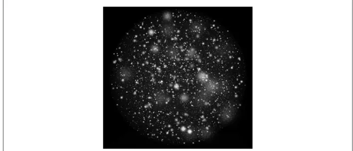
Figure 2.3: Halos data: a single time step with 1.67M particles.
large scale simulation outputs are based on advanced data reduction techniques (e.g., stratified statistical sampling [Woodring et al., 2011], compression [Rogers and Springmeyer, 2011], fea-ture extraction [Ma et al., 2007]), and re-evaluating the processes and methods that are used in visualizing such simulation outputs [Moreland, 2013].
For this thesis the target data set, consists of 250 time steps stored in individual files, is a signif-icantly smaller subset of the original simulation output. Each file includes∼16.7 million (2563) particles with 32 bytes per particle (position, velocity and mass values), and is∼537 MB in size. The particles are also tagged with unique identification numbers. Figure 2.3 shows an example of a subset of halos simulation data at a single time-step.
Chapter 3
Perceptual Consideration
In this chapter, we review factors relating to the perception of structures in three-dimensional point clouds.
Three dimensional space is interpreted by the brain based on information from the images in the two eyes. The two dimensions orthogonal to the line of sight seem relatively unproblematic since the layout of objects in the visual field corresponds to the layout of the images of those objects as projected onto the retina (albeit reversed left to right and inverted). Information about the depth dimension is more complex, being provided by a set ofdepth cueswhich are combined by the brain in various ways [Palmer, 1999]. The relative values of different depth cues depends on the nature of the data being displayed and the task [Bradshaw et al., 2000, Ware, 2012].
The so called pictorial depth cues are those that can be represented using a static perspective pic-ture. They include occlusion, linear perspective, shape from shading, and texture gradients, as well as cast shadows. None of these are likely to be very useful in the case of point clouds. For example there is little or no perspective information when the data consists of small points dis-tributed through space. Also, occlusion, a powerful depth cue, whereby objects that block the view of other objects are perceived as closer, is not effective when the objects are small points. One method for viewing point cloud data is to convert the point set to a 3D field using interpo-lation or energy functions centered on each particle [Shirley and Tuchman, 1990, Teunissen and Ebert, 2014]. This field can then be visualized using isosurface visualization or volume render-ing. In this case, the 3D shape cues of shading and ambient occlusion could be applied [Sweet
and Ware, 2004, Tarini et al., 2006]. Although turning point clouds into surfaces can sometimes be a useful technique, it suffers from the disadvantage that many structures will be hidden due to occlusion.
In the present study, we chose to study the problem of visualizing point clouds as points without the additional step of constructing a field. Another method is to replace each point with a sphere. This can provide depth cues from occlusion and shadows, but is prohibitively expensive on large scale data. In the absence of useful pictorial cues, the most powerful depth cues are structure-from-motion and stereoscopic depth. Although these have not been studied for the visualization of point cloud data, there have been a number of studies of the importance of these cues for path tracing tasks [Sollenberger and Milgram, 1993, Ware and Franck, 1996, Van Beurden et al., 2010, Naepflin and Menozzi, 2001].
3.1
Structure from Motion
Structure-from-motion is a generic term encompassing both kinetic depth and motion parallax. When a three-dimensional form (such as a bent wire) is continuously rotated around an axis and its image is projected on to a flat plane, the observer vividly perceives the 3D shape [Wallach et al., 1953] even though at any instance the only available information is two dimensional. In the computation of 3D shape from motion the brain must assume that object layout is rigid, be-cause if objects were to deform during rotating the motion due to deformation and the motion due to rotation would be impossible to separate. 3D perception from object rotation is called the ki-netic depth effect. Motion parallax is the term used to describe the shear effect that occurs when an observer moves laterally with respect to the viewpoint. For example, when an observer looks sideways out of a moving vehicle, closer objects move through the field of view faster than ob-jects at a distance. However, in some cases motion parallax and kinetic depth are essentially the same. For example, if an observer moves around an object (orbiting) while fixating that object, the resulting visual changes are the same as if the observer is fixed and the object rotates. Yet in
the former case this is called motion parallax in the latter it is called kinetic depth.
Both motion parallax and kinetic depth can be obtained through active motion of an observer. It occurs when someone moves their head laterally with respect to an object (motion parallax), or when they rotate a hand-held object (kinetic depth). It can also be obtained by means of pas-sive motion, for example when an object is set rotating in a computer graphics system. Ware and Franck [Ware and Franck, 1996] found no significance between these conditions in terms of er-rors.
But when stereo was used, the best condition overall was hand coupled object motion. Hubona et al. found no difference between active and passive conditions but for a very different task, that of 3D object matching.
3.2
Stereoscopic Viewing
The stereoscopic depth cue comes from the way the brain interprets differences (called dispar-ities) between the images in the two eyes [Howard and Rogers, 1995]. For example, in the sit-uation illustrated in Figure 3.1, where a vertical bar is fixated, an object closer to the right has less angular separation in the right eye than in the left eye. This difference is the disparity. When disparities are too large, the brain is unable to fuse the two images and observers may perceive duplicated features, or one of the features may be suppressed. The area within which fusion can occur is calledPanum’s fusional area.
Various computer graphics tools and techniques are currently available to realize stereoscopic viewing conditions. One method is the use of different polarization on different rows of pixels. If the left and right eye images are interleaved correspondingly stereoscopic depth is obtained when appropriately polarized glasses are worn [Lazzaro et al., 1998]. To generate these images, polar-izing filters that have different angles of polarization are applied to encode pairs of stereoscopic images. A polarized stereoscopic system uses special glasses to provide three-dimensional
im-Figure 3.1: Stereoscopic depth is perceived from disparities between features imaged on the retinas in the two eye. The diagram shows the situation when two vertical bars are viewed on a stereo display monitor.
ages to each eye of the users by restricting the light that reaches each eye [Wikipedia, 2016,Light, 1989, Sheiman, 1988]. If the left and right eye images are shown an alternating lines of the moni-tor, and polarized differently, stereoscopic depth is obtained when appropriately polarized glasses are worn. Another method is to use shutter glasses synchronized with the frame buffer refresh cycle which allows for different images to be shown to the left and right eyes in alternation. Fig-ure 3.1 shows the situation when two vertical bars are viewed on a stereo display monitor, and the stereoscopic depth is perceived from disparities between the features imaged on the retinas in the two eye.
3.3
Multiple Cues
A number of studies have investigated the relative benefits of motion and stereoscopic viewing. Most of these involved path tracing tasks. In some studies the stimuli consisted of wiggly lines connecting points in 3D space and the task was to find the correct terminus for a line with a high-lighted start point [Naepflin and Menozzi, 2001, Van Beurden et al., 2010]. In other studies the stimuli consisted of tree or graph structures where the task was to determine whether a short path connected a pair of highlighted nodes [Sollenberger and Milgram, 1993, Ware et al., 1993, Ware
and Franck, 1996, Ware and Mitchell, 2005, Hassaine et al., 2010].
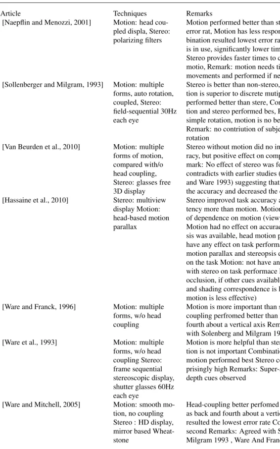
In six of these seven studies, motion was found to be a more effective cue than stereoscopic depth in terms of accuracy, when either one or the other cue was provided [Naepflin and Menozzi, 2001, Van Beurden et al., 2010, Sollenberger and Milgram, 1993, Ware et al., 1993, Ware and Franck, 1996, Ware and Mitchell, 2005]. In most of them the combination of motion and stereo depth was found to be the most effective of all. The exception is a study by Hassaine et al. that found a benefit for stereo viewing but not for motion [Hassaine et al., 2010]. They used a task identical to Ware and Frank but varied the viewpoint density [Ware and Franck, 1996]. Viewpoint density is the angular distance with which new views are provided during lateral head move-ments. However, a number of studies found that responses in stereoscopic viewing were faster than when structure from motion was the only cue (e.g. [Sollenberger and Milgram, 1993,Naepflin and Menozzi, 2001, Ware and Franck, 1996]. Table 3.1 provides a summary of studies concerning the effect of motion, stereo and their combination.
The path tracing task for 3D node-link diagrams seems similar to the problem of perception of structures in point clouds, because in both cases pictorial depth cues are unlikely to produce much benefit. For tasks other than path tracing, the relative values of different cues are likely to be different [Norman et al., 1995, Wanger et al., 1992, Hubona et al., 1997]. For example, visu-ally guided reaching for objects may be better served by stereoscopic depth than motion paral-lax [Arsenault and Ware, 2004]. Indeed, one of the main purposes of stereoscopic depth percep-tion may be to support eye hand coordinapercep-tion. There are also cases where stereo and mopercep-tion may not lead to improved task performance. For example Barfield and Hendrix [Barfield et al., 1997] found no benefit to either stereo or motion cues when the task was matching objects seen in a VR headset to objects drawn on paper. However, they did report that stereo and motion gave them an enhanced sense ofpresence. IJsselsteijn et al., found that motion contributed more than stereo viewing to a sense of presence [IJsselsteijn et al., 2001].
high performance computing (HPC) [Ahrens et al., 2014]. Briefly: because the compute power of cutting edge HPC systems is outpacing the speed at which extreme datasets can be written to permanent storage, it is becoming increasingly difficult to save sufficient data to support post-simulation analytic visualization [Ahern et al., 2011]. The solution to this problem is the com-putation of visualization products, such as images, in-situ along with the model comcom-putation. These visualizations can be much more compact than the complete checkpoint-restart frames (a complete model state dump) that have been until recently the basis for most visualization. But if images are the basis for motion parallax information, then many images will be needed. From a storage perspective, fewer images are more desirable, so it is important to know how few images can be used in order to still get a benefit from kinetic depth.
Article Techniques Remarks [Naepflin and Menozzi, 2001] Motion: head
cou-pled displa, Stereo: polarizing filters
Motion performed better than stereo in terms of error rat, Motion has less response time, Com-bination resulted lowest error rate, When stereo is in use, significantly lower time to complete, Stereo provides faster times to completion then motio, Remark: motion needs time consuming movements and performed if necessary [Sollenberger and Milgram, 1993] Motion: multiple
forms, auto rotation, coupled, Stereo: field-sequential 30Hz each eye
Stereo is better than non-stereo, Rotational mo-tion is superior to discrete mutiple angle, Momo-tion performed better than stere, Combination of mo-tion and stereo performed bes, Remark: When simple rotation, motion is no better than stere, Remark: no contriution of subject-controlled rotation
[Van Beurden et al., 2010] Motion: multiple forms of motion, compared with/o head coupling, Stereo: glasses free 3D display
Stereo without motion did no increase the accu-racy, but positive effect on completion time Re-mark: No effect of stereo was found on accuracy, contradicts with earlier studies (Solenber 1993 and Ware 1993) suggesting that stereo improved the accuracy and decreased the completion time
[Hassaine et al., 2010] Stereo: multiview
display Motion: head-based motion parallax
Stereo improved task accuracy and reduced la-tency more than motion. Motion has no evidence of dependence on motion (viewpoint density) Motion had no effect on accuracy when stereop-sis was available, head motion parallax did not have any effect on task performance. benefit of motion parallax and stereopsis depends greatly on the task Motion: not have any additive effect with stereo on task performace Explanation: less occlusion, if other cues available (e.g., perpective and shading correspondence is less difficult and motion is less effective)
[Ware and Franck, 1996] Motion: multiple
forms, w/o head coupling
Motion is more important than stereo Head-coupling perfromed better than rocking back and fourth about a vertical axis Remarks: Agreed with Solenberg and Milgram 1993
[Ware et al., 1993] Motion: multiple
forms, w/o head coupling Stereo: frame sequential stereoscopic display, shutter glasses 60Hz each eye
Motion is more helpful than stereo, type of mo-tion is not important Combinamo-tion of stereo and motion performed best Stereo contributed sur-prisingly high Remarks: Super-additivity of depth cues observed
[Ware and Mitchell, 2005] Motion: smooth
mo-tion, no coupling Stereo : HD display, mirror based Wheat-stone
Head-coupling better perfomed than others such as back and fourth about a vertical axis Motion resulted the lowest error rate Combination is the second Remarks: Agreed with Solenberg and Milgram 1993 , Ware And Franck 1996,
Table 3.1: Summary of studies concerning the effect of motion, stereo and their combination. Motion has been found to be a more effective cue than stereoscopic depth in terms of accu-racy, when either one or the other is available.
Chapter 4
Human Factors Experiments
In order to support stereoscopic viewing it is necessary to save pairs of images. But in order to support kinetic depth perception it is necessary to save entire sequences of images from a set of viewpoints orbiting a feature of interest, and for reasons of compactness. To investigate the cost benefit tradeoffs, the first experiment was designed to look at the issue of the number of unique frames needed to support kinetic depth perception and also the relative benefits of kinetic depth and stereoscopic depth. The second experiment was designed to look at the amplitude of oscilla-tion for the kinetic depth effect.
Using structure-from-motion cues in scientific visualization applications can lead to a problem of viewpoint preservation. People often wish to contemplate a structure from a particular viewpoint, but rotation causes a continuously change in the viewpoint. A partial solution is to generate ki-netic depth by oscillatory rotation about a fixed axis. If the amplitude of oscillation is relatively small then the viewpoint can be approximately preserved. We generate oscillation using the func-tion shown in Figure 4.1.
Angleof Rotation=α∗sin(t∗2π/λ)
whereαis the amplitude of oscillation andλis the period of oscillation. Figure 4.1: The function used for generating oscillatory rotation
Our hypotheses are shown in Table 4.1. We also measured response times, but did not generate formal hypotheses for this variable.
H1: Kinetic depth will improve target detection in point cloud data. H2: Stereo viewing will improve target detection in point cloud data.
H3: Kinetic depth will be more effective than stereo viewing in improving target detection in point cloud data when motion is smooth.
H4: The value of kinetic depth will be reduced for lower update rates.
H5: The value of kinetic depth will be reduced for smaller amplitudes of motion. Table 4.1: Hypotheses
4.1
Experiment 1
The objective of the first experiment was to discover the relative benefits of stereo and motion viewing conditions in the detection of three-dimensional patterns in point clouds. The approach taken was to use artificial point clouds resembling the halos computed by domain scientists. Us-ing artificial rather than real data makes it possible to generate large number of trials contain-ing unique patterns. Artificial targets were placed within the point clouds, and study participants were trained to detect them.
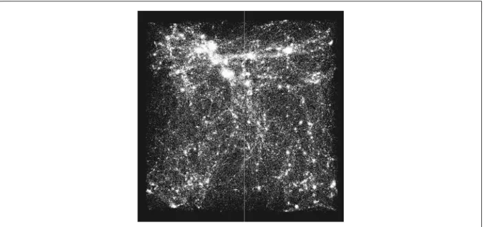
Figure 4.2 shows a sample view of the artificialuniverseconsisting of 1.63M particles. The whole scene was either stationary or in oscillatory motion. The motion was generated by rotating around a central vertical axis at the center of the point cloud using the equation in Fig-ure 4.1. The period of oscillation was 2 seconds. and the amplitude of oscillation was 15.0 de-grees.
4.1.1
Conditions
Six distinct redraw rates were compared (0, 3, 6, 15, 30, and 60 updates per second). There were also two viewing conditions: stereo display and no-stereo display. A redraw rate of zero results in no motion so this is provides a condition with no kinetic depth.
Figure 4.2: Artificially generated background consist of 1.63M particles in 3D space
4.1.2
Test Patterns
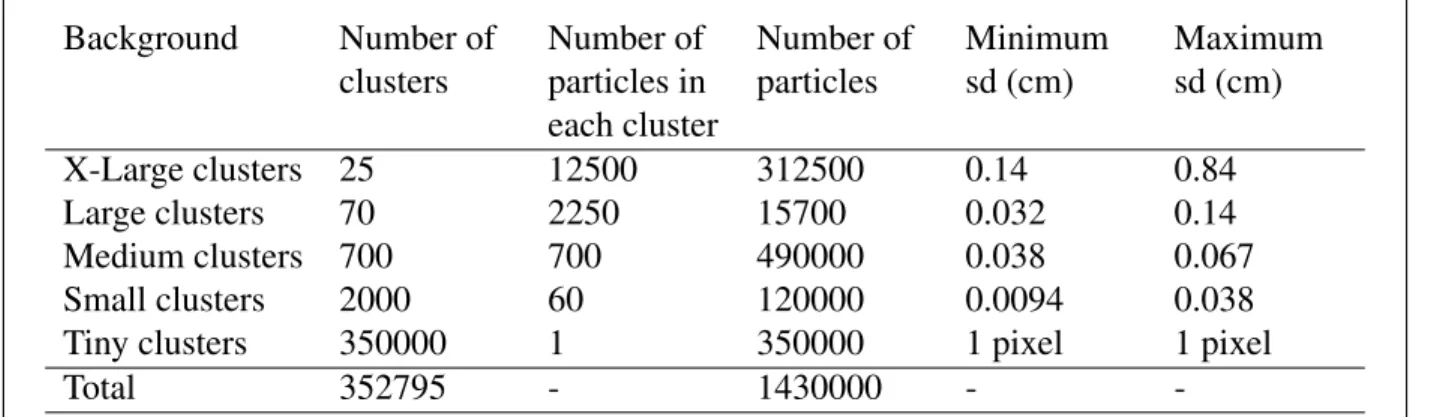
Our test data was artificially generated to have some of the qualities of dark matter simulations. To provide a backgrounduniversefor the target features five distinct sizes of point clusters were generated and randomly positioned in the sphere as described in Table 4.2.
Each cluster contained the number of points specified normally distributed with the specified standard deviation. The background had radius of 16.0 cm. All points were rendered as pixels with a transparency of 0.2.
On a given trial there was either no target, or one of three types of target pattern was generated and randomly placed within the background field within a radius of 0.75 of the overall radius. The three target patterns were as follows:
1. Filament:A set of clusters on a natural cubic spline. The spline path was drawn through five control points which were randomly chosen from a spherical space having a radius 3.8 cm. Seven clusters (2 large, 2 medium and 3 small) were uniformly distributed along the spline path.
2. Satellite:Cluster with multiple satellite of clusters. A cluster of points was generated using 7500 points normally distributed with a standard deviation of 0.28 cm. Ten satellite clusters (4 large, 3 medium and 3 small) were randomly positioned around the center cluster at a distance of 1.2 cm
3. Enhanced filament:Enhanced pattern based on double filaments. Two filaments were constructed. A cluster of 4500 particles (sd=0.32 cm) was positioned at their point of in-tersection.
Examples of the three target pattern types are given in Figure 4.3.
Background Number of clusters Number of particles in each cluster Number of particles Minimum sd (cm) Maximum sd (cm) X-Large clusters 25 12500 312500 0.14 0.84 Large clusters 70 2250 15700 0.032 0.14 Medium clusters 700 700 490000 0.038 0.067 Small clusters 2000 60 120000 0.0094 0.038
Tiny clusters 350000 1 350000 1 pixel 1 pixel
Total 352795 - 1430000 -
-Table 4.2: Parameters used to generate background data
The code that we used to generate the dataset can be reached through the code repository link provided on Appendix C.
4.1.3
Task
The participants’ task was to respondYESorNOdepending on whether they detected a target in the background pattern. The display was presented for two seconds, and then the screen was cleared. They responded using one of two specially marked keys on the keyboard. [Yes] (Over-laid on the V-key) if the pattern was present and [No] (over(Over-laid on the N-Key) if it was not. Par-ticipants were instructed to leave their left index finger on the [No] key and the right index finger on the [Yes] key.
(a) Filament (b) Satellite (c) Enhanced Filament Figure 4.3: Sample structures randomly created on three-dimensional space.
4.1.4
Participants
There were 14 participants (12 females and 2 males) on the first experiment. They were paid for participating.
4.1.5
Procedure
There were 36 main conditions (6 redraw rates x 3 test patterns x stereo vs no stereo). Trials were given in blocks of 60 for each test pattern. Each block was constructed of 5 trials at each redraw rate with the target present and 5 at each redraw rate with the target absent. All the trials in a block of 10 had the same type of target patterns, although the actual target pattern was gener-ated for each trial based on random parameters. The first three blocks used the three different test patterns given in a random order, and this was repeated with a new random order. There were six trial blocks for the stereo condition and six for the no-stereo condition with stereo and no-stereo conditions being given on different days, randomly assigned as stereo first and no-stereo first. Overall there were 720 trials (10 target-present trials and 10 target-absent trials in each of the 36 main conditions).
re-duced set of conditions. Only three of the redraw rates were used (60, 15, 0) and there were 6 trials per condition. In this phase participants were given directions on what to look for and cor-rected when they made an error. Prior to each trial block, participants were shown two examples of the target pattern with no simulated halos background.
4.1.6
Display/Hardware
Stereoscopic imagery was presented using a frame sequential display with alternating left and right eye images and synchronized shutter glasses, each eye receiving a 60 Hz refresh rate. The perspective was based on a viewing distance of 75 cm from the screen and the experimenter was instructed to seat participants at this distance. The center of the simulated universe was place a further 20 cm behind the screen.
The hardware consisted of a NVIDIA Quadro 4000 graphics card, NVIDIA 3D Vision P854 Wireless Active 3D Glasses and Acer HN274H 1920x1080@120 Hz monitor with a screen 59.3 cm x 33.6 cm.
4.1.7
Results
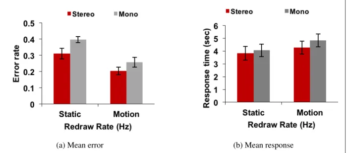
One of the 14 participants had an exceptionally high error rate, performing at chance on some conditions. That data was removed and the analysis was done based on data from the remaining 13 participants. Figure 4.4 summarize the results from the first experiment.
As Figure 4.4a illustrates, error rate performance for stereo was always better than performance with no-stereo for a given update rate. The error data were subjected to a 2-way repeated mea-sures ANOVA (redraw rate x stereo/no-stereo). Hypotheses H1,H2 and H4 were supported. There were highly significant main effects for both redraw rate [(F[5,60]=26.9, p<0.001) and stereo/no-stereo (F[1,12]=27.9, p<0.001). There was also a significant interaction (F[5,10]=3.2, p<0.05 with a Greenhous-Geisser sphericity correction). The interaction suggests that the benefit of
(a) Mean error (b) Mean response
Figure 4.4: Experiment 1 results. Vertical bars represent 95% confidence intervals.
stereoscopic display decreases as the motion becomes smoother.
The response time data were subjected to a 2-way repeated measures ANOVA (redraw rate x stereo/no-stereo). There were significant main effects for both redraw rate (F[5,60]=5.93, p<0.01) and stereo/no-stereo (F[1,12]=5.77, p<0.05) (both with Greenhouse-Geisser sphericity correc-tion). There was no significant interaction. The time to respond was shorter (on average by ap-proximately 630 ms) for stereo viewing. Response times increased with the redraw rate.
4.2
Experiment 2
The goal of the second experiment was to determine how target detection varied with the ampli-tude of the motion. Because small ampliampli-tude motion is desirable, we were interested in finding out how much amplitude could be reduced before performance declined significantly. In most respects the procedure was the same as for the first experiment. The same method was used to generate both the background point field and the target patterns. In all conditions the redraw rate was 30 Hz.
4.2.1
Conditions
Six amplitude (angle of rotation) values were compared (0, 1, 2, 3, 8, and 16 degrees) both with and without stereo viewing. Error rate and time to respond were dependent measures.
Trial blocking was the same as for the first experiment, with the different amplitudes of motion substituted for the different redraw rates. As with the first experiment the experiment was run over two different sessions with stereo for one session and no stereo for the other (order ran-domly selected).
4.2.2
Participants
There were 14 participants (5 females and 9 males) on the second experiment. They were all paid for participating.
4.2.3
Results from Experiment 2
Figure 4.5 summarize the results from the second experiment. As Figure 4.5a illustrates, er-ror rate performance for stereo is always better than performance with no stereo for a given up-date rate. The error data were subjected to a 2-way repeated measures ANOVA (amplitude x stereo/mono). There were highly significant main effects for both amplitude (F[5,65]=22.7, p <0.001) and stereo/mono (F[1,13]=39.3; p<0.001). There was no significant interaction. The response time data were subjected to a 2-way repeated measures ANOVA (redraw rate x stereo/mono). There was significant main effects for amplitude (F[5,60]=14.6, but no significant effect for stereo/mono. There was a significant interaction effect (F[5,65] = 2.19; p<0.05 with Greenhouse-Geisser correction). Greater amplitudes resulted in slower responses.
(a) Mean error (b) Mean response
Figure 4.5: Experiment 2 results. Vertical bars represent 95% confidence intervals.
4.3
Meta-Analysis
Four of the conditions from the two experiments were close to identical. Both experiments had identical stereo and no-stereo conditions with no motion. Experiment 1 had conditions with an amplitude of 15 degrees and 30 Hz update rate (stereo and no-stereo). Whereas Experiment 2 had the same conditions with an amplitude of 16 degree. Accordingly we combined the data for these conditions yielding 27 participants. The results are summarized in Figure 4.6a and Figure 4.6b. We subjected this to a 2-way repeated measure ANOVA for errors. There was a main effect for stereo/mono (F[1,26] = 142.9; p<0.001) and a significant main effect for motion (F1,26] = 37.0; p<0.001), with no interaction. The overall effect of stereo was a 21% reduction in errors. The overall effect of motion was a 35% reduction in errors. Combining motion and stereo viewing reduced errors by 49%.
Figure 4.6b shows time to respond results. A two-way repeated measures ANOVA revealed main effects for both stereo/mono (F[1,26]=142; p<0.001) and for motion (F(1,26)=36.9; p<0.001) with no interaction. Having stereo resulted in faster responses, but having motion resulted in slower responses.
(a) Mean error (b) Mean response
Figure 4.6: Experiment 1 and 2 results combined. Vertical bars represent 95% confidence intervals.
4.4
Discussion
This study has been the first to look at the relative values of stereo and motion cues for the task of finding features in point cloud data. It suggests that both kinetic depth and motion are useful cues for helping people find features in point clouds, and they should be applied wherever possi-ble. The utility of motion was found to increase with amplitude, but good results were found for amplitudes of 4 degrees and greater.
The results are broadly in agreement with previous studies using path tracing tasks. As discussed in our introduction six of seven prior studies found structure-from-motion to be a more powerful cue than stereoscopic viewing in terms of error rates for the task of tracing 3D paths. Also like some of these prior studies we found that structure-from-motion increased response times. Motion was not a stronger cue for all conditions, its value was found to vary strongly with both the number of distinct frames per second and the amplitude. Motion was only a more effective cue for amplitudes greater than 4 deg and with update rates of at least 15 Hz. The majority of
prior experiments have only used a single motion condition and a single stereo condition (an ex-ception is [Hassaine et al., 2010]). As a broad comment on these kinds of experiments, general statements, such as motion was a more powerful cue than stereo, must always have the caveat for the particular viewing conditions used. Obviously if motion is very slow, or much too fast its value will be minimal.
There are also different stereo viewing parameters that can be adjusted. For example, virtual eye separation can be adjusted to increase or decrease disparities [Ware et al., 1998]. It might be thought that enhancing disparities is the best approach, but because Panums’ fusional area can be small, reducing virtual eye separation may be better if the features of interest have a substantial depth extent.
These kinds of consideration all suggest that for any given visualization design, many factors must be considered. Are the users likely to be willing to invest in stereo viewing hardware? If not, motion is really the only option for enhancing raw point cloud data. Is target detection the paramount consideration? If it is, motion and stereo viewing will be the best choice (assuming stereo is available). Is interaction necessary? If so, it may be necessary to halt motion to facil-itate selection, and in this case stereo viewing will facilfacil-itate eye hand coordination. Is the goal the presentation of results to a larger audience? In this case, we must consider the fact that stereo viewing is not yet widely available whereas the ability to show short animated movies is becom-ing ubiquitous so structure from motion is a more useful cue. On the other hand, if virtual reality headsets become widely available, then providing both cues may become commonplace.
There are many aspects of this problem still to be explored. Although we varied amplitude of oscillation and update rate, we always had the same frequency of oscillation. Also there is the issue of active and passive motion for point cloud data. There have only been a few studies of this issue with path tracing tasks and in any case, we cannot assume that the same results would be found for point cloud data with different kinds of tasks.
laser mapping technologies. In some cases there is a need to view and edit the raw data [Wand et al., 2007]. It is likely that the results we obtained for the simulated halos model data would also apply to laser scans, but this is not certain. In the case of laser mapping, the data tend to lie on distinct surfaces unlike the data we simulated and this could lead to different outcomes. In conclusion, the results from this study suggest that for the task of perceiving features in point clouds structure from motion is a more valuable depth than stereoscopic viewing, although ide-ally both could be used since the effects were found to be additive. But motion should be reason-ably smooth and if motion is oscillatory an amplitude of at least four degrees should be used.
Chapter 5
The Interactive Interface
In this chapter, a tool designed to let users interactively navigate within a point cloud dataset is proposed. The optimum viewing conditions (such as redraw rate, the form of the motion to gener-ate motion parallax, frustum dimensions, and so on) that were studied on the formal experiments discussed in Chapter 4 are taken into account. A commonly used flow visualization technique (streamlets) is implemented as a visualization method in order to represent particle and clus-ter orientations based on their position and velocities. User requirements elicited from domain experts based on a literature survey are also taken into account in the application design. In the following sections, first, the rationale for developing the interactive application is laid, and a liter-ature review concerning methods for interacting with virtual environments, specifically with point clouds, is presented. Finally, the software application developed for this thesis is described.
5.1
Rationale
One of the major goals of this thesis is to develop methods for rapidly exploring and visualizing a point cloud data set. This section outlines functional requirements derived from user expectations on performing the visual analysis task on a large point cloud dataset. The target audience is the scientists working in the field of computational cosmology.
5.1.1
Functional Requirements
The following list outlines the functional requirements in designing the interactive exploration application:
FR1: Interaction
(a) Ability to navigate the viewpoint easily and intuitively through the point cloud. (b) Ability to scale the scene up and down about a point of interest.
(c) Ability to select a subset of particles and animate their trajectories through space and time from the beginning of the modeled universe to the present.
FR2: Data management.
In order to provide visualization and interactive exploration of such a large scale dataset, which consists of particle samples distributed into separate time step files, a data manage-ment method for efficiently dealing with the dataset is needed. A solution likely to be in a form of indexing and spatial partitioning. The system should support a structure such that, as the system user navigates within the data set, the desired set of particle values should efficiently be pulled from the corresponding data file.
FR3: Visualization parameters
(a) Representing particle velocities
A method is needed to represent both the speed and 3D direction of particles in the point cloud.
(b) Tracing particles over time
Visualizing traces of particles or clusters within a spherical point of interest (rep-resents a focal area of interest as if the user is holding a 3D scope inside the virtual world) is desired. Observations of clustering events of halos, such as their birth, death,
merge, split and continuation, should be observed. To do this, retrieving the traces of particle clusters from the multiple time-steps is also required, as the data is stored in separate files for each time step.
(c) Support for optimum viewing parameters
In Chapter 4, two formal experiments evaluated perceptual requirements for perceiv-ing 3D structures in point clouds. The system should consider the parameters tested in these studies. First, an auto-rotation of the whole scene with a type of oscillatory (or rocking) fashion to enable the contribution of depth cues (kinetic depth, motion paral-lax) should be available. Second, the system user may choose to utilize stereoscopic viewing features, and the system should support appropriate stereoscopic viewing pe-ripherals, such as shutter glasses, high resolution computer monitors and projectors that support over 120Hz refresh rates.
FR4: Software Considerations
There are a number of open source efforts that aim to provide visual analysis solutions for data intensive analytics needs. O The system architecture designed as part of this thesis should be compliant with the pipeline structure, so that the artifacts of this thesis, the inter-active application, could be turned into modules (data reader, renderer), which can be then integrated into one of these libraries as a plug-in. Secondly, the system should utilize GPU programming to parallelize calculations (such as velocity representation calculations) when possible for optimization and improved performance.
5.2
Literature Review
The fundamental forms of interaction in a computer-generated world can be categorized into four basic actions: navigation, selection, manipulation and data input by a system user [Mine, 1995]. These actions can be performed in a variety of modes, such as direct user interactions
(e.g., hand tracking, gesture recognition, pointing, gaze direction) or through using controllers which can be virtual or physical (e.g., buttons, touchpads, pens, sliders, dials, joysticks, wheels). Figure 5.1 presents different methods and devices that are developed to interact with scientific datasets. However, the methods to interact with a virtual environment depend on not only the task at hand but also the structure of the dataset. Therefore, the interaction method should ideally be designed for the specific nature of the dataset and the features of interest within it. The follow-ing section presents a literature survey of interaction methods that are related to the problems of viewing point cloud datasets. Also considered are open source software libraries and toolkits that are commonly used in handling large scale point cloud datasets to develop visual analysis appli-cations.
5.2.1
Interacting with Point Clouds
A number of techniques have been developed to interact with 3D objects in virtual worlds. Most of the studies are based on spatial selection and involves driving a ray into the scene towards the object of interest from the user’s cursor until it intersects with the surface of the object [Pierce et al., 1997, Hand, 1997, Zeleznik et al., 1997]. In computational geometry, this method is recog-nized as ray-surface intersection or ray-casting. Grossman et al. provide an extensive survey of 3D selection techniques based on ray casting for volumetric displays [Grossman and Balakrish-nan, 2004].
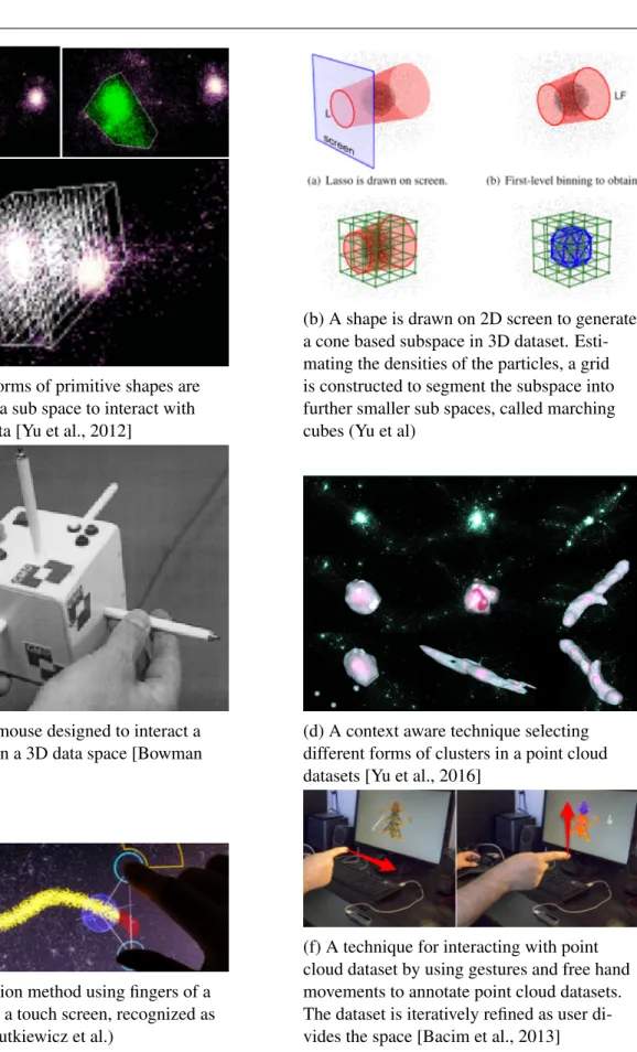
There are also methods developed to interact specifically with point cloud [Wiebel et al., 2012, Remondino, 2003, Scheiblauer, 2014, Bacim et al., 2014] The common idea of these techniques is based on a spatial specification of a sub-space that contains the elements to be further explored. In order to make interaction simpler, these subspaces are defined using primitive geometric forms, such as cones, cubes, circles, lasso, polygons, which usually do not exist within the original data [Liang and Green, 1994,Pfister et al., 2000,Bowman et al., 2001,Steed and Parker, 2004,Yu et al., 2016, Valkov et al., 2011, Shan et al., 2012]. Figure 5.1a shows examples of simple geometric
shapes that are commonly used to define a sub space to interact with point cloud data.
A group of methods involve free-hand gestures; however, these techniques require dedicated 3D input devices. For example, Bacim et al. used sub spaces controlled through 3D gestures Fig-ure 5.1f. Butkiewicz et al. use a multi-touch based 3D positioning in a form of coupling fingers and the cursor to manipulate the 3D subspace for this purpose [Butkiewicz and Ware, 2011]. Fig-ure 5.1e shows this technique (pantograph) in use. Others used 3D mice, optical tracking devices and so on. For example, Figure 5.1c shows a cubic mouse designed to manipulate a virtual object in 3D space by using a cube-shaped device with three rods coupled with primary axes [Frohlich and Plate, 2000, Bowman et al., 2001]. Another example, Cabral et al positioned a cube with two handed sphere [Cabral et al., 2014].
Another group of techniques use conventional user pointing devices, such as mouse and key-board, to manipulate subspaces in the virtual environment by using geometric shapes calculated as a function of user inputs and predefined geometric forms. For example, Wiebel’s method al-lows users to select spatial position in volumetric renderings by simply enclosing an area of in-terest by drawing a free form shape on the 2D projection of the 3D dataset, which is then used to derive a sub-space within the volume [Wiebel et al., 2012]. Another example is Yu et al.’s method presented in Figure 5.1b [Yu et al., 2012]. This method is based on a shape drawn on the 2D screen to define a cone based subspace in a 3D dataset. Then a grid is constructed by estimat-ing densities of the particles inside it, in order to segment the sub-space into further smaller sub spaces. A grid constructed in the box of selected area, and a smaller cubes are used to enclose sub areas to further investigate (Figure 5.1a). An enhanced version of this approach is also avail-able that a solution utilizes scoring functions to interactively constraint the area of interest (or the sub-space) as the user navigates within the dataset [Haan et al., 2005].
One form of ray-casting technique is based on progressively reducing the set of selectable objects to refine the area of interest to make the selection task with lower precision [Kopper et al., 2011]. However, for point cloud datasets, object selection methods do not apply because groups or