UC Davis
IDAV Publications
Title
Visualization Techniques for Time-Varying Volume Data
Permalink
https://escholarship.org/uc/item/50h5580f
Authors
Ma, Kwan-Liu
Lum, Eric
Publication Date
2001
Peer reviewed
eScholarship.org
Powered by the California Digital Library
University of California
CAD/Graphics’2001 August 22-24, Kunming
International Academic Publishers
STRATEGIES FOR VISUALIZING TIME-VARYING VOLUME DATA
Kwan-Liu Ma
and
Eric Lum
Department of Computer Science, University of California
Davis, CA 95616-8562, U.S.A.
E-Mail: {ma,lume}@cs.ucdavis.edu
ABSTRACT
Our ability to study and understand complex, transient phenomena is critical to solving many scientific and engi-neering problems. This paper addresses the issues in stor-age space, I/O, and rendering for visualizing time-varying volume data. A suite of effective techniques, including en-coding, parallel rendering, and runtime visualization tech-niques are discussed. In particular, we introduce a new hardware-assisted technique coupled with a compression scheme based on Discrete Cosine Transform which allows interactive exploration in both spatial and temporal do-mains of the data using a PC with a commodity graphics card.
KEYWORDS: high performance computing, compression, parallel rendering, PC, pipelining, remote visualization, scien-tific visualization, spatial data structures, texture hardware, time-varying data, volume rendering
INTRODUCTION
Time-varying volume data sets, which may be obtained from numerical simulations or remote sensing instru-ments, provide scientists insights into the detailed dynam-ics of the phenomenon under study. Examples include data from the study of neuron excitements, crack propagation in a material, evolution of a thunderstorm, unsteady flow surrounding an aircraft, seismic reflections from geologi-cal strata, and merging of galaxies. A typigeologi-cal time-varying data set from a computational fluid dynamics simulation can contain hundreds of time steps and each time step can have more than millions of data points. Generally, mul-tiple values are stored at each data point. As a result, a single data set can easily require hundreds of gigabytes storage space, which creates challenges to the subsequent data analysis tasks.
The ability of scientists to visualize time-varying phe-nomena is absolutely essential to ensure correct interpre-tation and analysis, to provoke insights and to communi-cate those insights with others. For instance, by directly and appropriately rendering a time-varying data set, we can produce an animation sequence that illustrates how the underlying structures evolve over time. In particular, interactive visualization is the key which allows scientists to freely explore in both spatial and temporal domains, as well as in the visualization parameter space by changing view, classification, colors, etc.
In this paper, we discuss how time-varying volume data sets can be efficiently rendered to achieve interactive visu-alization. First, careful encoding of the data can not only reduce storage requirements but also facilitate subsequent rendering calculations. Second, coupling visualization ca-pabilities into a time-dependent simulation makes possible more intuitive tracking and tuning of simulation parame-ters while simulation is running. Next, rendering calcula-tions can be parallelized to increase rendering rate while maintaining high image quality, but the I/O issue must be addressed so the display rate can keep up with the ren-dering rate. Both a pipelined approach and a compression strategy are suggested for reaching the highest possible ef-ficiency. Finally, we describe how to use a low-cost PC graphics card to render time-varying volume data for in-teractive data exploration.
TIME-VARYING VOLUME DATA
Besides being large, certain aspects of time-varying vol-ume data require special attention for visualization. First, data quantization is often done for visualization to cope with limited color precision or storage space. Further-more, non-uniform quantization helps enhance particular features in the data. Since the dynamic range of data val-ues in a time-varying data set may vary over time stepsTable 1: Four Test Data sets.
data set time steps spatial resolution Turbulent vortex flow 100 1283
Turbulent jet flow 150 1283 Quasigeostrophic 1400 2563 turbulent flow
Shock-bubble flow 265 640256256
by as much as several orders of magnitude, quantization becomes a less trivial job.
Second, features of interest in a time series may exhibit a regular, periodic, or random pattern. A regular pattern is characterized by a feature that moves steadily through the volume. The structure of the feature neither varies dra-matically nor follows a periodic path. Features exhibiting a periodic pattern appear and disappear over time. Tran-sient features of interest or features that fluctuate randomly are very common, such as those found in turbulent flows. Generally, regular and periodic patterns can be more easily detected and more efficiently rendered.
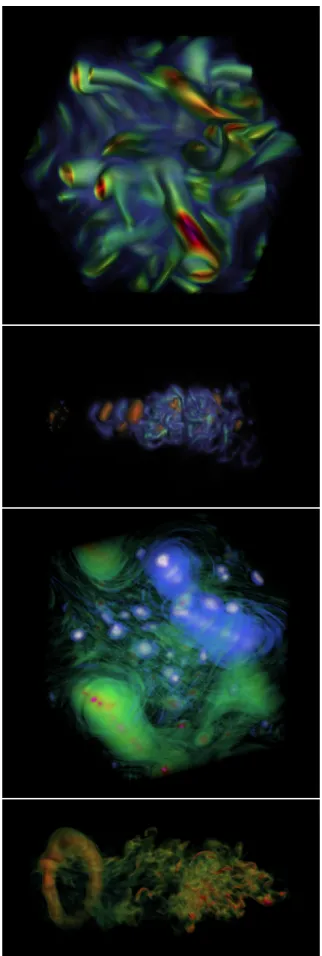
Table 1 lists the four data sets that have been used for our study. Figure 1 shows one frame from each data set. An animation of the turbulent vortex flow data displays a fairly random pattern over time as the vortices spread the whole domain. In the turbulent jet data, we see more pe-riodical behaviors isolated in a relatively small space. We also see a more periodic pattern in the quasigeostrophic turbulence data. The shock-bubble flow data exhibits a slowly developing structure starting from one end of the domain and eventually reaching the other end of the do-main.
ENCODING
Based on the characteristic of each time-varying volume data set, the storage requirements and rendering cost of the data may be significantly reduced with proper encod-ing. Shen and Johnson [17] develop a ray-cast rendering strategy which they call differential volume rendering. By exploiting the data coherency between consecutive time steps, they are able to reduce not only the rendering time but also the storage space by 90% or more for their two test data sets which are highly temporally correlated and contain spatially coherent byte data. Differential volume rendering is potentially parallelizable.
Based on similar concepts, Westermann [18] performs wavelet encoding of each time step separately to gener-ate a compressed multiscale tree structure. Feature extrac-tion and tracking as well as further compression can be obtained by examining the resulting multiscale tree struc-tures and wavelet coefficients. Using wavelet transform
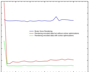
0 5 10 15 20 25 30 Time Step 0.0 1.0 2.0 3.0 4.0 5.0 6.0 Time in Seconds
Total Rendering Cost
Brute−force Rendering
Rendering encoded data but without octree optimizations Rendering encoded data with octree optimizations
Fig. 2: Rendering cost for each of the first 30 time steps of the turbulent jet data set. The time is the total time to process, including reading encoded data from disk, un-encoding when necessary, calculating gradient, rendering and compositing. Octree optimization allows skipping of transparent regions as well as accelerated rendering of non-transparent uniform space.
offers an underlying analysis model to characterize time-varying data.
Quantization is probably the simplest encoding we can do. Ma and Shen [10] discuss how non-uniform quantiza-tion along with octree and difference encoding can be done to speed up rendering of time-varying volume data. The octrees for consecutive time steps can be merged to share subtrees. Consequently, during rendering, partial images built from subtrees that have not changed over time may be reused in the following time steps. Figure 2 shows the cost of rendering the turbulent jet data set with encoding using a SUN Ultra Sparc workstation.
Wilhelms and Van Gelder [20] design hierarchical data structures for controlled compression and volume render-ing. They extend octrees and a branch-on-need (BON) subdivision strategy [19] to handle multi-dimensional data. The basis of their work is a hierarchical data model, and the resulting multi-dimensional tree stores a model of the data and evaluation information about the error of the model as well as importance of the data to control com-pression rate and image quality. Nevertheless, 4-d octrees are not ideal for organizing time-varying data. The spatial and temporal resolutions could be very different, and this discrepancy makes it difficult to locate the temporal co-herence in certain regions. Another problem of using 4-d trees is that coupling spatial and temporal domains makes it difficult to locate regions with only temporal coherence
but not spatial coherence.
Shen, Chiang, and Ma [16] introduce a hierarchical data structure, called Time-Space Partitioning (TSP) tree, for a better utilization of both spatial and temporal coherence. In essence, the skeleton of a TSP tree is a standard com-plete octree, which recursively subdivides the volume spa-tially until all subvolumes reach a predefined minimum size. To store the temporal information, each TSP tree node itself is a binary tree. Every node in the binary time tree represents a different time span for the same subvol-ume in the spatial domain. The focus of the algorithm is to reduce the amount of data required to complete the render-ing task and to reduce the volume renderrender-ing time. In par-ticular, TSP trees allow the renderer to use data from sub-volumes of different spatial and temporal resolutions. The TSP tree data structure has been also used by Ellsworth, Chiang, and Shen [3] to facilitate large scale volume ren-dering using 3-d texture hardware.
RUNTIME VISUALIZATION
Scientists typically run large-scale time-dependent simula-tions on parallel supercomputers operated at a remote site, like a national supercomputer center. Moving a complete time-varying data set from the supercomputer center to the scientist’s own computing laboratory for data analysis and visualization, if not possible, can be very troublesome.
A good approach to this problem is based on a runtime visualization scenario. That is, visualizing time-varying data probably can be done most efficiently while the data are being generated, so that users receive immediate feed-back on the subject under study, and so the visualization results can be stored rather than the much larger raw data. Runtime visualization of time-dependent simulations has been demonstrated by several researchers. Rowlan [14] and Ma [8] independently demonstrated runtime tracking of three-dimensional numerical simulations using direct volume rendering on a massively parallel computer. VI-SUAL3 [5] and SCIRun [13] are among a few software systems that can support runtime tracking. These systems can be operated in a distributed computing environment.
However, runtime tracking is not always possible and desirable for certain applications. For example, one may want to explore the data set from different perspectives; or, the amount of computation power required for real-time rendering or a special visualization technique may not be readily available. In addition, competing with the numer-ical simulation to perform visualization calculations for computing time and memory space on the same parallel supercomputer is sometimes not acceptable by scientists.
PARALLEL
POST-PROCESSING
VISUALIZATION
To achieve interactive visualization that is key to effec-tive data exploration, further speedup of rendering may be made by utilizing parallel computers or graphics hardware. However, even though a parallel computer can render at multiple frames per second, without high-speed network and parallel I/O support, two bottlenecks can still make it impossible to achieve interactive viewing. One bottleneck is the need to read large files continuously or periodically throughout the course of the visualization process. The other is the delay due to transferring the resulting images over a non-dedicated network.
Ma and Camp [9] develop a post-processing parallel vi-sualization strategy based on pipelined rendering. They demonstrate remote visualization of time-varying volume data on a PC cluster over a wide-area network. Pipelin-ing and careful groupPipelin-ing of processors are used to hide I/O time and to maximize processor utilization. Visually lossless compression is used to significantly cut down the cost of transferring output images from the PC cluster to a display device through a wide-area network. Both tests between NASA Ames Research Center and UC Davis, and tests between a research laboratory in Japan and UC Davis show the display rates can mostly keep up with the render-ing rates.
This post-processing of pcalculated data actually re-mains a common practice, and the scenario is that the scientist leaves the data on the supercomputer center’s mass storage device, retrieves them to perform visualiza-tion calculavisualiza-tions on a parallel computer at the supercom-puter center, and displays the resulting images/animations on his/her desktop computer.
HARDWARE-ASSISTED
RENDER-ING
Commodity PC graphics cards are capable of performing rendering that required a high-end graphics workstation a few years ago. In particular the 2-d texture hardware which helps generate impressive graphics for video games can also applied to make effective visualizations.
Commodity PC graphics cards have been used for vol-ume rendering of static volvol-umetric data [1] [16]. Volvol-ume rendering requires the loading of the volumetric data into the texture memory of the video card prior to rendering. The size of the volume that can be rendered is often limited by the amount of video memory the card contains since the access and transfer of data from main memory across the graphics bus is relatively slow compared to the direct ac-cess of graphics memory.
(1) Compression
The real time rendering of volumetric datasets offers a number of challenges because of the sheer size of the data being visualized. The size of this data can be reduced and therefore made more manageable through the use of compression. The advantages of compressing volumetric data are two fold. First, it reduces the storage require-ments needed for the data. This could allow a dataset to fit in texture memory that might otherwise not fit, elim-inating the need for transferring data across the graphics bus from main memory to texture memory. The reduc-tion in storage can also be used to fit relatively large com-pressed datasets entirely in main memory thus eliminat-ing the need for swappeliminat-ing from disk. The other benefit of compression is the reduction in I/O. Even if a dataset does not fit into texture memory, the transferring of com-pressed data across the graphics bus can be substantially faster than with uncompressed data, allowing for interac-tive visualization. In addition, for out-of-core rendering of very large datasets, the reading of compressed data from disk requires less time than reading uncompressed data.
Video and main memory can be thought of as a two-level cache for volume rendering. The compression of vol-umetric data not only increases the amount of data that can fit in each level, but also decreases the I/O costs of trans-fers between these levels. We believe that through the use of compression, and careful management with respect to the time costs associated with the transfers between levels, the interactive volume rendering of very large datasets is possible using commodity PC hardware.
If a compressed volume is to be used directly from video memory, it must also be uncompressed using the graphics hardware. This is a significant constraint since the opera-tions supported in video hardware are are extremely lim-ited. Another constraint is imposed by the fact it is very desirable to encode the scalar voxel values in terms of their scalar value rather than as a red, green, blue, alpha (opac-ity) set. Using scalar values and color indexed textures allows a scientist to manipulate the color palette to inter-actively change the opacity and color maps. This provides more intuitive visualization of the data. Storing voxels in terms of RGBA would require recompressing the dataset as parameters are changed which can be impractical for very large datasets. In addition, storing a single scalar value, rather than four color scalars reduces the amount of data by a factor of four.
Using indexed values puts a number of limitations on how graphics hardware can be used to decode data since most screen and texture combining operations supported in hardware work in terms of the manipulation of RGBA values and not the manipulation of scalar index values prior to being looked up in a color table. In particular, one could conceive of compression methods that would would
deal with difference images or volumes. These difference, however, would need to be combined in terms of RGBA and not indexed scalars. This would make the difference images color and opacity map depended, since the differ-ence between two volumes in terms of RGBA depends ex-tensively on the mapping being used. For example, a dif-ference in scalar value might correspond to a change in red, a change in green and blue, or perhaps no change at all, depending on the color map, and the value of the scalar the difference is being applied to.
(2) Palette Based Decoding
With these limitations in mind, we present a method for the temporal encoding of indexed volumetric data that can quickly be decoded in hardware. The method makes ex-tensive use of OpenGL’s support for the changing of color palettes without the reloading of textures. The cycling of color palettes can be used to create simple animations from static images. In our work we use color palette manipula-tion to allow a single scalar value to represent several times steps. For each frame the palette is varied to properly de-code the approximate scalar value of that voxel for that frame, which is then mapped to the desired opacity and color value for that scalar index.
With paletted textures, a single scalar value is used to represent an RGB or RGBA color. The palette consists of a limited set of colors that sample the RGBA color space. Each of these colors is encoded in a single value, often an unsigned byte. In our approach we encode a sequence of temporally changing scalar values into a single index. In this way, the index stored in a texel represents an ap-proximation for a sequence of scalar values. Each possible index value therefore represents a sample in the space of possible time varying scalar values. The scalar value that an indexed texel encodes can be decoded to its temporally changing value through the frame to frame manipulation of the palette. For each frame, the color for each index is set to the color represented by the scalar value represents during that frame.
(3) Temporal Encoding
The encoding process consists of mapping sequences of scalars into single scalar index. We perform this process using transform encoding, specifically using the Discrete Cosine Transform (DCT) [6, 4, 15]. Transform encoding is a compression method that transforms data into a set of coefficients that are then quantized to create a more com-pact representation. The transform by itself is reversible, and does not compress the data. Rather, a transform is se-lected that puts more energy into fewer coefficients, thus allowing the less important, lower energy, coefficients to be quantized more coarsely, thus using less data.
We use the DCT since it is known to have good infor-mation packing qualities and tends to have less error at the boundaries of a sequence [4]. Boundary performance is important in order to avoid discontinuities during the tran-sition between blocks. Since our application compresses temporally, discontinuities would appear in the form of flashes between compressed sequences.
(4) An Implementation
In our implementation, each texel contains an 8-bit index that encodes a sequence of four 8-bit scalar values. For every four voxels in time, the DCT is applied to the four scalar values resulting in four transformed scalar coeffi-cients. The first coefficient contains the DC or average value over the sequence and tends to have the strongest energy, while the remaining three store increasingly higher frequency components and contain decreasing amounts of energy. Quantization occurs using Lloyd-Max quantiza-tion [7, 11] which adaptively selects quantizaquantiza-tion levels that minimize mean square error. This process is repeated for every set of four time frames, 1 through 4, 5 through 8, etc. The encoding uses 2-bits per voxel per frame since every four volumes in time is stored as a single volume that uses 8-bits per voxel.
(5) Results
When the encoding is complete, the sequence of scalar val-ues is calculated for each possible index. Rather than using the inverse DCT, a mapping for each index for each time frame is determined that minimizes the mean square error of the decoded value. The decoding during rendering oc-curs using the Shared Palette Extension in OpenGL [12]. This extension allows the palette of all textures to be changed at once. For each frame, the palette is set such that each index is mapped to the color and opacity that the scalar value for that index represents for that time frame. Every four frames, a new set of textures is used. In or-der to avoid drops in frame rate from the loading of a new set of textures during these transitions, one fourth of the next set of textures is loaded into video memory on each frame. Our implementation uses 2-d object aligned tex-tures to perform volume rendering with a GeForce 2. The approach, however, is applicable to hardware with support for volumetric paletted textures. In addition higher preci-sion could be achieved using more than 8-bits per voxel on hardware that supports palettes with more than 256 entries. Our method differs from compression methods sup-ported in hardware like those supsup-ported with DXTC or S3TC [2] in that those methods compress 32-bit RGBA data, not 8-bit index data. Since these methods do not ap-ply to paletted textures, it would be necessary to recom-press the volume when changes to the color or opacity map
are made. This stands in contrast to the use of paletted tex-tures that allow for the interactive changing of the opacity and color map with no effect on rendering performance. In addition, these methods compress RGBA texels by a fac-tor of eight using 4-bits per texels while our methods starts with 8-bit paletted textures and compresses them into two bits texels per frame.
Using our compression method we are able to render large volumetric datasets like the quasigeostrophic turbu-lent flow data set at interactive rates. With an 800 Mhz Intel Celeron with 768 megabytes of main memory and a Geforce 2 GTS with 64 megabytes of texture memory, 100 time steps of a 256x256x256 volumetric dataset can be rendered at approximately 12 frames per second us-ing 256 object aligned textured polygons. If 128 object aligned textured polygons are used, which requires trans-ferring and drawing only half the data, the frame rate in-creases to about 24 frames per second. These results were obtained when rendering the volume to a 512x512 win-dow, with the volume occupying approximately one third the window area.
Without compression, the same 100 time steps no longer fit in main memory and would need to be swapped into main memory in an out-of-core manner. A subset of this uncompressed data that does fit in main memory can be rendered at about 5 frames per second, compared to the 12 frames per second with compression. Although the amount of data transferred with compression is one fourth of that without, the frame rate does not scale linearly. This is caused by the time required to rasterize the textured polygons to the screen. The performance would scale more linearly if a graphics card with a higher fill-rate were used, or if the rendered volume were displayed at lower screen resolution.
TSP Tree based methods reduce the amount of texture memory utilized by exploiting temporal and spatial coher-ence to reuse textures [16, 3]. They represent several sim-ilar textures as a single static texture. Our DCT based en-coding method stores several time slices in terms of lower precision averages and differences stored in a single texel. Through palette manipulation, these texels dynamically represent several time slices. This compressed encoding comes at the expense of the numerical precision used to store these averages and differences. The method exploits temporal coherence by using more bits to represent the av-erage value over a set of slices, but also reserves bits for storing the change over a set of slices.
CONCLUSIONS
We have provided a comprehensive discussion of viable techniques for visualizing time-varying volume data. We have shown that large-scale time-varying volume data can
be efficiently visualized by coupling encoding, parallel rendering, and hardware-assisted rendering As commod-ity PCs continue to become cheaper and more powerful, it is feasible to build a visualization system for routine study of time-varying data using commodity PCs. This system consists of a single PC (with a graphics card) for interac-tive previewing and a PC cluster for parallel high-fidelity rendering. On the single PC, using the new technique de-scribed in this paper, highly interactive exploration of a compressed version of the time-varying data may be con-ducted to select key visualization parameters. These pa-rameters are then fed into the PC cluster for making high resolution and high fidelity animation sequences for an in-depth study or presentation. This practical setting would significantly enhance scientists’ productivity.
We are presently improving our hardware-assisted tech-nique in many ways. We need to handle even larger data sets and render mixed-resolution data. We need a more intuitive, data interaction mechanism in both spatial and temporal domains. Finally, 4-d features may be better per-ceived with increased image quality using clever shading techniques.
ACKNOWLEDGEMENTS
This work has been sponsored by the National Sci-ence Foundation under contract ACI 9983641 (CAREER Award) and ACI 9983641 (LSSDSV Program), and by the Department of Energy under ASCI ASAP Level-2 Memo-randum Agreements B347878 and B503159.
The authors are grateful to John Clyne at NCAR for providing some test data sets. The Quasigeostrophic tur-bulent flow data set were generated by Jeffrey Weiss and Clive Baillie at University of Colorado at Boulder, James McWilliams at University of California at Los Angeles, along with Irad Yavneh at Technion. The shock-bubble flow data set was provided by scientists at the Lawrence Berkeley National Laboratory. Robert Wilson at Univer-sity of Iowa generated the turbulent jet flow data set. We obtained the turbulent vortex flow data set through the VI-ZLAB of CAIP at Rutgers University.
REFERENCES
[1] CABRAL, B., CAM, N., AND FORAN, J. Acceler-ated volume rendering and tomographic reconstruc-tion using texture mapping hardware. In 1994 Work-shop on Volume Visualization (October 1994). [2] DOMINE, S. Using texture compression in OpenGL,
May 2000. http://www.nvidia.com.
[3] ELLSWORTH, D., CHIANG, L.,ANDSHEN, H.-W. Accelerating time-varying hardware volume
render-ing usrender-ing TSP trees and color-based error metrics. In Proceedings of 2000 Symposium on Volume Visual-ization (2000), ACM SIGGRAPH.
[4] GONZALEZ, R., AND WOODS, R. Digital Image Processing. Addison Wesley, 1992.
[5] HAIMES, R. Unsteady visualization of grand challenge size CFD problems: Traditional post-processing vs. co-post-processing. In Proceedings of the ICASE/LaRC Symposium on Visualizing Time-Varying Data (1996), pp. 63–75. NASA Conference Publication 3321.
[6] JAIN, A. K. Fundamentals of Digital Image Pro-cessing. Prentice Hall, Inc., 1989.
[7] LLOYD, S. P. Least squares quantization in PCM. IEEE Transactions on Information Theory 28 IT-28 (March 1982), 129–137.
[8] MA, K.-L. Runtime volume visualization for paral-lel CFD. In Proceedings of Paralparal-lel CFD ’95 Con-ference (1995). California Institute of Technology, Pasadena, CA, June 25-28.
[9] MA, K.-L.,ANDCAMP, D. High performance visu-alization of time-varying volume data over a wide-area network. In Proceedings of Supercomputing 2000 Conference (November 2000).
[10] MA, K.-L., AND SHEN, H.-W. Compression and accelerated rendering of time-varying volume data. In Proceedings of the 2000 International Computer Symposium - Workshop on Computer Graphics and Virtual Reality (December 2000), pp. 82–89. [11] MAX, J. Quantizing for minimum distortion. IEEE
Transactions on Information Theory IT-06 (March 1960), 7–12.
[12] OpenGL extension registry, September 1997. http://oss.sgi.com/projects/ogl-sample/registry/EXT/shared_texure_palette.txt. [13] PARKER, S. G., AND JOHNSON, C. R. SCIRun:
A scientific programming environment for com-putational steering. In On-line Proceedings of the 1995 Supercomputing Conference (1995). http://scxy.tc.cornell.edu/sc95/proceedings/.
[14] ROWLAN, J., LENT, E., GOKHALE, N., AND BRADSHAW, S. A distributed, parallel, interactive volume rendering package. In Proceedings of the Vi-sualization ’94 Conference (1994), pp. 21–30. [15] SAYOOD, K. Introduction to Data Compression.
Morgan Kaufmann Publishers, Inc, 2000.
[16] SHEN, H.-W., CHIANG, L., AND MA, K. A fast volume rendering algorithm for time-varying field using a time-space partitioning (TSP) tree. In Pro-ceedings of Visualization ’99 (1999), IEEE Com-puter Society Press, Los Alamitos, CA.
[17] SHEN, H.-W.,AND JOHNSON, C. Differential vol-ume rendering: A fast volvol-ume visualization tech-nique for flow animation. In Proceedings of the Vi-sualization ’94 Conference (October 1994), pp. 180– 187.
[18] WESTERMANN, R. Compression time rendering of time-resolved volume data. In Proceedings of the Vi-sualization ’95 Conference (1995), pp. 168–174. [19] WILHELMS, J.,ANDVANGELDER, A. Octrees for
faster isosurface generation. ACM Transactions on Graphics 11, 3 (July 1992).
[20] WILHELMS, J., AND VAN GELDER, A. Multi-dimensional trees for controlled volume rendering and compression. In Proceedings of the 1994 Sym-posium on Volume Visualization (October 1994).