Structural GARCH: The
Volatility-Leverage Connection
The Harvard community has made this
article openly available.
Please share
how
this access benefits you. Your story matters
Citation Engle, Robert F., and Emil N. Siriwardane. "Structural GARCH: The Volatility-Leverage Connection." Harvard Business School Working Paper, No. 16-009, July 2015.
Citable link http://nrs.harvard.edu/urn-3:HUL.InstRepos:17527682
Terms of Use This article was downloaded from Harvard University’s DASH
repository, and is made available under the terms and conditions applicable to Open Access Policy Articles, as set forth at http:// nrs.harvard.edu/urn-3:HUL.InstRepos:dash.current.terms-of-use#OAP
Structural GARCH: The
Volatility-Leverage Connection
Robert Engle
Emil Siriwardane
Working Paper 16-009
Copyright © 2015 by Robert Engle and Emil Siriwardane
Structural GARCH: The
Volatility-Leverage Connection
Robert Engle
NYU Stern School of Business
Emil Siriwardane
Structural GARCH: The Volatility-Leverage
Connection
∗
Robert Engle
†Emil Siriwardane
‡July 17, 2015
AbstractWe propose a new model of volatility where financial leverage amplifies equity volatility by what we call the “leverage multiplier.” The exact specification is moti-vated by standard structural models of credit; however, our parameterization departs from the classic Merton (1974) model and can accommodate environments where the firm’s asset volatility is stochastic, asset returns can jump, and asset shocks are non-normal. In addition, our specification nests both a standard GARCH and the Merton model, which allows for a statistical test of how leverage interacts with equity volatil-ity. Empirically, the Structural GARCH model outperforms a standard asymmetric GARCH model for approximately 74 percent of the financial firms we analyze. We then apply the Structural GARCH model to two empirical applications: the leverage effect and systemic risk measurement. As a part of our systemic risk analysis, we de-fine a new measure called “precautionary capital” that uses our model to quantify the advantages of regulation aimed at reducing financial firm leverage.
∗We are grateful to Viral Acharya, Rui Albuquerque, Tim Bollerslev, Gene Fama, Xavier Gabaix, Paul
Glasserman, Lars Hansen, Bryan Kelly, Andy Lo, and Eric Renault for valuable comments and discussions, and to seminar participants at AQR Capital Management, the Banque de France, ECB MaRS 2014, the University of Chicago (Booth), the MFM Fall 2013 Meetings, the Office of Financial Research (OFR), NYU Stern, and the WFA (2014). We are also extremely indebted to Rob Capellini for all of his help on this project. The authors thankfully acknowledge financial support from the Sloan Foundation. The views expressed in this paper are those of the authors’ and do not necessarily reflect the position of the Office of Financial Research (OFR), or the U.S. Treasury Department.
†Engle: NYU Stern School of Business. Address: 44 West 4th St., Suite 9-62. New York, NY 10012. E-mail: [email protected]
‡Siriwardane: NYU Stern School of Business, and the Office of Financial Research, U.S. Treasury Depart-ment. Address: 44 West 4th St., Floor 9-Room 197G. New York, NY 10012. E-mail: [email protected]
1. Introduction
The financial crisis revealed the damaging role of financial market leverage on the real econ-omy. Nonetheless, it is far from clear that reducing this leverage will stabilize the real economy, let alone stabilize the financial sector. The extreme volatility of asset prices was a joint consequence of the high impact of economic news and high leverage. A critical question that remains is how much reduction in equity volatility could be expected from reductions in leverage.
To answer this question, this paper develops a model of equity volatility that reflects firm leverage. The model is motivated by the structural models of credit that follow fromMerton
(1974).1 However our model extends beyond the classic Merton model to accommodate
jumps and stochastic volatility. In our model, asset volatility is stochastic and fat tailed. It is amplified by a “leverage multiplier” to yield equity market volatility. The parameters of the model are estimated by maximum likelihood and can be used to decompose equity volatility into the part due to asset volatility and the part due to leverage. The promise of structural credit models for volatility modeling is related to the Schaefer and Strebulaev
(2008) observation that hedge ratios are well modeled by structural models of credit risk. As with all structural models, we begin from the observation that equity is ultimately a call option on the asset value of the firm, but that the appropriate option pricing formula is dependent on the structure of the unobservable asset value. We then examine a range of economic models that differ in how asset values evolve, leading us to specify an empirical model that approximately nests the candidate option formulae. The econometric model entails parameterizing the leverage multiplier as a function of the moneyness of the option 1A non-exhaustive list of theoretical extensions of the Merton (1974) model includes Black and Cox (1976),Leland and Toft(1996),Collin-Dufresne and Goldstein(2001), andMcQuade(2013).
and the volatility over the life of the debt, without requiring the unobservable asset value. We call this specification a Structural GARCH model given its theoretical underpinnings.
Our empirical results show that incorporating leverage via the leverage multiplier, as in our Structural GARCH model, outperforms a simple vanilla asymmetric GARCH model of equity returns.2 An additional advantage of our model is that it nests a vanilla GARCH,
and thus provides a natural way to assess the statistical significance of leverage for equity volatility.3 For the sample of firms we examine, nearly 74 percent favor our Structural
GARCH model over a plain asymmetric GARCH model. Since the Structural GARCH model delivers a daily series for asset volatility, we are also able to study the joint dynamics of asset volatility and leverage in the build up to the financial crisis. The empirical results reveal that at the onset of the financial crisis, the rise in equity volatility was primarily due to rising leverage, but later phases also include substantial rises in asset volatility.
To further demonstrate the usefulness of our econometric model, we apply the Structural GARCH model to two applications: determining the sources of asymmetric equity volatility and measuring systemic risk. Equity volatility asymmetry refers to the well-known negative correlation between equity returns and equity volatility. One popular explanation for this empirical regularity is leverage. Namely, when a firm experiences negative equity returns, its leverage mechanically rises, and thus the firm has more risk (volatility). Some examples of previous work on this topic include Black (1976), Christie (1982), French, Schwert, and Stambaugh (1987), and Bekaert and Wu (2000). The challenge faced in previous studies is that asset returns are unobservable, so teasing out the causes of volatility asymmetry requires 2There is a vast literature on ARCH/GARCH models, starting withEngle(1982) andBollerslev(1986). 3Indeed, asymmetric GARCH models have been interpreted as capturing the interaction between leverage and equity volatility. This is famously known as the “leverage effect” ofBlack(1976) andChristie(1982). In contrast, our model directly incorporates volatility asymmetry at the asset level and also directly incorporates leverage into equity volatility. As we will discuss shortly, this also allows us to tease out the root of the observed leverage effect.
alternative strategies. For instance, Choi and Richardson (2012) approach this problem by invoking the second Modigliani–Miller theorem. In turn, they directly compute the market value of assets at a monthly frequency by first constructing a return series for the market value of bonds (and loans). Still, determining the true market value of the bonds of a given firm is difficult in lieu of liquidity issues, especially at the daily frequency with which our model operates.
On the other hand, the Structural GARCH model provides a simpler way to estimate asset returns and volatility, while crucially allowing for the debt of each firm to be risky. Given that we obtain asymmetric GARCH parameter estimates for daily asset returns, our model provides a novel way to explore the root of the leverage effect.4 We find that, on average,
firms with more leverage exhibit a bigger gap between the asymmetry of their equity return volatility and their asset return volatility. Nonetheless, our findings suggest that the overall contribution of measured leverage to the so-called “leverage effect” is somewhat weak; for our sample of firms, leverage accounts for only about 17 percent of equity volatility asymmetry.5
The second application of our Structural GARCH model involves systemic risk measure-ment. We extend the SRISK measure of Acharya, Pedersen, Philippon, and Richardson
(2012) and Brownlees and Engle(2012) by incorporating the Structural GARCH model for firm-level equity returns. The SRISK measure captures how much capital a firm would need in the event of another financial crisis, where a financial crisis is defined as a 40 percent 4Also, in contrast to previous work, our model directly incorporates risky debt into the equity return specification. The emphasis of risky debt is important, since it introduces important nonlinear interactions between leverage and equity volatility.
5These results are consistent with Bekaert and Wu (2000) and Hasanhodzic and Lo (2013) who find that leverage does not appear to fully explain the asymmetry in equity volatility. Bekaert and Wu(2000), however, assume that debt is riskless and are therefore silent about the nonlinear interaction between equity volatility and leverage. Hasanhodzic and Lo (2013) focus on a subset of firms with no leverage, which we do not pursue in this paper. The results in Choi and Richardson (2012) are also consistent with our cross-sectional results, but they find evidence of a larger contribution of leverage to the leverage effect.
decline in the aggregate stock market over a six month period. Importantly, the leverage am-plification mechanism built into our model naturally embeds the types of volatility-leverage spirals observed during the crisis. It is precisely this feature that makes leverage an impor-tant consideration even in times of low volatility, since a negative sequence of equity returns increases leverage and further amplifies negative shocks to assets. Accordingly, we show that using the Structural GARCH model for systemic risk measurement shows promise in provid-ing earlier signals of financial firm distress. Compared with models that do not incorporate leverage amplifications explicitly, the model-implied expected capital shortfall in a crisis for firms, such as Citibank and Bank of America, rises much earlier prior to the financial crisis (and remains as high or higher through the crisis). Thus, Structural GARCH serves as an important step towards developing countercyclical measures of systemic risk that may also motivate policies which prevent excess leverage from building within the financial system.
To this end, we then propose a new measure of systemic risk which we call precautionary capital. Precautionary capital is the answer to the question: how much equity do we have to add to a firm today in order to ensure some arbitrary level of confidence that the firm will not go bankrupt in a future crisis? In the Structural GARCH model, we then show that preventative measures that reduce leverage can be very powerful since holding more capital results in lower volatility, lower beta, and lower probability of failure. This is a sensible outcome that is not implied by conventional volatility models.
Section2introduces the Structural GARCH model and its economic underpinnings. Here, we will use basic ideas from structural models of credit to explore the relationship between leverage and equity volatility, which leads to a natural econometric specification for equity and asset returns. In Section3, we describe the data used in our empirical work, along with some technical issues regarding estimation of the model. Section 4 describes our empirical
results and explores some aggregate implications of our model. In sections 5 and 6, we apply the Structural GARCH model to two applications: asymmetric volatility in equity returns and systemic risk measurement. Finally, Section 7 concludes with suggestions of more applications of the Structural GARCH model.
2. Structural GARCH
Our goal is to explore the relationship between the leverage of a firm and its equity volatility. A simple framework to explore this relationship is the classicalMerton(1974) model of credit risk and extensions of this seminal work. Equity holders are entitled to the assets of the firm that exceed the outstanding debt. As Merton observed, equity can then be viewed as a call option on the total assets of a firm with the strike of the option being the debt level of the firm. In this model, the fact that firms have outstanding debt of varying maturities is ignored, and we will also adopt this assumption for the sake of maintaining a simple econometric model. The purpose of using structural models is to provide economic intuition for how leverage and equity volatility should interact. It is worth emphasizing that we call our volatility model a “Structural GARCH” because it is motivated from this analysis, not because it derives precisely from a particular option pricing model. In fact, one advantage of our approach is our ability to remain relatively neutral about the true option pricing model that underlies the data generating process.
2.1. Motivating the Econometric Model
As is standard in structural models of credit, the equity value of a firm is a function of the asset process and the debt level of the firm. We can therefore define the equity value as
follows:
Et =f(At, Dt, A,t,⌧, rt) (1)
wheref(·) is an unspecified call option function,At is the current market value of assets,Dt
is the current book value of outstanding debt, A,t is the (potentially stochastic) volatility
of the assets. ⌧ is the life of the debt, and finally,rt is the annualized risk-free rate at time t.6 Next, we specify the following generic process for assets and variance:
dAt
At
= µA(t)dt+ A,tdBA(t)
d A,t2 = µv(t, A,t)dt+ v(t, A,t)dBv(t) (2)
where dBA(t) is a standard Brownian motion. A,t captures potential time-varying asset
volatility, which we will model formally in Section 2.4.7 The process we specify for asset
volatility is general enough to capture popular stochastic volatility models, such as Hes-ton (1993) or the Ornstein-Uhlenbeck process employed by, for example, Stein and Stein
(1991). We allow an arbitrary instantaneous correlation of ⇢t between the shock to asset
returns, dBA(t), and the shock to asset volatility, dBv(t). The specification in Equation
(2) encompasses a wide range of stochastic volatility models popular in the option pricing literature.8
6In AppendixA, we re-derive all of the subsequent results in the presence of asset jumps. Because we find the results to be essentially unchanged, we focus on the simpler case of only stochastic volatility for the sake of brevity.
7Implicit is that the volatility process satisfies the usual restrictions necessary to apply It¯o’s Lemma. 8A short and certainly incomplete list includes Black and Scholes (1973), Heston (1993), and Bates (1996).
The instantaneous return on equity is computed via simple application of It¯o’s Lemma: dEt Et = t At Dt Dt Et · dAt At + ⌫t Et · d A,t + 1 2Et " @2f @A2 t dhAit+ @ 2f d( A,t)2 dD fAE t+ @2f @A@ A,t dhA, Ait # (3) where t = @f /@At is the “delta” in option pricing, ⌫t = @f /@ A,t is the “vega” of the
option, andhXit denotes the quadratic variation process for an arbitrary stochastic process Xt. Here we have ignored the sensitivity of the option value to the maturity of the debt.9 In
our applications,⌧ will be large enough that this assumption is innocuous. All the quadratic variation terms are of the order O(dt) and we collapse them to an unspecified function q(At, A,t;f), where the notation captures the dependence of the higher order It¯o terms on
the partial derivatives of the call option pricing function.
In reality, we do not observe At because it is the market value of assets. However, given
that the call option pricing function is monotonically increasing in its first argument, it is safe to assume thatf(·) is invertible with respect to this argument. We further assume that
the call pricing function is homogenous of degree one in its first two arguments, which is a standard assumption in the option pricing literature. We define the inverse call option formula as follows:
At
Dt
= g(Et/Dt,1, A,t,⌧, rt)
⌘ f 1(Et/Dt,1, A,t,⌧, rt) (4)
9For simplicity, we also ignore sensitivity to the risk-free rate, which is trivially satisfied if we assume a constant term structure.
Equation (3) reduces returns to the following:10 dEt Et = ⌘LM(Et/Dt,1, A,t,⌧,rt) z }| { t·g ⇣ Et/Dt,1, A,tf ,⌧, rt ⌘ · Dt Et ⇥ dAt At + ⌫t Et · d A,t+q(At, fA,t;f)dt = LM(Et/Dt,1, A,t,⌧, rt)⇥ dAt At + ⌫t Et · d A,t+q(At, A,tf ;f)dt (5)
For reasons that will become clear shortly, we call LM⇣Et/Dt,1, A,tf ,⌧, rt ⌘
the “leverage multiplier.” When it is obvious, we will drop the functional dependence of the leverage multiplier on leverage, etc., and instead denote it simply by LMt. In order to obtain a
complete law of motion for equity, we need to know the dynamics of volatility, A,t, as
opposed to variance. It¯o’s Lemma implies that the volatility process behaves as follows:
d A,t = ⌘s( A,t;µv, v) z }| { " µv(t, vt) 2 A,t 2 v(t, vt) 8 3 A,t # dt+ v(t, vt) 2 A,t dBv(t) = s( A,t;µv, v)dt+ v (t, vt) 2 A,t dBv(t) (6)
Plugging Equations (2) and (6) into Equation (5) yields the desired full equation of motion for equity returns:
dEt Et = [LMtµA(t) +s( A,t;µv, v) +q(At, A,t;f)]dt +LMt A,tdBA(t) + ⌫t Et v(t, A,t) 2 A,t dBv(t) (7)
10Using the fact thatf(·)is homogenous of degree 1 in its first argument also implies that:
t=@f(At, Dt, A,t,⌧, r)/@At=@f(At/Dt,1, A,t,⌧, r)/@(At/Dt)
Because our empirical focus will be on daily equity and asset returns, we ignore the drift term for equity. Typical daily equity returns are virtually zero on average, so for our purposes ignoring the equity drift is harmless.11 Instantaneous equity returns then naturally derive
from Equation (7) with no drift:
dEt Et =LMt A,tdBA(t) + ⌫t Et v(t, A,t) 2 A,t dBv(t) (8)
Suppose for a moment that we can ignore the contribution of asset volatility shocks,dBv(t),
to equity returns.
Assumption 1. For the purposes of daily equity return dynamics, we can ignore the follow-ing term in Equation (8):
⌫t
Et
v(t, A,t) 2 A,t
dBv(t)
In Appendix A, we show that Assumption1 is appropriate in a variety of option pricing models.12 The intuition behind this result is as follows: mean reversion is embedded in any
reasonable model of volatility. In this case, the time it takes volatility to mean revert is much shorter than typical debt maturities for firms. Thus, the cumulative asset volatility over the life of the option (equity) is effectively constant. In turn, the⌫t term is nearly zero,
and so shocks to asset volatility get washed out as far as equity returns are concerned. In the Black-Scholes-Merton (BSM) case, this assumption holds exactly because asset volatility is constant. Under Assumption 1, equity returns and instantaneous equity volatility are given
11Indeed, ignoring the drift when thinking about long-horizon asset returns (and levels) is not trivial. 12That is, when the underlying asset process has jumps, stochastic volatility, stochastic volatility and jumps, etc.
by: dEt Et = LMt A,tdBA(t) volt ✓ dEt Et ◆ = LMt⇥ A,t (9)
Equation (9) is our key relationship of interest. The equation states that equity volatility (returns) is a scaled function of asset volatility (returns), where the function depends on financial leverage, Dt/Et, as well as asset volatility over the life of the option (and the
interest rate). The moniker of the “leverage multiplier” should be clear now: LMt describes
how equity volatility is amplified by financial leverage. To provide some additional economic intuition about the behavior of LMt, we now turn to exploring the shape of the leverage
multiplier in some specific settings, and the Black-Scholes-Merton model is a very natural place to start.
2.2. The Shape of the Leverage Multiplier
2.2.1. Leverage Multiplier in the Black-Scholes-Merton World
It is straightforward to compute LM(·)when BSM is the relevant option pricing model. To
start, we fix annualized asset volatility to A = 0.15, time to maturity of the debt ⌧ = 5, and
the risk-free rate r = 0.03. Figure 1 plots the leverage multiplier against financial leverage
(Dt/Et) in this case.
From Figure1, we can see that the leverage multiplier is increasing in leverage. Intuitively, when a firm is more leveraged, its equity option value is further from the money and asset returns exceed equity returns by a larger degree. When leverage is zero (Dt/Et = 0), the
Figure 1: BSM Leverage Multiplier 0 5 10 15 20 25 30 35 40 45 50 1 1.5 2 2.5 3 3.5 4 4.5 5 De bt t o E q uit y Le v e r a g e M u lt ip li e r
Notes: This figure plots the leverage multiplier in the BSM model. Annualized asset volatility is set to A= 0.15, the time to maturity of the debt is⌧= 5, and the annualized risk-free rate isr= 0.03.
leverage multiplier is one, because assets must be equal to equity. Next, in Figure 2 we investigate how the BSM leverage multiplier changes as we vary the time to expiration and volatility.
Let us begin with the case where debt maturity is held constant but volatility varies. When volatility increases, the leverage multiplier decreases. In this case, the likelihood that the equity is “in the money” rises with volatility and the effect of leverage on equity volatility is dampened. A similar argument holds when volatility is fixed and debt maturity varies. Extending the maturity of the debt serves to dampen the leverage multiplier because the equity has a better chance of expiring with value. The BSM model provides a useful benchmark in understanding the economics of the leverage multiplier, but it also provides a simple and easy way to compute a set of functions when evaluating LM(·). Our primary
objective is to estimate a simple functional form for LM(·) that is not restricted to the
Figure 2: BSM Leverage Multiplier with Varying A and ⌧ 0 5 10 15 20 25 30 35 40 45 50 1 2 3 4 5 6 7 8 9 De bt t o E q uit y Le v e r a g e M u lt ipl ie r σ= 0.1,τ = 5 σ= 0.2,τ = 5 σ= 0.1,τ = 1 0 σ= 0.2,τ = 1 0
Notes: This figure plots the leverage multiplier in the BSM model. Annualized asset volatility takes on one of two values A2{0.1,0.2}. The time to maturity of the debt also takes on two possible values⌧ 2{5,10}. The annualized risk-free rate isr= 0.03
by BSM as a starting point for constructing a flexible specification for LM(·).
2.2.2. The Leverage Multiplier in Other Option Pricing Settings
The purpose of this subsection is to get a sense of the shape of the leverage multiplier in more complicated option pricing settings. Figure 3 summarizes this analysis visually.
The full details of how we constructed the leverage multiplier in each of the specific option pricing models are found in Appendix A. In addition to the benchmark BSM case, Figure 3 plots the leverage multiplier in the Merton (1976) jump-diffusion model, the Heston (1993) stochastic volatility model, and the stochastic volatility with jumps model employed byBates
(1996) andBakshi, Cao, and Chen(1997). Figure3shows that, for a wide range of leverage, the shape of the leverage multiplier is roughly the same across option pricing models. So
Figure 3: The Leverage Multiplier in Other Option Pricing Models 0 20 40 60 0 1 2 3 4 5 6 D e b t t o E q u i t y Le v e r a g e M u lt ip li e r 0 20 40 60 0 1 2 3 4 5 6 7 D e b t t o E q u i t y Le v e r a g e M u lt ip li e r M J D 0 20 40 60 1 2 3 4 5 6 D e b t t o E q u i t y Le v e r a g e M u lt ip li e r 0 20 40 60 0 2 4 6 8 10 D e b t t o E q u i t y Le v e r a g e M u lt ip li e r S V J B S M H e s t o n
Notes: This figure plots the leverage multiplier in a variety of option pricing models. Full details of the construction can be found in AppendixA. The upper left panel is the benchmark BSM Model. The upper right panel is theMerton(1976) jump-diffusion model. The lower left panel is theHeston(1993) stochastic volatility model. Finally, the lower right panel is a stochastic volatility with jumps model that is used by Bates(1996) andBakshi, Cao, and Chen(1997).
far, our exploration of the leverage multiplier has been in the context of continuous time. However, our eventual econometric model will fall under the discrete time GARCH class of models for assets. To understand how the leverage multiplier behaves in this setting, we now turn to a Monte Carlo exercise involving GARCH option pricing.
2.2.3. The Appropriate Leverage Multiplier with GARCH and Non-Normality
Our Monte Carlo approach is motivated by option models estimated when the underlying follows a GARCH type process, as in Barone-Adesi, Engle, and Mancini (2008). When
pricing options on GARCH processes, there is often no closed form solution for call prices, necessitating the use of simulation techniques. First, we assume a risk-neutral return process for assets. In our simulations, we adopt four different asset processes: (i) a GARCH(1,1) process with normally distributed innovations; (ii) a GARCH(1,1) process witht-distributed
innovations; (iii) an asymmetric GARCH(1,1) process with normally distributed innovations; and (iv) an asymmetric GARCH(1,1) process with t-distributed errors. The asymmetric
GARCH process we use is the GJR process of Glosten, Jagannathan, and Runkle (1993). For completeness, we present these recursive volatility models:
GARCH : 2
A,t =!+↵r2A,t 1+ 2A,t 1
GJR: 2
A,t =!+↵r2A,t 1+ r2A,t 11rA,t 1<0+
2 A,t 1
The GJR process captures the familiar pattern in equity returns of negative correlation between volatility and returns; this correlation is captured by the asymmetry parameter, . In our parameterization of these processes, we set the asymmetry parameter to be quite large, because this is one way to capture how risk-aversion affects the risk-neutral asset process. In addition, for the models with t-distributed innovations, we set the degrees of freedom to
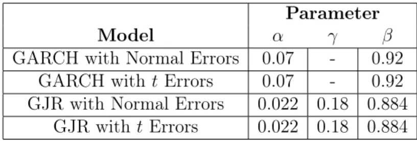
six in order to fatten the tails of the asset return process. In order to ensure comparability across models within our simulation, we change! so that the unconditional volatility of all the processes is 15 percent annually. Table 1 summarizes our parametrization.
Table 1: Parameterizations for Simulated-Asset Processes
Parameter Model ↵
GARCH with Normal Errors 0.07 - 0.92
GARCH with t Errors 0.07 - 0.92
GJR with Normal Errors 0.022 0.18 0.884 GJR witht Errors 0.022 0.18 0.884
Notes: The table provides parameter values for the volatility models used to generate the leverage multiplier in discrete time environments. We assume assets follow each of the four volatility models in the table above and we then simulate the leverage multiplier according to each parametrization.
For each process, we simulate the asset process 10,000 times from an initial asset value of
A0 = 1. We assume the debt matures in two years and, for simplicity, set the risk-free rate to
zero. The simulation generates a set of terminal values,AT, which in turn generate an equity
value for each value of debtD.13 We then compute numerical derivatives to measure how the
equity value changes with respect toA0. Finally, we calculate the leverage multiplier implied
by each asset return process and plot it against the implied financial leverage in Figure 4. The economics behind the shape of the leverage multiplier under various asset return processes are subtle. The benchmark case of BSM is given by the blue line in Figure 4, and it is easy to see that in a symmetric setting, making the tails of the asset distribution longer via GARCH decreases the leverage multiplier for larger values of debt (the green and red lines). For larger values of debt, extending the tails of the asset distribution serves the same function as increasing volatility in the BSM case. When we introduce asset volatility asymmetry via the GJR process, the leverage multiplier increases dramatically relative to the BSM benchmark (turquoise and purple lines). Volatility asymmetry effectively makes the figure asset distribution left skewed, which shortens the right tail of the distribution and
13E= 1
10,000
P10,000
i=1 max(AT,i D,0), whereiis the index for each simulation run. VaryingDgenerates
Figure 4: Simulated Leverage Multiplier in Stochastic Volatility and Non-Normality 0 5 10 15 20 25 30 35 40 45 50 0 5 10 15 De bt t o E q uit y Le v e r a g e M u lt ip li e r B S M G ARC H-N G ARC H-t G J R-N G J R-t
Notes: The figure plots the simulated leverage multiplier under different asset return process specifications. We consider GARCH and GJR process, each with normally distributed and t distributed errors. The unconditional volatility in all the models is 15 percent annually, the time to maturity of the debt is two years, and the risk-free rate is set to zero. The parameters of each volatility model can be found in Table1.
increases the leverage multiplier. In this case, leverage has a larger amplification on equity volatility because high leverage corresponds to a much smaller likelihood the equity expires “in the money.”
2.2.4. Three Properties of the Leverage Multiplier
In general, it is clear that the shape of the leverage multiplier is robust across a variety of continuous time and discrete time option pricing models. More specifically, our preceding analysis implies that the leverage multiplier satisfies at least three basic properties: (i) when leverage is zero, the leverage multiplier has a value of one, (ii) the leverage multiplier is weakly increasing in leverage, and (iii) the leverage multiplier is concave in leverage.
As previously discussed, the first property is mechanical and true by definition. It is slightly easier to prove the latter two properties within a specific option pricing framework, though it has proven more difficult to do so in a general setting. However, because we have shown that the leverage multiplier satisfies these three properties in a number of different option pricing models, we believe these three properties are not model dependent and likely derive from no arbitrage arguments. Perhaps more mildly, these properties should apply to asset processes whose distributions are plausible in the real world (that is, not a degenerative risk-neutral distribution with all the mass at some extreme point) and for reasonable levels of leverage. The remainder of our analysis will take these three properties as given. With this in mind, we propose a parameterized function to capture leverage amplification mechanisms in a relatively “model-free” way.
2.3. A Flexible Leverage Multiplier
In the derivation of Equation (9), we did not assign specific functions to g(·) and t. We
definegBSM(·)and BSM
t as the BSM inverse call and delta functions. We then propose the
following specification for the leverage multiplier:
LM⇣Dt/Et, A,tf ,⌧, rt; ⌘ = BSM t ⇣ Et/Dt,1, A,tf ,⌧, rt ⌘ ⇥gBSM⇣Et/Dt,1, fA,t,⌧, rt ⌘ ⇥ Dt Et (10) In this case, is the departure from the BSM model. When taking our model to data, it will be an estimated parameter. One advantage of our proposed leverage multiplier in Equation (10) is its relative simplicity in terms of computation, as the BSM delta and inverse call functions are numerically tractable. We discuss these potential computation issues later in Section3.2.
Figure 5: Leverage Multiplier for Different Values 0 5 10 15 20 25 30 35 40 45 50 1 2 3 4 5 6 7 8 9 10 11 De bt t o E q uit y Le v e r a g e M u lt ip li e r φ= 0.5 φ= 1 φ= 1.5
Notes: This figure plots the leverage multiplier according to the specification in (10) for different values of . In our baseline case, the annualized A is held constant at0.15,⌧ = 5, andr= 0.03.
It is worth emphasizing that our leverage multiplier simply uses a mathematical transfor-mation of the BSM functions. For example, in a BSM world, gBSM(·) would be interpreted
as the asset-to-debt ratio, but for our model it is simply a function. Similarly, BSM
t in our
specification is not interpreted as the correct hedge ratio, but merely serves as a function for our purposes. Let us now examine how our leverage multiplier changes for different values of , which we plot in Figure 5.
Unsurprisingly, increasing increases the leverage multiplier. For firms with a low value of , high levels of leverage have a small amplification effect in terms of equity volatility. Building on the intuition from the BSM case, we see that for these firms leverage plays a small role in the moneyness of the equity, which likely corresponds to healthier firms. The converse holds true as well, as firms with high experience large equity volatility amplification, even
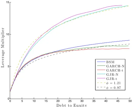
Figure 6: Simulated Leverage Multiplier and Our Specification 0 5 10 15 20 25 30 35 40 45 50 0 5 10 15 De bt t o E q uit y Le v e r a g e M u lt ip li e r B S M G ARC H-N G ARC H-t G J R-N G J R-t φ= 1.21 φ= 0.97
Notes: The figure plots the simulated leverage multiplier under different asset return process specifications. We consider GARCH and GJR process, each with normally distributed and t distributed errors. The unconditional volatility in all the models is 15 percent annually, the time to maturity of the debt is two years, and the risk-free rate is set to zero. The parameters of each volatility model can be found in Table1. In addition, we plot our leverage multiplier from specification (10) for different values of to demonstrate that our model captures various asset return processes well.
for low levels of financial leverage.
To highlight the flexibility of our specification, we revisit the Monte Carlo exercise from Section 2.2.3. Figure 6plots the leverage multiplier in a GARCH option pricing setting, as well as our leverage multiplier for a few different values of .
Figure 6 shows that varying in our leverage multiplier specification captures various asset return processes well. Increasing is successful in matching the patterns in the leverage multiplier that arise in stochastic volatility, asymmetric volatility, and non-normal settings. Importantly, our flexible leverage multiplier also preserves the three necessary properties outlined in Section2.2.4. Raising the BSM leverage multiplier to an arbitrary power naturally
preserves the condition forLM(·)to have a value of one when leverage is zero. It is also clear
from Figure 5and Figure 6 that varying preserves the concavity and increasing nature of the BSM leverage multiplier.14 While our specification is seemingly simple, it is not a trivial
task to define a function that retains the flexibility of ours but also maintains the necessary properties of the leverage multiplier. Our analysis in Section 2.2.1 also demonstrated that
LM is decreasing in asset volatility and time-to-maturity.15 Because our leverage multiplier
is a power function of the BSM multiplier, an additional advantage of our specification is that it inherits these natural properties from the Black-Scholes-Merton model.
2.4. The Full Recursive Model
The preceding analysis motivates the use of our leverage multiplier in describing the relation-ship between equity volatility and leverage. To make the model fully operational in discrete time, we propose the following process for equity returns:
rE,t = LMt 1rA,t
rA,t =
p
hA,t"A,t, "A,t⇠D(0,1)
hA,t = !+↵ ✓ rE,t 1 LMt 2 ◆2 + ✓ rE,t 1 LMt 2 ◆2 1rE,t 1<0+ hA,t 1 LMt 1 = 4BSMt 1 ⇥gBSM ⇣ Et 1/Dt 1,1, fA,t 1,⌧ ⌘ ⇥ DEt 1 t 1 (11)
14To be precise, preserves the concavity so long as it is not too large, long-run asset volatility is not too small, and ⌧ is not too small. In practice, this is not an issue, even for financial firms who have larger
amounts of leverage. When we estimate the model, we later verify that none of the fitted result in violations of this sort.
15Our analysis in Section2.2.1applied to the BSM model, but the notion that the leverage multiplier is decreasing in both asset volatility and time to maturity holds more broadly. Merton (1974) shows that as the time-to-maturity goes to infinity, the option becomes the same as the underlying, so the leverage multiplier must decrease to its lower bound of one (Theorem 3). Similarly, the call option pricing formula is weakly increasing in volatility (Theorem 8). So long as the rate of increase in the delta of the option w.r.t volatility
We will call the specification described in Equation (11) as a “Structural GARCH” model.16
The parameter set for the Structural GARCH is⇥:= (!,↵, , , ), so there is only one extra
parameter compared to a vanilla GJR model. We will confront the issue of how to compute ⌧ and fA,t 1 in the next section when describing the data and estimation techniques used in our empirical work. We also introduce lags in the appropriate variables (e.g., the leverage multiplier) to ensure that one-step ahead volatility forecasts are indeed in the previous day’s information set. The model in (11) nests both a simple GJR model ( = 0) and the BSM
model ( = 1), and provides a statistical test of how leverage affects equity volatility.17 This
is another attractive feature of our leverage multiplier from an econometric perspective, and adds to the theoretically appealing qualities we highlighted in Section 2.3.
The equity return series will inherit volatility asymmetry from the asset return series, an important feature of equity returns in the data.18 The recursion for equity returns (and
asset returns) in (11) is simple and straightforward to compute, yet powerful. For example, when simulating this model, if a series of negative asset returns is realized (and hence nega-tive equity returns since they share the same shock), volatility rises due to the asymmetric specification inherent in the GJR. In that case, leverage also rises, increasing the leverage multiplier and resulting in an even stronger amplification effect for equity volatility. As we 16In reality our model is a Structural GARCH(1,1) model, because it includes a single lag of the squared asset return and asset volatility. Incorporating a richer lag structure is straightforward, so that our model can naturally be generalized to Structural GARCH(p, q)model as follows:
hA,t=!+ p X j=1 ↵j ✓ rE,t j LMt j 1 ◆2 + p X j=1 j ✓ rE,t j LMt j 1 ◆2 1rE,t j<0+ q X i=1 ihA,t i
17 = 1 nests the BSM exactly if we use a constant forecast of asset volatility over the lifetime of the option. As mentioned, we estimate this model against a model where we use a GJR forecast for f
A,t. The results are similar, so we refer to the two without distinction.
18For example, it is has been shown that a GJR process for equity can replicate features of equity option data like the volatility smirk.
saw in the recent financial crisis, this was a key feature of the data, particularly for highly leverage financial firms. Additionally, by letting vary from firm-to-firm, we effectively allow a different option pricing model to apply to the capital structure of each firm. This flexibility is difficult to achieve if we impose an option pricing model on the data a priori because, as we showed, allows us to move across differentclasses of option pricing models. To the extent that our leverage multiplier form captures various option pricing models, the Structural GARCH allows us to infer a high frequency asset return series with stochastic volatility in a relatively model-free way. Later, this will prove to be extremely useful for a number of applications of the model.
We also wish to emphasize there are many ways to parameterize the observation that the leverage multiplier is similar across option pricing models for the purposes of volatility mod-eling. We have chosen a particular specification that balances parsimony with the underlying economics, while still retaining useful statistical properties. However, the themes that under-lie the Structural GARCH are broader than our specific econometric model. An additional contribution of this paper is to provide a simple and economically grounded framework with widespread application for modeling volatility and leverage jointly.
3. Data Description and Estimation Details
3.1. Data Description
We now turn to estimating the Structural GARCH model using equity return data. To compute the leverage multiplier, we also need balance sheet information. Unless otherwise noted, we obtain all of our data from Bloomberg. In particular, we define Dt as the book
value of debt at timet.19 To avoid estimation issues inherent with quarterly data, we smooth
the book value of debt using an exponential average with smoothing parameter of 0.01. This smoothing parameter value implies a half-life of approximately 70 days in terms of the weights of the exponential average, which is reasonable for quarterly data.
The set of firms we analyze are financial firms over a period that spans from January 3, 1990 to February 14, 2014.20 The reasons we focus on financial firms are twofold: first, these
firms typically have extraordinarily high leverage and structural models have failed to model these firms well. Second, given the high volatility in the recent crisis that was accompanied by unprecedented leverage, this set of firms presents an important sector to model from a systemic risk and policy perspective. To this end, one of the applications of our model that we will explore in later sections involves systemic risk measurement of financials. In future work, we hope to extend the set of firms we analyze.
3.2. Numerical Implementation
When estimating the full model, we use quasi-maximum likelihood and the associated stan-dard errors for parameter estimates. In order to ensure a global optimum is reached, we also conduct each maximum likelihood optimization over a grid of 24 different starting val-ues.21 Despite the relative simplicity of our model, quasi-maximum likelihood estimation is
still quite costly from a computational perspective. To see why, let us explicitly define our 19All liabilities are treated as exogenous and as if they have a single expiration. Liabilities are measured as the book value of assets minus the book value of equity from quarterly accounting statements. Some models use maturity measures directly however for financial firms many of the liabilities do not have contractual liabilities. We discuss the issue of debt maturity below.
20A full description of the set of firms is contained in AppendixD.1.
21The Matlab code for estimation of the model via quasi-maximum likelihood (QMLE) with the correct standard errors is available upon request.
log-likelihood function from the specification in (11): L⇣!,↵, , , ;{rE,t, Et, Dt}Tt=2 ⌘ := 1 2 T X t=2 "
log(2⇡) + log(hE,t) +
(rE,t)2 hE,t # = 1 2 T X t=2 "
log(2⇡) + log(LMt2 1hA,t) +
(rE,t)2
LM2
t 1hA,t #
where all summations begin from t = 2 because the leverage multiplier contains lagged
equity and debt values. From our definition of the leverage multiplier, it is clear that a single computation of LMt requires an inversion of the BSM call option formula. For a firm with
10 years of data, this means evaluating L(·)at a single parameter set requires approximately 10⇥252 = 2520inversions of the BSM call option formula. In turn, maximizing a single firm’s
likelihood function typically involves 180 function evaluations, which means 2520⇥180 = 453,600 inversions. As mentioned, we use 24 different starting values to ensure a global
maximum is reached, two different types of asset volatility over the life of the debt, and 30 different debt maturities (more details follow). In total, this means for an average firm in our sample, we must invert the BSM function 2520⇥280⇥24⇥2⇥30 = 1,016,064,000 times,
which is computationally expensive given there is no closed form formula for the inverse BSM function.22
To make the problem computational tractable, we estimate all of our models on the Amazon Elastic Compute Cloud. The computing unit we use is their latest generation Linux based machine with 32 CPUs, and 60 GB of RAM. Estimation of each firm is done using parallel processing, and the average firm takes about 80 minutes to estimate the full model. Since we estimate the model for more than 80 firms, we use many different computing 22Later in Section6, we will simulate the Structural GARCH models thousands of times over long horizons, also a computationally taxing task for similar reasons.
units simultaneously to make the total time more reasonable (approximately 12 hours for all firms).
The remaining issues are how to treat both the time to maturity of the debt ⌧, the asset volatility over the life of the debt f
A,t, and the risk-free rate, rt.
Time to Maturity of the Debt
An input to the leverage multiplier is time to maturity of the debt. Because the book value of debt combines a number of different debt maturities, we simply iterate over different ⌧ during estimation. Specifically, we estimate the model for ⌧ 2 [1,30], restricting ⌧ to take on integer values. We keep the version of the model that attains the highest log-likelihood function.
Risk Free Rate
To compute the leverage multiplier, we must also input the risk free rate over the life of the debt. We do so by using a zero-curve provided by OptionsMetrics, which is derived from BBA LIBOR rates and settlement prices of CME Eurodollar futures. We then linearly interpolate (with flat endpoints beyond the maximum maturity) to determine the riskless rate for a specific maturity.
Asset Volatility Over Life of Debt
We take two different approaches for the computing the value of f
A,t. The first is to
use the unconditional volatility implied by the asset volatility series corresponding to the unconditional volatility of a GJR process. Using a constant f
A,tin fact completely eliminates
any issues in ignoring the vega terms in our motivating derivation of the leverage multiplier (see Equation (3)). The second approach is to use the GJR forecast over the life of the debt
at each date t. It is straightforward to derive the closed form expression for this forecast.
We use both approaches for f
A,t and choose the model with the highest likelihood.
4. Empirical Results
4.1. Cross-Sectional Summary
We begin by presenting a cross-sectional summary of the estimation results.23 Since the main
contribution of this paper is the leverage multiplier, Figure7plots the estimated time-series of the lower quartile, median, and upper quartile leverage multipliers, across all firms.
As we can see, there is considerable cross-sectional heterogeneity in the leverage multi-plier, even within financial firms. It appears that across all firms, the leverage multiplier moves with the business cycle, which is not surprising given that leverage itself tends to do so as well. In the top quartile of firms, leverage amplified equity volatility by a factor of eight during the financial crisis. Evidently, for this set of firms, the leverage amplification mechanism has remained high in the years following the crisis.
Table 1shows cross-sectional summary statistics for the point estimates of the Structural GARCH model. In our model, the first four estimates represent the GJR parameters for the asset return series. It is not surprising then that they resemble those found in equity returns. The parameter ! is an order of magnitude smaller than usual, but this is natural because asset returns are less volatile than equity returns and! is a determinant of the unconditional volatility. The asset process is indeed stationary, as seen by the combination of ↵, , and
23There were 11 firms where the estimated coefficient had convergence issues and hit the lower bound for . We discuss these firms specifically in AppendixD.2. The main unifying theme with these firms is that their leverage is both low and nearly constant through the time series, so identification of is difficult. We exclude these firms for the remainder of the analysis.
Figure 7: Time Series of Leverage Multiplier Across Quartiles 19971 2000 2002 2005 2007 2010 2012 2015 2 3 4 5 6 7 D at e Le v e r a g e M u lt ip li e r Me d i a n L M L o w e r Q u a r t i l e L M U p p e r Q u a r t i l e L M
Notes: The figure plots the quartiles of the estimated leverage multiplier across firms, and through time. The plot begins in January 1998 and ends in February 2014. The full set of firms we analyze can be found in AppendixD.1
standard results on the stationarity of GARCH processes. One subtle but key difference in the current estimates is the parameter , which is higher than it is for equity returns in this subset of stocks. Recall that dictates the correlation between volatility and returns, and thus it appears that the volatility asymmetry we observe in equity is somewhat dampened in asset returns. In one application of the model, we will explore this idea further as it pertains to the classical leverage effect of Black(1976) and Christie(1982).
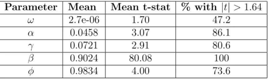
The new parameter in our model is . The third and fourth columns of Table 2 show is statistically different than zero for a majority of firms. Therefore, the effect of leverage on
Table 2: Cross-Sectional Summary of Structural GARCH Parameter Estimates
Parameter Mean Mean t-stat % with |t|>1.64
! 2.7e-06 1.70 47.2
↵ 0.0458 3.07 86.1
0.0721 2.91 80.6
0.9024 80.08 100
0.9834 4.00 73.6
Notes: This table provides a cross-sectional summary of the parameter estimates from the Structural GARCH model as defined in Equation (11). The full set of firms we analyze can be found in AppendixD.1.
equity volatility via our leverage multiplier appears to be substantial for a large number of financial firms. Interestingly, the average is slightly less than one, as the BSM model would suggest. These results are roughly consistent with the findings of Schaefer and Strebulaev
(2008) who find that while the Merton (1974) model does poorly in predicting the levels of credit spreads, it is successful in generating the correct hedge ratios across the capital structure of the firm. In our context, we interpret their finding and our estimation of to mean that the Merton model does well in recovering the daily returns of assets well, even if it is not able to pinpoint the level of assets.
4.2. Aggregation
4.2.1. Aggregate Leverage Multiplier
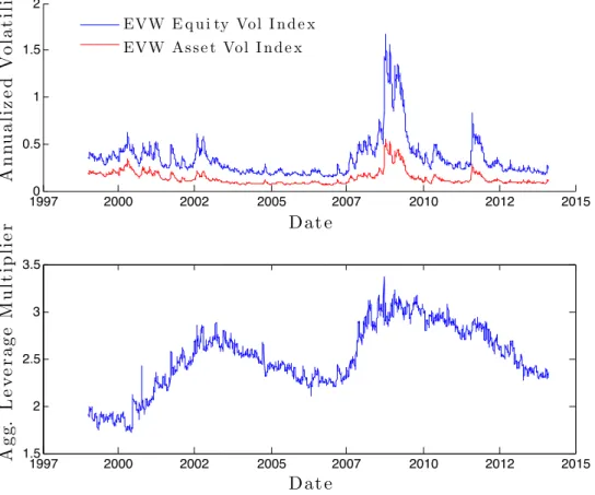
We aggregate our results across firm by creating three indices: 1) a value-weighted average equity volatility index, 2) a value-weighted average asset volatility index, and 3) an aggregate leverage multiplier. The aggregate leverage multiplier is simply the ratio of the equity volatility index to the asset volatility index. The weights used in creating each respective index are derived from equity valuations. Figure 8 plots these three time series. Again, it
Figure 8: Aggregate Equity Volatility, Asset Volatility, and Leverage Multiplier 19970 2000 2002 2005 2007 2010 2012 2015 0.5 1 1.5 2 D at e An n u a li z e d V o la t il it y EVW E q u i ty Vol I n d e x EVW As s e t Vol I n d e x 1997 2000 2002 2005 2007 2010 2012 2015 1.5 2 2.5 3 3.5 D at e A g g. L e v e r a g e M u lt ip li e r
Notes: This figure plots the value-weighted average across all firms of our estimated equity volatility and asset volatility. The weights used in creating each respective index are based on equity valuations. The aggregate leverage multiplier is then the ratio of the aggregate equity volatility index to the asset volatility index.
is clear that there is a cyclicality in the aggregated leverage multiplier. A pressing issue in the wake of the financial crisis is the role of leverage and the health of the financial sector. Since our model provides estimates of leverage amplification in terms of equity volatility (as well as asset volatility), we focus on these aggregated time-series through the financial crisis in Figure 9.
Figure 9: Aggregate Equity Volatility, Asset Volatility, and Leverage Multiplier During Financial Crisis 20070 2008 2009 2010 0.5 1 1.5 2 D at e An n u a li z e d V o la t il it y E VW E q u i t y Vol I n d e x E VW As s e t Vol I n d e x 20072 2008 2009 2010 2.5 3 3.5 D at e A g g. L e v e r a g e M u lt ip li e r
Notes: This figure plots the value-weighted average across all firms of our estimated equity volatility and asset volatility. The weights used in creating each respective index are based on equity valuations. The aggregate leverage multiplier is then the ratio of the aggregate equity volatility index to the asset volatility index. Our time period focuses on the financial crisis from 2007 to mid-2009.
summer of 2007. However the rise in asset volatility did not really occur until late in 2008. The increase in leverage in 2007 was partly an increase in aggregate liabilities and partly a fall in equity valuation. After the fall of Lehman Brothers Holdings, Inc., asset volatility rose dramatically as well and the leverage multiplier continued to rise before stabilizing in the spring of 2009.
5. The Leverage E
ff
ect
We now turn to our first application of the Structural GARCH: the leverage effect. The leverage effect ofBlack (1976) and Christie (1982) documents the negative correlation that exists between equity returns and equity volatility. One possible explanation for this fact is that when a firm experiences a fall in equity, its financial leverage mechanically rises, the company becomes riskier, and volatility rises.
A second explanation points to the role of risk premiums in describing the negative cor-relation between equity returns and equity volatility (e.g. French, Schwert, and Stambaugh
(1987)). In this explanation, a rise in future volatility raises the required return on equity, leading to an immediate decline in the stock price. The Structural GARCH model provides a natural framework to explore these issues econometrically.24
Recall that the Structural GARCH model delivers an estimate of the daily return of assets.25 Any correlation between asset volatility and asset returns can not be due to financial
leverage. So, if a correlation does exist, it must be attributed to a risk-premium argument. When applying the GJR volatility model to a given time series of returns, the parameter is one way to measure the correlation between the volatility and returns (e.g. a higher corresponds to more negative correlation). Therefore, we would expect the GJR estimated from equity returns to be larger than the same parameter estimated from asset returns. Indeed, the median for equity returns is 0.0811 and the median for asset returns is 24Other econometric studies of the leverage effect includeBekaert and Wu(2000). The difference in our approach is that we allow debt for the firm to be risky, as in theMerton(1974) model.
25Again, this relies on a few assumptions. First, our specification ignores the effect of changes in long-run asset volatility on daily equity returns. Second, we assume that the book value of debt adequately captures the outstanding liabilities of the firm. For example, we do not consider non-debt liabilities in our baseline specification. Still, the Structural GARCH model is, at worst, effective in at least partially unlevering the firm.
0.0676. For our subsample of firms, financial leverage accounts for roughly 17 percent of the leverage effect.
To put a bit more structure on the implications of Structural GARCH and the leverage effect, we run the following cross-sectional regression:
E,i A,i =a+b⇥D/Ei+errori (12)
where E,i and A,i are the estimated GJR asymmetry parameter for firm i’s equity returns
and firm i’s asset returns respectively. D/Ei is the mean debt to equity ratio for firm i
over the sample period. The logic behind the regression in (12) is simple — to the extent that leverage contributes to equity volatility asymmetry, firms with higher leverage should experience a larger reduction in volatility asymmetry after unlevering the firm. Table 3 presents the results.
Table 3: Equity Asymmetry versus Asset Asymmetry
Variable Coefficient Value t-stat R2
b 0.0016 3.18 13.04%
Notes: This table presents the cross-sectional regression described in Equation (12). We regress the difference between the asymmetric volatility coefficient for equity and assets( E,i A,i)on the mean of the debt to equity ratio for each firm in our sample.
As expected, firms with higher average leverage have a larger gap between their equity and asset asymmetry. As we saw before, there is still a substantial amount of asset volatility asymmetry (the median parameter for assets is 0.0676), which is helps explain why the
R2 is not higher. At the asset level, firms with higher volatility asymmetry should have
regression:
Stage 1: rA
i,t =c+ mkt,iA rmkt,tE +ei,t
Stage 2: A,i =e+f⇥ mkt,iA +"i (13)
where rE
mkt is the return on the equity market index. Stage 1 of the regression is designed
to deliver a measure of firms’s risk premium through its CAPM beta.26 The coefficientf in
the Stage 2 regression is the main variable of interest. A positive value corroborates the risk premium story for volatility asymmetry. The results of the two-stage regression are found in Table 4.
Table 4: Risk-Premium Effect on Asset Asymmetry
Variable Coefficient Value t-stat R2
f 0.0190 1.35 2.62%
Notes: This table presents the two-stage regression results in Equation (13). The first stage regression estimates, for each firm’s asset return series, the equity market beta. The second stage regresses a measure of asset volatility asymmetry, the GJR asset , on the regression coefficient from Stage 1.
Unsurprisingly, firms with higher market betas have higher asset volatility asymmetry. Though the results are weak, we view them as qualitative confirmation for how the Structural GARCH unlevers the firm. Part of the reason for the standard error of our estimate of f is
that we compute A
mkt,i at the firm level, and it is well known that betas are more precisely
measured at the portfolio level. In addition, Bekaert and Wu (2000) attribute a portion of firm-level volatility asymmetry to covariance asymmetry between the market and the firm’s equity. Our cross-sectional investigation does not include this (or other) potential
26Note that since we are interested in the cross-sectional behavior of
A,iwe are not concerned with using the return on the equity market. If, for example, we used some proxy for a broad market asset market index, only the magnitude of the coefficientf would change.
explanations, and is outside the scope of this paper. We now turn to using the Structural GARCH model to measure systemic risk.
6. Systemic Risk Measurement
Given the unprecedented rise in leverage and equity volatility during the financial crisis of 2007-09, systemic risk measurement is a natural application of the Structural GARCH model. Consider the following thought experiment: Following a negative shock to equity value, the financial leverage of the firm mechanically rises. In a simple asymmetric GARCH model for equity, the rise in volatility following a negative equity return is invariant to the capital structure of the firm. However, in the Structural GARCH model, the leverage multiplier will be higher following a negative equity return. Thus, equity volatility will be more sensitive to even slight rises in asset volatility. In simulating the model, this mechanism would manifest itself if the firm experiences a sequence of negative asset shocks. Due to asset volatility asymmetry, a sequence of negative asset returns increases asset volatility. In turn, there may potentially be explosive equity volatility since the leverage multiplier will be large in this case. Casual observation of equity volatility and leverage during the crisis clearly supports such a sequence of events.
6.1. Traditional SRISK
In order to embed this appealing feature of the Structural GARCH model into systemic risk measurement, we adapt the SRISK metric ofBrownlees and Engle(2012) andAcharya, Pedersen, Philippon, and Richardson (2012). The reader should refer to these studies for an in-depth discussion of SRISK, but we will provide a brief summary here. Qualitatively,
SRISK is an estimate of the amount of capital that an institution would need in order to function normally in the event of another financial crisis. To compute SRISK, we first compute a firm’s marginal expected shortfall (MES), which is the expected loss of a firm when the overall market declines a given amount over a given time horizon.27 In turn, MES
requires us to simulate a bivariate process for the firm’s equity return, denoted rE
i,t, and the
market’s equity return, denotedrE
m,t. The bivariate process we adopt is described as follows:
rm,tE = qhE m,t"m,t ri,tE = q hE i,t ⇣ ⇢i,t"M,t+ q 1 ⇢2 i,t⇠i,t ⌘ = LMi,t 1 q hA i,t ⇣ ⇢i,t"M,t+ q 1 ⇢2 i,t⇠i,t ⌘ ("m,t,⇠i,t) ⇠ F (14)
where the shocks ("m,t,⇠i,t) are independent and identically distributed over time and have
zero mean, unit variance, and zero covariance. We do not assume the two shocks are in-dependent, however, and allow them to have extreme tail dependence nonparametrically.28
The processes hE
m,t, hEi,t and ⇢i,t represent the conditional variance of the market, the
condi-tional variance of the firm, and the condicondi-tional correlation between the market and the firm, respectively. It is important to note that under the Structural GARCH model, we are really estimating correlations between shocks to the equity market index and shocks to firm asset returns. Generically, once the bivariate process in (14) is fully specified, we compute a six month MES (henceforth LRMES for “long-run” marginal expected shortfall) by simulating the joint processes for the firm and the market (with bootstrapped shocks) and conditioning 27Acharya, Pedersen, Philippon, and Richardson(2012) provide an economic justification for why marginal expected shortfall is the proper measure of systemic risk in the banking system.
on the event that the market declines by 40 percent. Incorporating the Structural GARCH model into LRMES is simple. As stated in Equation (14), we simply assume the volatility process for firm equity returns follows a Structural GARCH model.29 Finally, we assume
that equity market volatility follows a familiar GJR(1,1) process and that correlations follow a DCC(1,1) model.
Once we have an estimate for the LRMES of a firm on a given day, we compute its capital shortfall in a crisis as follows:
CSi,t =kDebti,t (1 k)(1 LRM ESi,t)Ei,t (15)
where Debti,t is the book value of debt outstanding on the firm, Ei,t is the market value of
equity, and k is a prudential level of equity relative to assets. In our applications, we take k = 8 percent and, as is conventional in risk metrics such as VaR, we use positive values
of LRM ESi,t to represent declines in the firm’s value. For example, if firmi is expected to
lose 60 percent of its equity in a crisis, its LRMES will be 60percent. Thus, positive values
of capital shortfall mean the firm will be short of capital in a crisis. Finally, we define the SRISK of a firm as:
SRISKi,t = max(CSi,t,0)
The parameters governing the market volatility and firm-market correlation are estimated recursively and allowed to change daily. However, due to the computational burden of estimating the Structural GARCH recursively each day, we use the full sample to estimate the Structural GARCH parameters. In future versions of SRISK measurement with Structural 29Efficient simulation of a bivariate Structural GARCH process is, however, not trivial. The MATLAB© code for this purpose is available from the authors upon request. All parameters of the model are estimated using our full sample of data for each firm.
GARCH, we hope to estimate all parameters of the bivariate process recursively. In the interest of brevity, we choose to focus on one firm: Bank of America.
To start, Figure 10plots the LRM ES for Bank of America under using both the
Struc-tural GARCH, as well as a vanilla GJR model of univariate returns. Figure 10: LRM ES for Bank of America
Notes: The figure above plots the Long Run Marginal Expected Shortfall (LRMES) of Bank of America. The purple line is the LRMES using a standard GJR model for returns. The orange line is the same calculation using the Structural GARCH model. The sample period is from January 2000 to November 2011.
It is obvious that the Structural GARCH induces a higher MES than a standard asym-metric volatility model. The reasons for this pattern are due to the leverage amplification mechanism built into the model directly. In the low-volatility period from 2004-2007, the Structural GARCH model delivers a LRM ES nearly double the value that comes from a
Structural GARCH model that result in increases in leverage, which in turn result in higher volatility, and therefore paths where equity suffers large losses. There is much less of a scope for this type of leverage spiral in low volatility/leverage periods in our typical volatility mod-els. To focus in on the recent financial crisis, we translate our LRM ES calculations into
SRISK and plot the resulting series from starting in 2007 in Figure 11.
Figure 11: SRISK for Bank of America
Notes: The figure above plots theSRISKof Bank of America from November 2006 to November 2011. The units of they-axis are millions of USD. The blue line uses a standard GJR model for returns. The green line is the same calculation using the Structural GARCH model.
Figure 11 illustrates why the Structural GARCH model may provide useful in terms of providing early warning signals of threats to financial stability. The results echo the dynamics
early as January 2007, the SRISK (using Structural GARCH) of Bank of America starts to rise and hovers around $20 billion. On the other hand, SRISK derived from a standard asymmetric volatility model shows no (expected) capital shortfalls until late 2007 and early 2008. Again, the success of the Structural GARCH along this dimension rests with the inherent leverage-volatility connection within the model. Qualitatively, the volatility and leverage link is apparent and has been discussed extensively in the media and the academic literature. Quantitatively, this link has been hard to pin down. The results in Figure 11 are evidence that the Structural GARCH model is, at very least, a partial resolution of this issue.
6.2. Structural GARCH and the Probability of Default
While the SRISK framework provides a way to assess the capital deficiencies of financial firms in a crisis, an alternative way to explore this issue is to ask the following: how likely is a firm to go bankrupt if crisis occurs? To answer this question, we use the same simulation machinery as in our SRISK analysis. Namely, for a given date, we condition on the market falling 40 percent over six months, and then we simulate future return paths of the firm using the bivariate specification in (14). We then compute the (conditional) probability of a firm going bankrupt as the proportion of simulated paths where bankruptcy occurs (i.e. when equity valuation hits zero). Our simulations again use two competing volatility models for returns: (i) the Structural GARCH and (ii) a standard GJR volatility model. For the purpose of illustration, we conduct this analysis for Bank of America on August 29, 2008.
Table 5 contains statistics on Bank of America’s bankruptcy paths over various horizons and under both models. The connection between volatility and leverage is clearly seen in this setting as well, as the likelihood of Bank of America going bankrupt is five times higher under
Table 5: Conditional Probability of Default
Structural GARCH Regular GJR Total # of Paths 453 453
# of Bankruptcies 45 9
Probability of Bankruptcy 9.93% 1.99%
Avg. Time to Bankruptcy 89.4 91.2
Min Time to Bankruptcy 42 57
Max Time to Bankruptcy 126 126
Notes: This table contains basic summary statistics for Bank of America’s simulated bankruptcy paths starting from August 29, 2008. The simulations are: (i) over a six month horizon; (ii) conducted using the Structural GARCH and a GJR model; (iii) and are conditional on a drop of 40 percent in the aggregate market over the same timeframe. The number of simulations is 1841.
the Structural GARCH model relative to the GJR model. At the end of August 2008, the Structural GARCH model indicated that Bank of America had a nearly 10 percent chance of going bankrupt should a crisis occur over the next six months, whereas the GJR model suggests only a 2 percent chance of this outcome. This is because the GJR model cannot hope to capture how leverage increases the future risk of the firm and makes bankruptcy more likely as the firm’s leverage explodes. In addition, the minimum time to bankruptcy and the average time to bankruptcy are shorter in the Structural GARCH model, which is another way of depicting the type of volatility-leverage spirals our model is designed to encompass.
6.3. A New Measure of Systemic Risk: Precautionary Capital
Based on our preceding analysis of SRISK, it is clear that accounting for the interaction between volatility and leverage is extremely important. Our model provides a simple way to capture the nonlinear way in which increasing leverage increases current and future risk to equity holders, and vice versa. SRISK in one sense asks how much trouble would a financial