Efficient And Effective Model Order Reduction Algorithms

A

M

C M

Bergische Universit¨

at Wuppertal

Fachbereich Mathematik und Naturwissenschaften

Institute of Mathematical Modelling, Analysis and

Computational Mathematics (IMACM)

Preprint BUW-IMACM 15/11

A.C. Antoulas, R. Ionutiu, N. Martins, E.J.W. ter Maten,

K. Mohaghegh, R. Pulch, J. Rommes, M. Saadvandi, M. Striebel

Model Order Reduction

Methods, Concepts and Properties

February 2015

Chapter 3

Model Order Reduction — Methods, Concepts

and Properties

Athanasios C. Antoulas, Roxana Ionutiu, Nelson Martins, E. Jan W. ter Maten, Kasra Mohaghegh, Roland Pulch, Joost Rommes, Maryam Saadvandi and Michael Striebel

Athanasios C. Antoulas

William Marsh Rice University, Department of Electrical and Computer Engineering, MS-380, PO Box 1892, Houston, TX, 77251-1892, USA, e-mail:[email protected],

and

School of Engineering and Science, Jacobs University Bremen, 28725 Bremen, Germany, e-mail: [email protected].

Roxana Ionutiu

ABB Switzerland Ltd, ATTE, Austraße, 5300 Turgi, Switzerland, e-mail:Roxana.Ionutiu@ ch.abb.com.

Nelson Martins

CEPEL, 21941-911, Rio de Janeiro, RJ, Brazil, e-mail:[email protected]. E. Jan W. ter Maten

Chair of Applied Mathematics/Numerical Analysis, Bergische Universit¨at Wuppertal, Gaußstraße 20, D-42119 Wuppertal, Germany, e-mail:[email protected], and

Eindhoven University of Technology, Department of Mathematics and Computer Science, CASA, P.O.Box 513, 5600 MB Eindhoven, the Netherlands, e-mail:[email protected]. Kasra Mohaghegh

Multiscale in Mechanical and Biological Engineering (M2BE), Arag´on Institute of Engineering Research (I3A), University of Zaragoza, Mar´ıa de Luna, 3, E-50018, Zaragoza, Spain, e-mail: [email protected].

Roland Pulch

Institut f¨ur Mathematik und Informatik, Ernst Moritz Arndt Universit¨at Greifswald, Walther-Rathenau-Straße 47, D-17487 Greifswald, Germany, e-mail:[email protected]. Joost Rommes

NXP Semiconductors, HTC 60, 5656 AE Eindhoven, the Netherlands, e-mail:Joost.Rommes@ NXP.com.

Maryam Saadvandi

Numerical Approximation and Linear Algebra Group, Dept. of Computer Science, KU Leu-ven, Celestijnenlaan 200A, 3001 Heverlee, Belgium, e-mail: Maryam.Saadvandi@cs. kuleuven.be.

Michael Striebel

ZF Lenksysteme GmbH, Richard-Bullinger-Straße 77, D-73527 Schw¨abisch Gm¨und, Germany, e-mail:[email protected].

AbstractThis Chapter offers an introduction to Model Order Reduction (MOR). It gives an overview on the methods that are mostly used. It also describes the main concepts behind the methods and the properties that are aimed to be preserved. The Sections are in a prefered order for reading, but can be read independentlty. Sec-tion 3.1, written by Michael Striebel, E. Jan W. ter Maten, Kasra Mohaghegh and Roland Pulch, overviews the basic material for MOR and its use in circuit simu-lation. Issues like Stability, Passivity, Structure preservation, Realizability are dis-cussed. Projection based MOR methods inlude Krylov-space methods (like PRIMA and SPRIM) and POD-methods. Truncation based MOR includes Balanced Trunca-tion, Poor Man’s TBR and Modal Truncation.

Section 3.2, written by Joost Rommes and Nelson Martins, focuses on Modal Trun-cation. Here eigenvalues are the starting point. The eigenvalue problems related to large-scale dynamical systems are usually too large to be solved completely. The algorithms described in this section are efficient and effective methods for the com-putation of a few specific dominant eigenvalues of these large-scale systems. It is shown how these algorithms can be used for computing reduced-order models with modal approximation and Krylov-based methods.

Section 3.3, written by Maryam Saadvandi and Joost Rommes, concerns passivity preserving model order reduction using the spectral zero method. It detailedly dis-cusses two algorithms, one by Antoulas and one by Sorenson. These two approaches are based on a projection method by selecting spectral zeros of the original transfer function to produce a reduced transfer function that has the specified roots as its spectral zeros. The reduced model preserves passivity.

Section 3.4, written by Roxana Ionutiu, Joost Rommes and Athanasios C. Antoulas, refines the spectral zero MOR method to dominant spectral zeros. The new model reduction method for circuit simulation preserves passivity by interpolating domi-nant spectral zeros. These are computed as poles of an associated Hamiltonian sys-tem, using an iterative solver: the subspace accelerated dominant pole algorithm (SADPA). Based on a dominance criterion, SADPA finds relevant spectral zeros and the associated invariant subspaces, which are used to construct the passivity preserving projection. RLC netlist equivalents for the reduced models are provided. Section 3.5, written by Roxana Ionutiu and Joost Rommes, deals with synthesis of a reduced model: reformulate it as a netlist for a circuit. A framework for model reduction and synthesis is presented, which greatly enlarges the options for the re-use of reduced order models in circuit simulation by simulators of choice. Especially when model reduction exploits structure preservation, we show that using the model as a current-driven element is possible, and allows for synthesis without controlled sources. Two synthesis techniques are considered: (1) by means of realizing the reduced transfer function into a netlist and (2) by unstamping the reduced system matrices into a circuit representation. The presented framework serves as a basis for reduction of large parasitic R/RC/RCL networks.

Co-operations between the various co-authors

The subactivity on Model Order Reduction (MOR) of the COMSON project1_was

greatly influenced by interaction with additional research on MOR, first at Philips Research Laboratories and (from october 2006 on) at NXP Semiconductors (both in Eindhoven). There was direct project work with the TU Eindhoven, with the Bergische Universit¨at Wuppertal and with the Royal Institute of Technology (KTH) in Stockholm:

• R. IONUTIU: Model order reduction for multi-terminal Systems - with

appli-cations to circuit simulation. Ph.D.-Thesis, TU Eindhoven, 2011, http:// alexandria.tue.nl/extra2/716352.pdf.

• M. SAADVANDI:Passivity preserving model reduction and selection of

spec-tral zeros. MSc. Thesis, Royal Institute of Technology (KTH), Stockholm. Also published as Technical Note NXP-TN-2008/00276, Unclassified Report, NXP Semiconductors, Eindhoven, 2008. [In September 2012, Maryam Saadvandi did complete a Ph.D.-Thesis at KU Leuven, Belgium, onNonlinear and parametric model order reduction for second order dynamical systems by the dominant pole algorithm.]

• M.V. UGRYUMOVA: Applications of Model Order Reduction for IC Model-ing. Ph.D.-Thesis, TU Eindhoven, 2011,http://alexandria.tue.nl/ extra2/711015.pdf.

• A. VERHOEVEN:Redundancy reduction of IC models by multirate time-integra-tion and model order reductime-integra-tion. Ph.D.-Thesis, TU Eindhoven, 2008,

http://alexandria.tue.nl/extra2/200712281.pdf.

• T. VOSS:Model reduction for nonlinear differential algebraic equations, MSc.

Thesis, University of Wuppertal, 2005. Unclassified Report PR-TN-2005/00919, Philips Research Laboratories, September 2005.

[Afterwards, Thomas Voß did complete a Ph.D.-Thesis at the Rijksuniversiteit Groningen, the Netherlands, onPort-Hamiltonian modeling and control of piezo-electric beams and plates: application to inflatable space structures, 2010, http://catalogus.rug.nl/DB=1/SET=1/TTL=4/REL?PPN=326 -918639.]

Here Roxana Ionutiu was partially funded by the COMSON project. Apart from TU Eindhoven she also worked with Thanos Antoulas at the Jacobs University in Bre-men. Roxana Ionutiu appears several times as co-author in this chapter and in the following ones. Also Maryam Saadvandi appears as co-author of a section. Work by the others is found in the reference lists at each section.

Parallel to the COMSON Project research on MOR was done within the O-MOORE-NICE! project2_{. The Marie Curie Fellows, Luciano De Tommasi (University of}

1 _{Coupled Multiscale Simulation and Optimization in Nano-electronics, COMSON - EU-FP6} MCA-RTN Research and Training Network Project, 2006-2010,http://www.comson.eu/. 2_{Operational MOdel Order REduction for Nanoscale IC Electronics (O-MOORE-NICE!)-} EU-FP6 MCA-ToK Transfer of Knowledge Project, 2007-2010, http://www.tu-chemnitz.

Antwerp), Davit Harutyunyan (TU Eindhoven), Joost Rommes (NXP Semiconduc-tors), and Michael Striebel (Chemnitz University of Technology), interacted ac-tively with the COMSON PhD-students. They contribute to several sections as co-authors, together with researchers from the staff from NXP Semiconductors (Eind-hoven), TU Eindhoven, Bergische Universit¨at Wuppertal and the Politehnica Univ. of Bucharest.

The Politehnica Univ. of Bucharest greatly acknowledges co-operation with Jorge Fernandez Villena and Luis Miguel Silveira of INESC-ID in Lisbon. They appear as co-author in the next chapter. Jorge Fernandez Villena was partially funded by the COMSON project. Work in Bucharest and in Lisbon also did benefit from fi-nancial support during earlier years from the following complementary projects: FP6/Chameleon, FP5/Codestar, CEEX/nEDA, UEFISCSU/IDEI 609/16.01.2009 and POSDRU/89/1.5/S/62557.

The fourth co-author acknowledges the ENIAC JU Project /2010/SP2(Wireless communication)/270683-2 Artemos,Agile Rf Transceivers and front-Ends for future smart Multi-standard cOmmunications applicationS,http://www.artemos. eu.

The COMSON project did directly lead to four Ph.D.-Theses on MOR-related top-ics:

• Z. ILIEVSKI:Model order reduction and sensitivity analysis. Ph.D.-Thesis, TU

Eindhoven, 2010,http://alexandria.tue.nl/extra2/201010770. pdf.

• S. KULA:Reduced order models of interconnects in high frequency integrated

circuits. Ph.D.-Thesis, Politehnica Univ. of Bucharest, 2009.

• K. MOHAGHEGH:Linear and nonlinear model order reduction for numerical simulation of electric circuits. Ph.D.-Thesis, Bergische Universit¨at Wuppertal, Germany. Available at Logos Verlag, Berlin, Germany, 2010.

• A. S¸TEFANESCU˘ :Parametric models for interconnections from analogue high

frequency integrated circuits. Ph.D.-Thesis, Politehnica Univ. of Bucharest, 2009.

3.1 Circuit Simulation and Model Order Reduction

3_{Speaking of ”circuit models”, we refer to models of electrical circuits derived}

by a network approach. In circuit simulation the charge-oriented modified nodal analysis (MNA) is a prominent representative of network approaches used to au-tomatically create mathematical models for a physical electrical circuit. In the

fol-de/mathematik/industrie_technik/projekte/omoorenice/index.php? lang=en

3_{Section 3.1 has been written by: Michael Striebel, E. Jan W. ter Maten, Kasra Mohaghegh and} Roland Pulch. For additional details we refer to the Ph.D.-Thesis [33] of the third author.

lowing we give a short introduction to circuit modeling with MNA. For a detailed discussion we refer to [21].

In charge-oriented MNA, voltages, currents, electrical charges and magnetic fluxes are the quantities that describe the activity of a circuit. The electrical circuit to be modelled is considered to be an aggregation of basic network elements: the ohmic resistor, capacitor, inductor, voltage source and current source. Real phys-ical circuit elements, especially semiconductor devices, are replaced by idealised network elements or so-called ”companion models”. The basic network elements correlate the network quantities. Each basic element is associated to acharacteristic equations:

• resistor:I=r(U) (linear case:I=_R1·U)

• capacitor:I=q˙withq=qC(U) (linear case:I=C·U˙)

• inductor:U=φ˙withφ=φL(I) (linear case:U=L·I˙)

• voltage source:U=v(t) (controlled source:U=v(Uctrl,Ictrl,t))

• current source:I=ı(t) (controlled source:I=ı(Uctrl,Ictrl,t))

whereU is the voltage drop across the element’s terminal,I is the current flowing through the element,qis the electric charge stored in a capacitor andφis the mag-netic flux of an inductor. The dot ˙ on top of a quantity indicates the usual time derivatived/dton that quantity.

All wires, connecting the circuit elements are considered to be electrically ideal, i. e., no wire possesses any resistance, capacitance or inductance. Thereby, also the volume expansion of the circuit becomes irrelevant, the electrical system is con-sidered being a lumped circuit.The circuit’s layout, defined by the interconnects between elements, is thus reduced to its conceptional structure, which is called net-work topology.

The network’s topology consists ofbranchesandnodes. Each network element is regarded as a branch of the circuit and its terminals are the nodes by which it is connected to other elements. Assigning a direction to each branch – the direction of the current traversing the corresponding element – and a serial number to each node, we end up with adirected graphrepresenting the network. As any directed graph, the network can be described by anincidence matrix A. This matrix has as many columns as there are branches, i. e., elements and as many rows as there are nodes in the circuit. Each column of the matrix has one entry+1 and one entry−1, displaying the start and end point of the branch. As all other entries are 0, the matrix

Ais sparse.

Usually, one circuit node is tagged as ground node. As a consequence, each branch voltageUbetween two nodeslanmcan be expressed by the twonode volt-ages elandem, which are the voltage differences between each node and the ground

node. From this agreement, the node voltage of the ground node is constantly 0 and therefore the information stored in the corresponding row of the incidence matrix becomes redundant and this very row can be removed. Hence, frequently by the termincidence matrix, one refers to the reduced matrixA, given by removing the row corresponding to the ground node.

As each branch of the network represents one of the five basic network element resistor (R), capacitor (C), inductor (L), voltage and current source (V and I, re-spectively), the indicence matrix can be described as an assembly of element related incidence matrices:

A= (AC,AR,AL,AV,AI),

withAΩ∈ {0,+1,−1}ne×nΩ forΩ ∈ {C,R,L,V,I}. Here,neis the number of nodes

(without the ground node) andnC, . . . ,nIare the cardinalities of the sets of the

dif-ferent basic elements’ branches.

TheKirchhoff’s laws, which relate the branch voltages in a loop and the currents accumulating in a node, namely Kirchhoff’s voltage law andKirchhoff’s current law, respectively, are the final component for setting up theMNA network equations:

AC_dtdq+ARr(ATRe) +ALıL+AVıV+AIı(t) =0, (3.1a) d dtφ−ATLe=0, (3.1b) v(t)₋A_VTe=0, (3.1c) q−qC(ATCe) =0, (3.1d) φ₋φ_L(ıL) =0. (3.1e)

It is worthwile to highlight the subequations (3.1a) and (3.1c). The former is the personification of Kirchhoff’s current law, stating that for each network node the sum of branch currents meeting is identically zero. The latter reflects the function-ality of voltage sources: dictating branch voltages.

The unknownsq,φ,e,ıL,ıV, i. e., the charges, fluxes, node voltages and currents

traversing inductors and voltage sources, respectively – each of them functions of timet – are combinded to thestate vectorx(t)∈Rn_{of unknowns, of dimension}

n=nC+nL+ne+nL+nV. Then, the network equations (3.1) can be stated in a

compact form:

d

dtq(x(t)) +j(x(t)) +Bu(t) =0, (3.2)

whereq,j:Rn_→Rndescribe the contribution of reactive and nonreactive elements,

respectively4_{. The excitations defined by the voltage- and current-sources are}

com-bined to the vectoru(t)∈Rm_withm=n

V+nI. The excitations are assigned to the

corresponding nodes and branches by the matrixB∈Rn×m_.

If the circuit under considerations contains only elements with a linear character-istic equation, the network equations can be written as5

4_{Note that the meaningqin (3.1) and (3.2) is different: in the prior it is an unknown, in the latter} it is a mapping.

5_{Note thatAin (3.3a) does not refer to the incidence matrixA. Furthermore the composition} of the unknownxin (3.2) and (3.3a) can be different. In the latter, taking into account the linear

Ex˙(t) +Ax(t) +Bu(t) =0, (3.3a) with E=  ACCA T C 0 0 0 L 0 0 0 0  , A=  ARGA T R ALAV −ATL 0 0 −ATV 0 0  , B=  A0 0I 0 0 InV  , (3.3b)

whereC,L,G are basically diagonal matrices containing the individual capacitors,

inductances and conductances (inverse resistances) of the basic network elements. InV is the identitiy matrix inRnV×nV.

We arrive at this formulation by eliminating the charges and fluxes. Hence the un-known state vector here isx= (eT,ıT_L,ı_VT)Tand the excitation vector isu= (ıT_I,vT)T.

It is straightforward to see that the structure of the matricesE,A_∈Rn×n_andB∈

Rn×m_{is determined by the element related incidence matricesA}

C,AR,AL,AV,AI.

As there is usually only a week linkage amongst the network node, i. e., nodes are connected directly to only a few other nodes, these incidence matrices are sparse and so are the system matrices in (3.3a) and the Jacobian matricesdq/dx,dj/dx∈Rn×n

of the element functions in (3.2), respectively.

In general, real circuit designs contain a large number of transistors. In the course of setting up the network equations such semiconductor devices are replaced by companion models that consist of a larger number of the basic network elements. Here especially resistors with nonlinear characteristics emerge. Hence, the ”math-ematical image” of an integrated circuit is usually a nonlinear network equation of the form (3.2).

However, also linear network equations of the form (3.3a) are fundamental prob-lems in the design process. As mentioned above, one disregards the volume exten-sion of a circuit and considers wires as electrically ideal. At the end of the design process, however, there will be a physical integrated circuit. Even on the smallest dies there are kilometers of wiring. These wires do have an electric resistance. As the actual devices are getting small and smaller, capacitive effects introduced by neighbouring wires can not be neglected just as little as inductive effects arising from increasing clock rates.

In fact these issues are not neglected. At least at the end of the design process, when the layout of the chip has to be determined these effects are taken into ac-count. In the parasitic extractionfrom the routing on the chip an artificial linear network is extracted which again is assumed to be a lumped and comprise of ideal wires. However, the resistances, capacitances and inductances that are present there describe the effects caused by the wiring on the actual circuit. A characteristic of these artificial networks is their large dimension: herencan easily be in the range of 106_.

characteristics for capacitors and inductors, the time derivatives of the charges and fluxes can be expressed by the time derivative of the node volageseand the inductor currentıLdirectly. In this case the unknow state vector amounts tox= (eT,ıTL,ıVT)T∈Rnwithn=ne+nV+nL.

The impact of the effects on the behaviour of the actual circuit are accounted for by coupling the linear parasitic model to the underlying circuit design.

If the electrical circuit comprises reactive elements, i. e., capacitors and induc-tors, the network equation (3.2) or (3.3a), respectively, forms a dynamical problem for the unknown state vectorx. Usually, however, the system matrixE, or the Ja-cobiandq/dx, respectively, does not have full rank6_{. Dynamical systems with this}

property, i. e., systems consisting of differential and algebraic equations are called

differential algebraic equations (DAE), ordescriptor systems. DAEs differ in several senses from purely differential equations, causing problems in various aspects. A re-quirement for the solvability of the network equation is the regularity of the matrix pencil{E,A}. The matrix pencil is called regular, if the polynomial det(λE+A) does not vanish identically. Otherwise{E,A}is calledsingular matrix pencil. Then a normal initial-value problem for the linear DAE (3.3a) has none or infinitely many solutions. The regularity of the matrix pencil can be checked by examining the ele-ment related incidence matrices [16].

In the context of numerical time integration, needed to solve the network prob-lem in time domain, worthwhile stressing that the initial value has to be chosen properly –x(0)has to satisfy the algebraic constraints – and that numerical pertur-bations can be amplified dramatically. Hence, numerical methods have to match the requirements posed by the differential-algebraic structure.

For a detailed analysis of DAEs we refer to the textbook [28]. A detailed discus-sion of solving DAEs can be found in the textbook [23].

3.1.1 Input-Output Systems in Circuit Simulation

We recall that the origin of the network equations in nonlinear or linear form is a real circuit design, ment to be simulated, i. e., tested with respect to its performance under different circumstances. Nowadays, complex integrated circuits are usually not designed from scratch by a single engineer. In fact, large electrical circuits are usually developed in a modular way. In radio frequency applications, for instance, analogue and digital subcircuits are connected to each other. In general several sub-units of different functionality, e. g., one providing stable oscillations another one amplifying a signal, are developed separately and glued together. Hence, subunits possess a way of communication with other subunits, the environment they are em-bedded in.

To allow for a communication with an environment, the network model (3.2) (or (3.3a)) has to be augmented and transfered to a system that can receive and transmit information. Abstractly, the output of a system can be defined as a function of the state and the input:

6_{This is easy to see from inspecting the first subequation – the node-current relation – of the MNA} equation (3.1): a network node for instance, that is not the starting or end point of a capacitor branch causes a row equal to zero in the incidence matrixACand therefore the node-current relation for that node is an algebraic equation only.

y(t) =h(x(t),u(t))_∈Rp.

In circuit simulation, however, usually the output is a linear relation of the form: y(t) =Cx(t) +Du(t),

with theoutput matrixC∈Rp×n_{and thefeedthrough matrixD∈R}p×m_.

The excitation, we mentioned above, i. e., the last term Bu(t) in the network model (3.2) (or (3.3a)) can be understood as information imposed on the system, in the form of branch currents and node voltages. Therefore we callu(t)theinputand Btheinput matrixto the system.

Hence, aninput-output systemin electrical circuit simulation is given in the form

0=Ex˙(t) +Ax(t) +Bu(t), (3.4a)

y(t) =Cx(t) +Du(t), (3.4b)

if only linear elements form the system. If also nonlinear elements are present, we arrive at systems of the form:

0= d

dtq(x(t)) +j(x(t)) +Bu(t), (3.5a)

y(t) =Cx(t) +Du(t). (3.5b)

The input to state mapping (3.4a) and (3.5a), respectively, is a relation defined by a dynamical system. Therefore, the representation of the input-output system (3.4) and (3.5), respectively, is said to be given instate space formulation. The dimension

nof the state space is referred to as theorderof the system.

Frequently the state space formulation in circuit design exhibits a special struc-ture.

• Often there is no direct feedthrough of the input to the output, i. e.

D=0_∈Rp×m. (3.6a)

• We often observe

p≡m and C=BT_∈Rm×n. (3.6b) In full system simulation, individual subcircuit models are connected to each other. To allow for an information exchange, done in terms of currents and volt-ages, each subcircuit possesses a set of terminals – a subset of the unit’s pins. From a subcircuit’s point of view incoming information is either a current being added to or a voltage drop being imposed to the terminal nodes. The former corresponds to adding a current source term to (3.1a), the latter corresponds to adding a voltage source to (3.1c). Information returned by the subsystem is the voltage at the terminal node in the former case or the current traversing that artificial voltage source in the latter case. Having a detailed look at the MNA network equations (3.1) and the composition of the state vectorx(t), it is easy to

understand that in this setup, assuming that there are no additional sources in the subcircuits, the output matrix is the transpose of the input matrix.

3.1.2 The need for Model Order Reduction

Clearly, mathematical models for a physical circuit are extracted for a purpose. In short, the manufacturing process of an electrical circuit starts with an idea of what the physical system should do and ends with the physical product. In-between there is a, usually iterative, process of conceptual designing the circuit in the form of a circuit schematic, that comprises parameters defining the layout and nominal values of circuit elements and, choosing the parameters, testing the design, adapting the parameter,. . ., etc.

Testing the design means to analyse its behaviour. There are several types of analysis we briefly want to mention in the following. For a more detailed discussion we refer to [21].

• Static (DC) analysis searches for the point to which the system settles in an equilibrium or rest condition. This is characterised byd/dtx(t) =0.

• Transient analysiscomputes the responsey(t)to the time varying excitationu(t) as a function of time.

• (Periodic) steady-state analysis, also calledfrequency response analysis, deter-mines the response of the system in the frequency domain to an oscillating, i. e., sinusoidal input signal.

• Modal analysisfinds the system’s natural vibrating frequency modes and their

corresponding modal shapes;

• Sensitivity analysisdetermines the changes of the time response and/or the fre-quency to variations in the design parameters.

Transient analysis is run in the time domain. Here the challenge is to numerically integrate a very high-dimensional DAE problem.

Both the frequency response and the modal analysis are run in the frequency do-main. Hence, a network description in the frequency domain is needed. As this is basically defined only for linear systems7_{we concentrate on linear network}

prob-lems of the form (3.4). TheLaplace transformis the tool to get from the time to the frequency domain.

Recall that for a function f :[0,∞)_→Cwith f(0) =0, the Laplace transform

F:C→Cis defined by

F(s):=L{f}(s) =

Z ∞

0 f(t)e

−st_dt.

7_{Applying those types of analysis to nonlinear problems involves a linearisation about some point} of interestxin the state space.

For a vector-valued function f= (f1, . . . ,fq)T, the Laplace transform is defined

component-wise:F(s) = (L{f1}(s), . . . ,L{fq}(s))T.

The physically meaningful values of the complex variablesare s=iω where ω _≥0 is referred to as the (angular) frequency. Taking the Laplace transform of the time domain representation of the linear network problem (3.4) we obtain the following frequency domain representation:

0=sEX(s) +AX(s) +BU(s),

Y(s) =CX(s) +DU(s), (3.7)

whereX(s),U(s),Y(s)are the Laplace transforms of the states, the input and the output, respectively. Note that we assumed zero initial conditions, i. e.,x(0) =0, u(0) =0andy(0) =0.

Eliminating the variableX(s)in the frequency domain representation (3.7) we see that the system’s response to the inputU(s)in the frequency domain is given by

Y(s) =H(s)U(s) with the matrix-valuedtransfer function

H(s) =₋C(sE+A)−1B+D _∈Cp×m. (3.8) The evaluation of the transfer function is the key to the frequency domain based analyses, i. e., the steady-state analysis and the modal frequency analysis. The key to the evaluation of the transfer function, in turn, is the solution of a linear system with the system Matrix(sE+A)_∈Cn×n.8

Note that at the very core of any numerical time integration scheme applied in transient simulation we have to solve as well linear equations with system matrices of the formαE+Awereα ∈Rdepends on some coefficient characteristic to the method and the stepsize used.

It is the ordernof the problem, i. e., the dimension of the state space that de-termines how much computational work has to be spend to compute the p output quantities. Usually, the ordern in circuit simulation is very large, whereas the di-mension of the output is rather small.

The idea of model order reduction (MOR) is to replace the high dimensional problem by one of reduced order such that the reduced order model produces an output similar to the output of the original problem when excited with the same input.

Before we give an overview of some of the most common MOR techniques we specify the requirement a reduced order model should satisfy. Again, we just briefly describe some concepts. For a more detailed discussion we refer to the textbook [1].

Approximation

The output of the ersatz model should approximate the output of the original model for the same input signal. There are various measures for ”being an approx-imation”. In fact these different viewpoints form the basis for different reduction strategies.

We give first a Theorem (for an ODE) that confirms how an approximation in the frequency domain leads to an accurate result in the time domain. LetIω ⊂R be

a closed interval (but may beIω =_{ω0}or Iω=R). For convenience we assume single inputu(t)and single outputy(t), with transfer functionH(s)in the frequency domain between the Laplace transformsU(s)andY(s). Let ˜H(s)be the approxima-tion toH(s)which gives ˜Y(s) =H˜(s)U(s)and ˜y(t)as the output approximation in the time domain.

Theorem 3.1.Let_||u(t)_||L2_([0,∞))<∞and U(iω) =0forω∈/Iω. If the system (3.4a)

consists of ODEs, then we have the estimate

max t>0|y(t)−y˜(t)| ≤( 1 √ 2π Z Iω|H(iω)− ˜ H(iω)|2dω)12₍ Z ∞ 0 |u(t)| 2_dt)1_{2. (3.9)}

Proof:We obtain by using the Cauchy-Schwarz inequality inL2_(I ω) max t>0|y(t)−y˜(t)| ≤maxt>0| 1 2π Z R(Y(iω)−Y˜(iω))e iωt_dω | ≤max t>0 1 2π Z R|Y(iω)−Y˜(iω)| · |e iωt |dω = 1 2π Z R|H(iω)−H˜(iω)| · |U(iω)|dω = 1 2π Z Iω|H (iω)₋H˜(iω)_{| · |}U(iω)_|dω ≤ ₂1_π( Z Iω|H(iω)− ˜ H(iω)_|2dω)12₍ Z Iω|U(iω)| 2_dω)1₂ ≤(√1 2π Z Iω|H(iω)− ˜ H(iω)|2dω)12₍ Z ∞ 0 |u(t)| 2_dt)1 2_.

This completes the proof.

We note that forIω=Rthe above error estimate is already found in [22], also for parameterized problems. In [41] the more general caseIωis considered and applied

to Uncertainty Quantification for parameterized problems. In MOR the error esti-mate becomes often small in an intervalIωsufficiently close to the used expansion

point.

Besides producing similar outputs, the reduced order model should behave simi-lar to the original model in various aspects, which we discuss next.

Stability

One of the principal concepts of analyzing dynamical systems is its stability. An autonomous dynamical system, i. e., a system without input is calledstable

if the solution trajectories are bounded in the time domain. For a linear autonomous system the system matrices determine whether it is stable or unstable. Considering for instance the network equation (3.3a) withB≡0we have to calculate the

gen-eralized eigenvalues9_{{λi(A,−E),i=1, . . . ,n}of the matrix pair(A,−E)to decide}

whether or not the system is stable. The system is stable if, and only if, all gener-alized eigenvalues have non-positive real parts and all genergener-alized eigenvalues with Re(λi(A,−E)) =0 are simple.

Passivity

For input-output systems of the form (3.4), stability is not strong enough. If non-linear components are connected to a stable system it can become unstable.

For square systems, i. e., system where the number of inputs is equal to the num-ber of outputs,p=m, a property calledpassivitycan be defined. This property is much stronger than stability: it means that a system is unable to generate energy.

Here, an inspection of the system’s transfer function yields evidence if the system is passive or not. A necessary and sufficient conditions for a square system to be passive is that the transfer function ispositive real. This means that

• H(s)is analytic for Re(s)>0; • H(s¯) =H(s), for alls_∈C;

• the Hermitian part ofH(s)is symmetric positive , i. e.:HH(s)+H(s)_≥0, for alls with Re(s)>0 [50]. HereHmeans the transposed conjugate complex:AH=A¯T. The second condition is satisfied for real systems and the third condition implies the existence of a rational function with a stable inverse. Any congruence transforma-tion applied to the system matrices satisfies the previous conditransforma-tions if the original system satisfies them, and so preserves passivity of the system if the following con-ditions are true:

• The system matrices are positive definite,E,A≥0.

• B=CT,D=0.

These conditions are sufficient, but not necessary. They are usually satisfied in the case of electrical circuits, which makes congruence-based projection methods very popular in circuit simulation.

9_{For a matrix pair(A,B)λis a generalized eigenvalue with a generalized eigenvectorv, ifAv=}

Structure preservation

For the case of having a circuit made up of linear elements only we have seen in (3.3b) that the system matrices exhibit a block structured form. Furthermore we recognized that the system matrices are sparse. In fact, the same properties hold for the linear case (3.3a) also.

As a consequence, the matrices of the form(ξE+A)that have to be decomposed during the different modes of analysis exhibit already a form that can be exploited when solving the corresponding linear systems.

If the full system (3.4) is replaced by a small dimensional system , it would be most desirable if that ersatz system again has a structure similar to the structure of the full problem. Namely, a block structure should be preserved and the system matrix arising from the reduced order model should be sparse as well, as it can be more expensive to decompose a small dense matrix then a larger sparse one. Realizability

Preserving the block structure, as just mentioned, is crucial forrealizinga re-duced order model again as an RLC-circuit again. Another prerequisit for a rere-duced order model to be synthesizable isreciprocity10_{. This is a special form of}

symme-try of the transfer functionH. We will not give details here but refer to [43] for a precise definition and MOR techniques and to [7] for other reciprocity preserving MOR techniques.

There is an ongoing discussion if it is necessary to execute this realization (also referred to asun-stamping). It is worthwile mentioning two benefits of that

• An industrial circuit simulator does in fact never create the MNA equations. Ac-tually, a circuit is given in the form of a netlist, i.e., a table where each line correspond to one element. Each time a system has to be solved, the simulator runs through that list, evaluates each element and stamps the corresponding value in the correct places of the system matrix and the corresponding right-hand side. If a reduced order model is available in the form of such a table as well, the sim-ulator can treat that ersatz model like any other subcircuit and does not have to change to a different mode of including the contribution of the subsystem to the overall system.

• A synthezised reduced order model can provide more insight to the engineers and designers than the reduced oreder model in mathematical form [49].

10 _{A two-terminal element is said to be reciprocal, if a variation of the values of one terminal} immediately has the reverse effect on the other terminal’s value. Linear characteristics obviously have this property.

3.1.3 MOR Methods

We recall the idea of model order reduction (MOR):

Replace a high dimensional problem, say of order n by one of reduced order

r≪nsuch that the two input-output systems produce a similar output when excited with the same input. Furthermore the reduced order problem should conserve the characteristics of the full model it was derived from.

In fact there is a need for MOR techniques in various fields of applications and for different kind of problem structures. Although a lot of effort is being spent on deriving reliable MOR methods for, e.g., nonlinear problems of the form (3.5) and for linear time varying (LTV) problems – these are problems of the form (3.4) where the system matricesE,A, . . . depend on timet– MOR approaches for linear time

systems, or, more precisely, for linear time invariant (LTI) systems, are best under-stood and are technically mature.

The outcome of MOR applied to the linear state space problem (3.4) is an ersatz system of the form

0=Ebz˙(t) +Azb (t) +Bub (t), (3.10a) ˜

y(t) =Czb (t) +Dub (t), (3.10b) with state variablez(t)∈Rr_{, output ˜y(t)∈R}p_{and system matricesEb,Ab ∈R}r×r_,

b

B∈Rr×m_,Cb∈Rp×r _{andDb ∈R}p×m_{. The orderr of this system is much smaller}

than the ordernof the original system (3.4).

There are many ways to derive such a reduced order model and there are several possibilities for classifying these approaches. It is beyond the scope of this introduc-tory chapter to give a detailed description of all the techniques – for this we refer to [3] and to the textbooks [1, 6, 51] and the papers cited therein.

We classify MOR approaches in projection and truncation based techniques. For each of the two classes we reflect two methods that can be seen as the basis for current developments. Note, that actually it is not possible to draw a sharp line. In fact all MOR techniques aim at keeping major information and removing the less important one. It is in how they measurure importance that the methods differ. In fact several current developments can be regarded as a hybridization of different techniques.

3.1.4 Projection based MOR

The concept of all projection based MOR techniques is to approximate the high dimensional state space vector x(t)∈Rn _{with the help of a vectorz(t)∈R}r _of

x(t)_≈x˜(t):=Vz(t) withV∈Rn×r_.

Note that the first approximation may be interpretet as a wish. We will only aim for y(t)_≈y˜(t) =CVz(t)+Dub (t). The columns of the matrixVare a basis of a subspace

˜

M _⊆Rn, i. e., the state spaceM, the solutionx(t)of the network equation (3.4a) resides in, is projected on ˜M. A reduced order model, representing the full problem (3.4) results from deriving a state space equation that determines the reduced state vectorz(t)such that ˜x(t)is a reasonable approximation tox(t).

If we insert ˜x(t)on the right-hand side of the dynamic part of the input-output problem (3.4a), it will not vanish identically. Instead we get a residual:

r(t):=EVz˙(t) +AVz(t) +Bu(t) ∈Rn_.

We can not demandr(t)≡0in general as this would state an overdetermined system forz(t). Instead we apply the Petrov-Galerkin technique, i. e., we demand the residual to be orthogonal to some testspaceW. Assuming that the columns of a

matrixW∈Rn×r_{span this testspace, the mathematical formulation of this}

orthogo-nality becomes

0=WTr(t) =WT(EVz˙(t) +AVz(t) +Bu(t)) ∈Rr_,

which states a differential equation for the reduced statez(t). Defining b E:=WTEV_∈Rr×r, Ab:=WTAV_∈Rr×r, b B:=WTB_∈Rr×m, Cb:=CV_∈Rp×r, b D:=D∈Rp×m_, (3.11) we arrive at the reduced order model (3.10).

To relateVandWwe demand biorthogonality of the spacesV andW spanned

by the columns of the two matrices, respectively, i. e.WT_V=I

r. With this, the

reduced problem (3.10) is the projection of the full problem (3.4) ontoV alongW.

If an orthonormalVandW=Vis chosen, we speak of a orthogonal projection on the spaceV (and we come down to a Galerkin method).

Now, MOR projection methods are characterised by the way of how to construct the matricesVandWthat define the projection. In the following we find a short introduction ofKrylov methodsandPODapproaches. The former starts from the frequency domain representation, the latter from the time domain formulation of the input-output problem.

3.1.4.1 Krylov method

Krylov-based methods to MOR are based on a series expansion of the transfer function H. The idea is to construct a reduced order model such that the series

expansions of the transfer functionHb of the reduced model and the full problem’s transfer function agree up to a certain index of summation.

In the following we will assume that the system under consideration does not have a direct feedthrough, i. e., (3.6a) is satisfied. Furthermore we restrict to SISO systems, i. e, single input single output systems. In this case we have p=m=1, i. e.,B=bandC=cHwhereb,c_∈Rn, and the (scalar) transfer function becomes:

H(s) =₋cH(sE+A)−1b _∈C,

As_{E,A_}is a regular matrix pencil we find some frequencys0such thats0E+A

is regular. Then the transfer function can be reformulated as

H(s) =l(In−(s−s0)F)−1r, (3.12)

withl:=−cH_,r:=−(s

0E+A)−1bandF:= (s0E+A)−1A.

In a neighbourhood of s0 one can replace the matrix inverse in (3.12) by the

corresponding Neumann series. Hence, a series expansion of the transfer function is H(s) =

∞

∑

k=0

mk(s−s0)k with mk:=lFkr ∈C. (3.13)

The quantitiesmkfork=0,1, . . .are calledmomentsof the transfer function.

A different model, of lower dimension, can now be considered to be an approxi-mation to the full problem, if the momentsmbkof the new model’s transfer function

b

H(s)agree with the momentsmkdefined above, fork=1, . . . ,qfor someq∈N.

AWE [37], theAsymptotic Waveform Evaluation, was the first MOR method that was based on this idea. However, the explicit computation of the momentsmk, which

is the key to AWE, is numerically unstable. This method can, thus, only be used for small numbersqof moments to be matched.

Expressions likeFk_rorlFk_{arise also in methods, namely in}

Krylov-subspace-methods, which are used for the iterative solution of large algebraic equations. Here the Lanczos- and the Arnoldi-method are algorithms that compute biorthogonal basesW,Vor a orthonormal basisVof theµth left and/or right Krylov subspaces

Kl(FT,lT,µ):=span

lT_,FT_lT_{, . . . , F}Tµ−1

lT_,

Kr(F,r,µ):=span r,Fr, . . . ,Fµ−1r,

forµ_∈N, respectively in a numerically robust way.

The Krylov subspaces, thus ”contain” the momentsmkof the transfer function

and it can be shown, e. g., [2, 13], that from applying Krylov-subspace methods, reduced order models can be created. These reduced order models, however, did not arise from a projection approach. In fact, the Lanczos- and the Arnold-algorithm produces besides the matricesW and/orVwhose columns span the Krylov sub-spacesKland/orKr, respectively, a tridiagonal or an upper HessenbergmatrixT,

respectively. This matrix is then used to postulate a dynamical system whose trans-fer function has the desired matching property.

Concerning the moment matching property there is a difference for reduced order models created from a Lanczos- and those created from an Arnoldi-based process.

For a fixedq, the Lanczos-process constructs theqth left and theqth right Krylov-subspace, hence biorthogonal matrices W,V_∈Rn×q. A reduced order model of

orderq, arising from this procedure possesses a transfer functionHb(s)whose first 2qmoments coincide with the first 2q moments of the original problem’s transfer functionH(s), i. e.mbk=mkfork=0, . . . ,2q−1. Hence, the Lanczos MOR model

yields a Pad´e approximation.

The Arnoldi method on the other hand is a one sided Krylov subspace method. For a fixedqonly theqth right Krylov subspace is constructed. As a consequence, here only the first q moments of the original system’s and the reduced system’s transfer function match.

Owing to their robustness and low computational cost, Krylov subspace algo-rithms proved suitable for the reduction of large-scale systems, and gained consid-erable popularity, especially in electrical engineering. A number of Krylov-based MOR algorithms have been developed, including techniques based on the Lanczos method [9, 18] and the Arnoldi algorithm [35, 55]. Note that the moment match-ing, mentioned above, can only be valid locally, i. .e, for a certain frequency range around the expansion points0. However, also Krylov MOR schemes based on a

multipoint expansion in the frequency range have been constructed [20].

The main drawbacks of these methods are, in general, lack of provable error bounds for the extracted reduced models, and no guarantee for preserving stabil-ity and passivstabil-ity. There are techniques to turn reduced systems to passive reduced systems. However, this introduced some post-processing of the model [12]. Passivity Preservation

Odabasioglu et al. [35] turned the Krylov based MOR schemes into a real pro-jection method. In addition, the developed scheme,PRIMA(Passive Reduced-Order Interconnect Macromodeling Algorithm), is able to preserve passivity.

This MOR technique can be applied to electrical circuits that contain only passive linear resistors, capacitors and inductors and which accepts only currents as input at the terminals. One says that the RLC-circuit is in impedance form, i. e., the inputs u(t)are currents and the outputsyare voltages.

In this case, the system matrices E,A,B and C have a special structure (cp. (3.3b)), namely: E= _E 1 0 0 E2 , A= _A 1 A2 −AT2 0 , B=CT= _B 1 0 , (3.14) whereE1,A1∈Rne×ne and E2∈RnL×nL and are symmetric non-negative definit

InPRIMA, first the Arnoldi method is applied to create the projection matrixV. Then, choosingW=V, the system matrices are reduced according to (3.11). For several implementational details, covering Block-Arnoldi as well as deflation, see [54]. The reduced order model arising in this way can be shown to be passive [35]. The key to these findings is the above special structure of linear RLC-circuits in (3.14).

It is, however, not necessary, to use the Arnoldi method to construct the matrix V. Furthermore, it is also possible to apply the technique to systems in admittance form, i. e., where the inputs are voltages and the outputs are currents. For more details we refer to [26] in this book.

Structure Preservation

As we have seenPRIMAtakes advantage of the special block structure (3.14) of linear RLC circuits to create passive reduced order models. The structure, however, is not preserved during the reduction. This makes it hard to synthesise the model, i. e., realize the reduced model as an RLC circuit again.

Freund [13–17] developed a Krylov-based method where passivity, the structure and reciprocity are preserved.SPRIM(Structure-Preserving Reduced-Order Inter-connect Macromodell) is similar to PRIMAas first the Arnoldi-method is run to create a matrixV∈Rn×r_{. This, however, is not taken as the projection matrix}

di-rectly. Instead, the matrixVis partitioned to

V= _V 1 V2 with V1∈Rne×r,V2∈RnL×r,

corresponding to the block structure of the system matricesE,A,B,C.

Finally, after re-orthogonalization, the blocksV1,V2are rearranged to the matrix

b V= _V 1 0 0 V2 ∈Rn×(2r)_{, (3.15)} which is then used to transform the system to a reduced order model, according to the transformations given in (3.11) (withV=W=Vb).

It can be shown, that theSPRIM-model preserves twice as many moments as the

PRIMA, if the same Arnoldi-method is applied. Note, however, that the dimension also increases by a factor 2.

Multi-Input Multi-Output

For the general case, where p andmare larger than one, i. e., when we have multiple inputs and multiple outputs, the procedure carried out by the Krylov MOR methods is in principle the same. In this case however, Krylov subspaces for

multi-ple starting vectors have to be computed and one has to take care, when a ”break-down” or a ”near-break”break-down” occurs, that is, when the basis vectors constructed for differing starting vectors,r1andr2become linearly dependent. In this case the

progress for the Krylov subspace becoming linear dependent has to be stopped. The Krylov subspace methods arising from that considerations are calledBlock Krylov methods. For a detailed discussion we refer to the literature given above.

3.1.4.2 POD method

While the Krylov approaches are based on the matrices, i. e., on the system itself, the method of Proper Orthogonal Decomposition (POD) is based on the trajectory x(t), i. e., the outcome of the system (3.4). One could also say that the Krylov methods are based on the frequency domain, whereas POD is based on the time domain formulation of the input output system to be modelled.

POD first collects data{x1, . . . ,xK}. The datapoints are snapshots of the state

space solution x(t)of the network equation (3.4a) at different timepointst or for different input signalsu(t). They are usually constructed by a numerical time simu-lation, but may also arise from measurements of a real physical system.

From analysing this data, a subspace is created such that the data points as a whole are approximated by corresponding points in the subspace in a optimal least-squares sense. The basis of this approach is also known asPrincipal Component AnalysisandKarhunen–Lo`eve Theoremfrom picture and data analysis.

The mathematical formulation of POD [38] is as follows: Given a set ofK dat-apointsX:=_{x1, . . . ,xK}a subspaceSr⊂Rnof dimensionris searched for that

minimizes kX−ρrXk22:=_K1 K

∑

whereρr:Rn→Sris the orthogonal projection ontoSr.

We will not describe POD in full detail here, as in literature, e. g., [1, 38], this is well explained. However, the key to solving this minimization problem is the com-putation of the eigenvaluesλiand eigenvectorsϕi(fori=1, . . . ,n) of the correlation

matrixXXT_:

XXT_ϕ

i=λiϕi,

where the eigenvalues and eigenvectors are sorted such that λ1≥ ··· ≥λn. The

matrixXis defined asX:= (x1, . . . ,xK)∈Rn×K and is calledsnapshot matrix.

Intuitively the correlation matrix detects the principal directions in the data cloud that is made up of the snapshotsx1, . . . ,xK. The eigenvectors and eigenvalues can

be thought of as directions and radii of axes of an ellipsoid that incloses the cloud of data. Then, the smaller the radii of one axis is, the less information is lost if that direction is neglected.

The question arises, how many directionsrshould be kept and how many can be neglected. There is no a-priori error bound for the POD reduction (Rathinam and Petzold [42], though, perform a precise analysis of the POD accuracy). However, the eigenvalues are a measure for the relevance of the dimensions of the state space. Hence, it seems reasonable to choose the dimensionrof the reduced order model in such a way, that the relative information content of the reduced model with respect to the full system is high. The measure for this content, used in the literature cited above is

I(r) =_λ λ1+···λr

1+···λr+λr+1+···λn.

Clearly, a high relative information content means to haveI(r)_≈1. Typicallyris chosen such that this measure is around 0.99 or 0.995.

If the eigenvalues and eigenvectors are available and a dimension r has been chosen, the projection matricesVandWin (3.11) are taken as

V:=W:= (ϕ₁, . . . ,ϕ_r)∈Rn×r_.

leading to an orthogonal projectionρr=VVTon the spaceSrspanned byϕ1, . . . ,ϕr.

The procedure described so far relies on the eigenvalue decomposition of the

n_×nmatrixXXT_{. This direct approach is feasible only for problems of moderate}

size. For high dimensional problems, i. e., for dimensionsn_≫1, the eigenvalues and eigenvectors are derived form the Singular Value Decomposition (SVD) of the snapshot matrixX∈Rn×K.

The SVD provides three matrices: Φ= (ϕ1,···,ϕn)∈Rn×n orthogonal, Ψ= (ψ1,···,ψK)∈RK×K orthogonal, Σ=diag(σ1, . . . ,σν)∈Rν×ν withσ1≥ ··· ≥σν>σν+1=. . .=σK=0, such that X=Φ _{Σ 0} 0 0 ΨT_{, (3.17)}

where the columns ofΦ andΨare the left and right singular eigenvectors, respec-tively, andσ1, . . . ,σν are the singular values ofX(σν being the smallest non-zero

singular value; this also defines the indexν). It follows thatϕ1, . . . ,ϕnare

eigenvec-tors of the correlation matrixXXT _{with theneigenvaluesσ}2

1, . . . ,σν2,0, . . . ,0.

3.1.5 Truncation based MOR

The MOR approaches we reviewed so far rely on the approximation of the high-dimensional state space, the solution of (3.4) resides in, by an appropriate space

of lower dimension. An equation for the correspondentz(t)ofx(t)is derived by constructing a projection onto that lower-dimensional space.

Although the approaches we are about to describe in the following can also be considered as projection methods in a certain sense, we decided to present them separately. What makes them different, is that these techniques base on preserving key characteristics of the sytem rather than reproducing the solution. We will get aquainted with an ansatz based upon energy considerations and an approach meant to preserve poles and zeros of the transfer function.

3.1.5.1 Balanced Truncation

The technique of Balanced Truncation, introduced by Moore [34], is based on control theory, where one essentially investigates how a system can be steered and how its reaction can be observed. In this regard, the basic idea ofBalanced Trunca-tionis to first classify, which statesxare hard to reach and which statesxare hard to deduce from observing the outputy, then to reformulate the system such that the two sets of states coincide and finally truncate the system such that the reduced system does not attach importance to these problematic cases.

The system (3.4) can be driven to the state ¯x in timeT if an input ¯u(t), with

t∈[0,T]can be defined such that the solution at timeT, i. e.,x(T)takes the value ¯

xwherex(0) =0. We perceive theL2-normk · k2, withku¯k2₂=R0Tu¯(t)Tu¯(t)dtas

energy of the input signal. If the system is in stateex at timet=0 and no input is applied at its ports we can observe the outputey(t)fort_∈[0,T]and the energy_keyk2

emitted at the system’s output ports.

We consider a state as hard to reach if the minimal engergy needed to steer the system to that state is large. Similarly, a state whose output energy is small leaves a weak mark and is therefore considered to be hard to be observed.

The minimal input energy needed and the maximal energy emitted can be calcu-lated via the finite and the infinitecontrollability Gramian

P(T) = Z T 0 e At_BBT_eAT_t dt and P= Z ∞ 0 e At_BBT_eAT_t dt (3.18a) and the finite and infiniteobservability Gramian

Q(T) = Z T 0 e AT_t CT_CeAt_{dt and Q=}Z ∞ 0 e AT_t CT_CeAt_{dt, (3.18b)}

respectively. Note that the system (3.4) is assumed to be stable. Furthermore, the above definition is valid for the caseE=In×n. The latter does not mean a limitation

of the method of Balanced Truncation to standard state space systems. In fact, these considerations can be applied to descriptor systems as well, e. g., [53]

With the above definitions one can prove that the minimal energy needed, i. e., the energy connected to the most economical input ¯u, to reach the state ¯xholds

ku¯k22=x¯TP−1x¯.

Similarly, the energy emitted due to the stateexholds

keyk22=exQex.

The Gramians are positive definite. Applying a diagonalization of the controlla-bility Gramian, it is easy to see that states that have a large component in the direc-tion of eigenvectors corresponding to small eigenvalues ofPare hard to reach. In

the same way it is easy to see that states pointing in the direction of eigenvectors to small eigenvalues of the observability GramianQare hard to observe.

The basic idea of the Balanced Truncation MOR approach is to neglect states that are both hard to reach and hard to observe. This marks the truncation part. However, to reach this synchrony of a state being both hard to reach and hard to observe, the basis of the state space has to be transformed. This marks the balancing part. Generally, a basis transformation introduces new coordinatesexsuch thatx=T−1ex

whereTis the matrix representation of the basis transformation. Here the Gramians transform equivalently to

f

P=TPTT and Qe =T−1QT−T.

The transformation T is called balancing transformation and the system arising from applying the transformation to the system (3.4) is calledbalancedif the trans-formed Gramians satisfy

f

P=Qe =diag(σ1, . . . ,σn). (3.19)

The valuesσ1, . . . ,σnare calledHankel Singular Values. They are the positive

square roots of the eigenvalues of the product of the Gramians: σl=pλk(P·Q), l=1, . . . ,n.

Now we assume that the eigenvalues are sorted in descending order, i. e.,σ1≥

σ2≥ ··· ≥σn. We introduce the cluster

          σ1 ... σr σr+1 ... σn           = _Σ 1 Σ2 ,

and adopt this to the tranformed input-output system11

11_{To simplify matters we have chosenE=In}

0= _˙ e x1(t) ˙ e x2(t) + ! e A11Ae12 e A21Ae22 " e x1(t) e x2(t) +eB1 e B2 u(t), y(t) = (C1,C2) e x1(t) e x2(t) , (3.20)

such thatex1∈Rr andex2∈Rn−r.

Finally we separate the cluster and derive the reduced order model

0=bx˙11(t) +Ae1bx1(t) +Be1u(t), (3.21a)

ey1(t) =Ce1bx1(t) (3.21b)

of dimensionr≪n, by skipping the part corresponding to the small eigenvalues σr+1, . . . ,σnof both Gramians.

Important Properties

Balanced Truncation is an appealing MOR technique because it automatically preserves stability.

Furthermore, and even more attractive is that this MOR approach provides a com-putable error bound: Letσr+1, . . . ,σkbe the different eigenvalues that are truncated.

Then, for the transfer functionH1corresponding to (3.21), it holds

kH−H1k_H∞≤2(σr+1+···+σk), (3.22)

where theH∞norm is defined askHkH∞ :=supω∈RkH(iω)k2wherek · k2is the

matrix spectral norm. Computation

Applying the method of Balanced Truncation as presented above makes it neces-sary to compute the Gramians and the simultaneous diagonalization of the Grami-ans.

The infinite GramiansP andQare defined by infinity integrals. However, it is

not hard to show that they arise from solving theLyapunov equations: AP+PAT+BBT =0

AT_Q+QA+CT_C=0 (3.23)

Having solved the Lyapunov equations, one way to determine the balancing trans-formation is described by thesquare root algorithm(see e. g. [1]). The basic steps in this approach are the computation of the Cholesky factorisations of the Gramians

In the past Balanced Bruncation was not favored because the computation of the solution of the high dimensional matrix equations (3.23) and the balancing was very cumbersome and costly. In recent years however, progress was made in the development of techniques to overcome these difficulties. Techniques that can be applied to realize the Balanced Truncation include the ADI method [29], the sign function method [4] or other techniques, e. g. [48]. For a collection of techniques we also refer to [5].

Poor Man’s TBR

Another method that should be mentioned isPoor Man’s TBR12_{, introduced by}

Phillips and Silveira [36]. Balanced Truncation relies on the Gramians. The methods we mentioned so far compute these Gramians based on the Lyapunov equations (3.23).

The idea of Poor Man’s TBR (PMTBR) however, is to compute the Gramians from their definition (3.18). If the system to be reduced is symmetric, i. e.A=AT andC=BT,PandQcoincide. The (controllability and observability) Gramian is

then defined as P= Z ∞ 0 e At_BBT_eAT_t dt.

As the Laplace transform of eAt _{is (sI−A)}−1_{, we can apply Parseval’s lemma,}

which says that a signal’s energy in the time domain is equal to its energy in the frequency domain and transfer the time domain integral to the frequency domain:

P=

Z ∞

−∞(iωI−A)

−1_BBT_(iωI−A)−H_dω.

PMTBR now starts with applying a numerical quadrature scheme: With nodes ωk, weightswkand definingzk= (iωkI−A)−1Ban approximationcPto the gramian

Pcan be computed as:

P≈cP=

∑

k

wkzkzHk =ZW·(ZW)H,

whereZ= (z1,z2, . . .)andW =diag(√w1,√w2, . . .).

For further details on the order reduction we refer to the original paper mentioned above.

3.1.5.2 Modal Truncation

Engineers usually investigate the transfer behavior of an input-output system by inspecting its frequency response H(iω) =:G(ω) for frequencies ω _∈R+_{. The} Bode plot, i. e. the combination of the Bode magnitude and phase plot, expressing how much a signal component with a specific frequency is amplified or attenuated and which phase shift can be observed from in- to output, respectively, is a graphical representation of the frequency response.

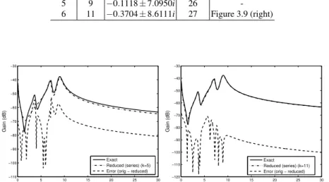
One is especially interested in the peaks and sinks of the Bode magnitude plot, which are caused by the polesandzeros of the transfer functionH. The Modal Truncation[44] is aimed at constructing a reduced order model (3.10) such that peaks and sinks of the reduced order model’s frequency responseGb(ω) =Hb(iω) match with the one of the full dynamical problem (3.4).

Applying Cramer’s rule it is obvious that the transfer function is a rational func-tion:

H(s) = pn−1(s) qn(s) ,

with polynomialspn−1andqnof degreen−1 andnrespectively. The zeros of the

numerator are the zeros of the transfer function and the zeros of the denominator are its poles.

The generalized eigenvalues of the matrix pencil_{E,A_}, or the eigenvalues ofA,

if we assumeE=In×n, are the key to the poles of the transfer function. For a more

detailed discussion we refer to [27]. To illustrate this relation we restrict to the latter case and consider a SISO system without direct feedtrough, i. e.,D=0.

The eigentriples (λi,vi,wi) for i=1, . . . ,n of Aconsist of the ith eigenvalue

λi∈Cand theith right and left eigenvaluevi,wi∈Cn, respectively, that satisfy

Avi=λiv and wHi A=λiwH.

From assuming thatAis diagonalizable it can be derived that LH_AR=Λ,

whereΛ= (λ1, . . . ,λn),R= (v1, . . . ,vn)andL= (w1, . . . ,wn)∈Cn×n, where the

left and right eigenvectors are scaled such thatLH_R=In

×n.

We apply a change of coordinatesx=Rexand multiply the input to state mapping (3.4a) withLH_{which is a projection on the space spanned by the columns ofRalong}

the space spanned by the columns of L. This transforms the input-output system (3.4) to

d

dtex=Λex+LHbu,

y=cHRex.

The transformed system is equivalent to the original system (3.4), the (scalar) trans-fer function can be represented as

H(s) = n

∑

This form of displaying the transfer function is known asPole-Residue Representa-tion, where the quantitiesri∈Care calledresiduesand where we can see that the

eigenvalues of the matrixAare the poles ofH(s).

The idea of modal truncation is to replace the full order problem with a reduced order model of say orderr<nwhose transfer function has a pole-residue

represen-tation that is a truncation of the corresponding full model’s represenrepresen-tation (3.25), i. e. b H(s) = r

∑

whereriandλi fori=1, . . . ,rare the same as in (3.25). The corresponding

state-space representation (3.10) evolves from carrying out the matrix projections defined in (3.11) whereV,W_∈Cn×r comprisesrright and left eigenvectorsv1, . . . ,vrand

w1, . . . ,wr, respectively. As no new poles arise by constructing the reduced order

model in this way, the stability property is inherited from the full order problem. Immediately the question arises, which pairs(λi,ri)of poles and residues and

how many should be taken into account.

Rommes [44] and Martins et al. [30] sort these pairs according to decreasing

dominanceof the pole. Their measure for dominance of a pole is the magnitude of the relation

|ri|

|re(λi)|.

Hence, modal truncation takes into account the firstr poles/residues according to this ordering scheme. The answer to the second part of the question, i. e., how many poles/residues to keep, arises from the error bound [19]

kH−HbkH∞ ≤ n

∑

and hence from the deviation one is willing to tolerate.

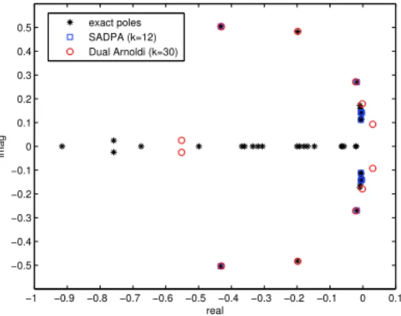
The computation of the error bound (3.27) necessitates a full eigenvalue decom-position. This is only feasible for moderate ordersn≤2000. For large scale systems methods using only a partial eigenvalue decomposition can be applied. Here the

Subspace Accelerated Dominant Pole Algorithm (SADPA), introduced by Rommes and Martins [45] produces a series of dominant poles. The main principle of SADPA is to search for the zeros of 1

H(s) using a Newton-iteration. As the Newton-iteration can only find one zero sufficiently close to a starting value at a time, the iteration procedure has to be applied several times. In order to find less dominant poles at each time, the system the dominant pole algorithm is applied to is adjusted each

time one dominant pole has been found. This adjustment is referred to assubspace acceleration.

Again, for further details we refer to the papers cited above.

3.1.6 Other approaches

We shortly address some other approaches. In [25,39,40], port-Hamiltonian sys-tems are considered to guarantee structure preserving reduced models. In [8,10,11], vector fitting techniques are used to obtain passivity preserving reduced models. In [24, 31, 46], one matches additional moments of Laurent expansions involving terms with 1/s. These are applied to obtain passive reduced models for RLC cir-cuits.

3.1.7 Examples

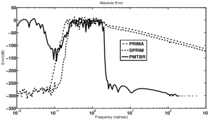
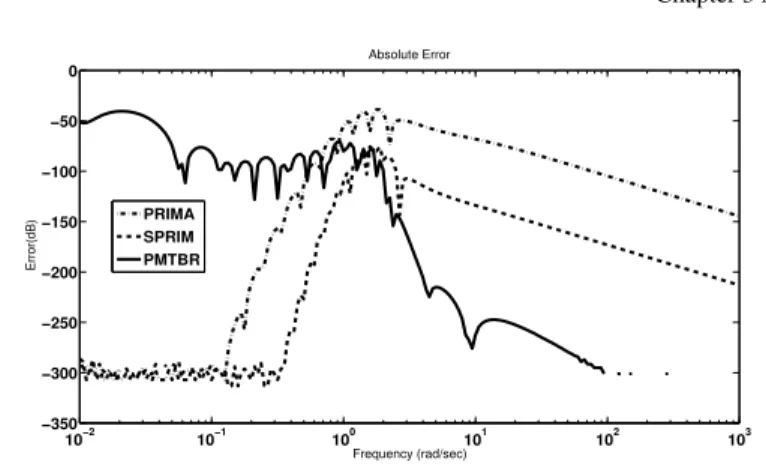
In this part we will introduce linear circuits and reduce them with techniques which have already been discussed. We give results for the methods PRIMA [35], SPRIM [13–17], and PMTBR [36].

In simulation a Bode magnitude plot of the transfer function shows the magnitude of H(iω), in decibel, for a number of frequenciesω in the frequency domain of interest. If the transfer function of the original system can be evaluated at enough pointss=iωto produce an accurate Bode plot, the original frequency response can be compared with the frequency response of the reduced model. In our examples,H is a scalar.

3.1.7.1 Example1

We choose an RLC ladder network [33] shown in Figure 3.1. We set all the capacitances and inductances to the same value 1 while R1= 1₂ andR2=1₅, see

[32, 52]. We arrange 201 nodes which gives us the order 401 for the mathematical model of the circuit.

If we write the standard MNA formulation the linear dynamical system is de-rived. The system matrices are as follows (forK=3, for example):

E=I, A=       −2 0 0 −1 0 0 0 0 −1 1 0 0 ₋5 0 1 1 1 0 0 0 0 ₋1 ₋1 0 0      , B=       0 0 5 0 0      , C=0 0−5 0 0, D=5. (3.28)

Fig. 3.1 RLC Circuit of ordern=2K−1, example 1.

In the state variable x,xk is the voltage across capacitanceCk (k=1, . . . ,K), or

the current through inductorLk−K (k=K+1, . . . ,2K−1). In general the number

of nodesK is odd. The voltageu and the currentyare input and output, respec-tively. Note that when the number of nodes isK the order of the system becomes

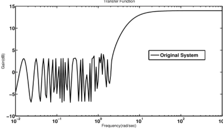
n=2K−1. In this test case we have an ODE instead of a DAE asE=I, see (3.28). The original transfer function is shown in Figure 3.2. The plot already illustrates how difficult it is to reduce this transfer function as many oscillations appear.

10−2 10−1 100 101 102 103 −10 −5 0 5 10 15 Frequency(rad/sec) Gain(dB) Transfer Function Original System

Fig. 3.2 Original transfer function for the first example of Fig. 3.1, ordern=401. The frequency domain parameterωvaries between 10−2_{to 10}3_.

3.1.7.2 Example2

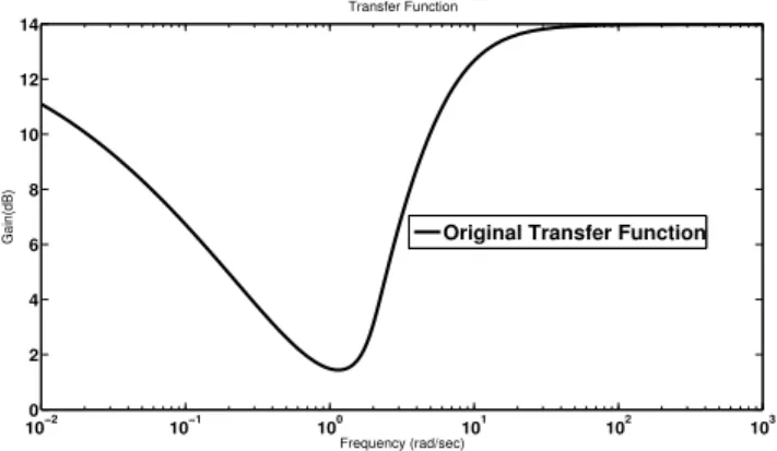
Next, we use another RLC ladder network, given in Figure 3.3 [33, 47], for the second example. The major difference to the previous example is that we introduced a resistor (all of equal value) in parallel to the capacitors at each node connected to