Adaptive blind source separation based on intensity vector statistics.

(1)

Intensity Vector Statistics

A. RIAZ

Submitted for the Degree of Doctor of Philosophy

from the University of Surrey

Centre for Vision, Speech and Signal Processing Faculty of Engineering and Physical Sciences

University of Surrey

Guildford, Surrey GU2 7XH, U.K.

December 2015

(2)

(3)

Human brain has the ability to focus on desired acoustic source when several sources are active. In the domain of digital electronics this problem is termed as the cock-tail party problem. Over the past few decades many algorithms have been proposed which attempt to solve this problem; they are generally termed as acoustic source sep-aration algorithms. The proposed algorithms achieve sepsep-aration of individual source components from observed acoustic mixtures. The source separation system may be capable of estimating the number of sources, their physical locations, the room impulse response and/or any target source signal information. A system that approximates this information is termed as blind. Source separation systems which require any such information beforehand are termed as semi-blind.

Most of the proposed source separation algorithms deal with acoustic sources that are stationary in space. A more challenging task is to approximate unmixing filters while the sources are constantly moving. To maintain output performance in such a scenario, the source separation system has to swiftly and accurately detect the time variant mix-ing parameters, and update unmixmix-ing filters accordmix-ingly. The area of movmix-ing sources has still not been heavily investigated by researchers.

The aim of this thesis is to further the field of acoustic source separation. Investigation of intensity vector direction (IVD) based source separation algorithm was carried out to analyse and improve the system, both in terms of applicability and output sound quality. The algorithm under investigation provides a robust and nearly closed-form solution to the source separation problem with a low processing time. However, the al-gorithm initially required unmixing filter coefficients as input for dealing with practical acoustic scenarios. Analysis performed with microphone array response, microphone array geometry and the room response yielded three different modifications to the baseline system, improving system applicability and output sound quality.

The IVD based system was investigated to deal with more challenging acoustic scenar-ios, such as time variant number of sources. Likewise, the IVD statistics were analysed to propose solutions for moving sources scenario. The system exhibited potential to swiftly, accurately and reliably detect changes in the time varying mixing parameters. As a result of these investigations, a novel system pipeline is proposed, capable of detecting, tracking and separating moving sources in a blind manner.

The proposed algorithms were evaluated for processing time and separation mance. Optimisation of output sound quality was carried out through objective perfor-mance measures, while speaker tracking was evaluated subjectively. Finally, a demon-stration was developed in Matlab based on the proposed algorithms to facilitate user interaction with the surrounding acoustic environment.

Key words: convolutive mixtures, moving blind source separation, Intensity Vector Direction statistics, low processing time, coincident array processing.

(4)

Email: [email protected]

(5)

It gives me great pleasure to acknowledge Prof. Ahmet Kondoz, who gave me the opportunity to pursue a doctorate degree. His enthusiasm and knowledge had a lasting effect and without his guidance, patience and persistent help this thesis would not have been possible. I would like to specially thank Prof. Mark Plumbley for his guidance in improving the presentation of my work. I would like to thank my co-supervisor Dr. Xiyu Shi for always encouraging me throughout these years, and giving me helpful reviews. Last but not the least I would like to thank my parents, my sister and my beloved wife for the never ending love and support.

(6)

arrival in the surrounding space (range of sensitivity = 0-1). Figure-of-eight (solid line ζ = 0), Sub cardioid (dashed-dotted line ζ = 0.7), Cardioid (dashed lineζ = 0.5) . . . 26 2.4 First order B-format Audio . . . 27 2.5 Tetrahedral placement of microphones to form A-format microphone array 28

3.1 Processing stages of the baseline IVD-based system. Initially, the pres-sure and prespres-sure gradient signals are obtained from the microphone array for intensity measurements. Then, the DFT of the signals is mea-sured. Next, the intensity vector directions (IVD) are calculated in time-frequency domain. Next, the von-Mises spatial filters are applied for the known source locations. Finally, IDFTs of the separated signals are cal-culated to get the time-domain estimate of separated sources. . . 34 3.2 The von-Mises spatial filters used for soft masking the time-frequency

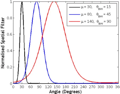
components based on their IVD measurements. The spatial filters are depicted with varying circular means and concentration parameters as mentioned in the legend of the figure. . . 35 3.3 The A-format microphone array with tetrahedral configuration of the

cardioid microphones: Labelled as Left-Forward-Up (LFU), Right-Front-Down (RFD), Left-Back-Right-Front-Down (LBD) and Right-Back-Up (RBU) with respect to the centre of the configuration. Collectively these are known as the A-format signals. The distance of the microphones to center of the array is denoted byr. . . 36 3.4 The SDR (dB) results of varying angular interval between the sources

at different beam-widths of the von-Mises spatial filters. The black line is indicating the trend of increasing SDR as the optimum line. . . 42

(10)

List of Figures v

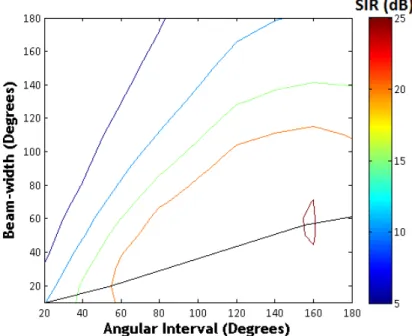
3.5 The SIR (dB) results of varying angular interval between the sources at different beam-widths of the von-Mises spatial filters. The black line is indicating the trend of increasing SIR as the optimum line. . . 42 3.6 Average objective evaluation of two source separation by varying spatial

filter beam-width for baseline IVD system. The overall SDR performance is seen to increase with the increase in spatial filter beam-width (Fig. 3.6a). With a greater spatial filter beam-width, more source components spread around the desired source location are captured. However, as depicted in Fig. 3.6b, consequently more components of the interfering sources are captured as well. Due to this a trade-off exists between signal to interference ratio and signal to distortion ratio. A suitable beam-width applicable to all angular intervals is chosen such that SIR does not fall below a desired threshold (approx. 20 dB). . . 43 3.7 Simulation results of location-based space-frequency IVD measurements

with different microphone array sizes. The limit frequency, highlighted using red vertical line, can be seen to get lower as the array size increases. 46 3.8 Different microphone behaviour depicted for sound originating from

dif-ferent locations to visualise the effect of increased non-coincidence based on source locations. . . 47 3.9 Different directivity patterns of the microphone facing towards 45 degree.

The sensitivity of the microphone array shown to vary from 0 to 1 for different circular directions of arrival. . . 48 3.10 The recording set-up with distances to floor and the ceiling depicted.

The first reflection was found to be approximately 3ms after the arrival time of the direct sound component. With the speed of sound to be 340m s it comes out to be around 1m of distance from the closest reflective surface, which was the ceiling. . . 49 3.11 Method to obtain location-based correction coefficients . . . 50 3.12 Space-frequency microphone response for 70 degrees and 110 degrees.

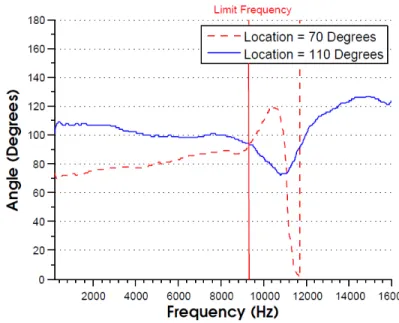
The deteriorating space-frequency response is shown in this figure. It is represented by the deviation of IVD measurements from the physical location of the sources. After a certain limit frequency (approx. 9200 Hz for the array used) the IVD measurements of both the locations can be seen to overlap in space. As this happens the source content originating from these locations is no longer spatially independent. The response of the array at 70 degrees can be seen to phase wrap around after the limit frequency due to aliasing. . . 52

(11)

3.13 The figure depicts IVD measurements of the microphone array through-out the space. It is the complete space-frequency response, with each line representing the IVD measurements from a location in space. Again the space-frequency response is seen to deteriorate significantly after the limit frequency (approx. 9200 Hz). Four distinguished groups can be identified as the four quadrants, with space-frequency response converg-ing at 0 degrees, 90 degrees, 180 degrees and 270 degrees. After the limit frequency is reached (shown as the point of convergence of IVDs) the spatial independence of different locations is compromised due to aliasing at high frequencies. . . 53 3.14 Space-frequency response of ITU-R BS1116 standard listening room with

T60 of 0.32s at 70 degree and 110 degree locations. The room response

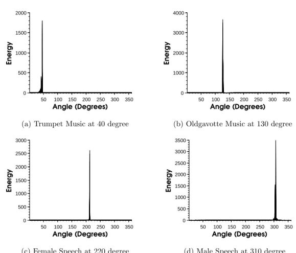
is shown to result in spread of IVD measurements around the physical location of the sources. . . 54 3.15 Energy distribution in space of four sources using the microphone array

response only. The energy distribution is observed to be very compact in space. This figure exhibits the potential of IVD-based system with the microphone array responses low pass filtered at 8000Hz for single sources located at 40, 130, 220 and 310 degrees. . . 55 3.16 Energy distribution of four sources in ITU-R BS1116 standard listening

room withT60 of 0.32s. The energy distributions of the sources in space

are observed to spread around the physical locations of the sources (40, 130, 220 and 310 degrees) as a result of the effect of room response. The energy distributions without the room response have been depicted in Fig. 3.15. . . 56 3.17 Mean and Standard Deviation of IVD measurements with different

re-verberation times - 300Hz to 8000Hz . . . 57 3.18 Energy distribution of four simultaneously active sources at 40, 130, 220

and 310 degrees, considering only the microphone array responses, has been shown to depict the comparison with energy distributions of single sources active alone (Fig. 3.15). The effect of overlapping time-frequency content among sources results in the spread of energy distributions in space as compared to compact energy distribution of sources active alone, as shown in Fig. 3.15. . . 59 3.19 Block diagram of the proposed IVD-based microphone array correction

algorithm. The IVD measurements are corrected using the look-up table and source locations before applying the spatial filters. . . 60 3.20 Corrected space-frequency response of the microphone array shown in

intervals of 10 degrees. The response is observed to improve below the limit frequency as compared to original IVD measurements depicted in Fig. 3.13. See Table 3.2, Table 3.3, Table 3.4 and Table 3.5 for the statistics of corrected IVD measurements in comparison with the original measurements. . . 61

(12)

List of Figures vii

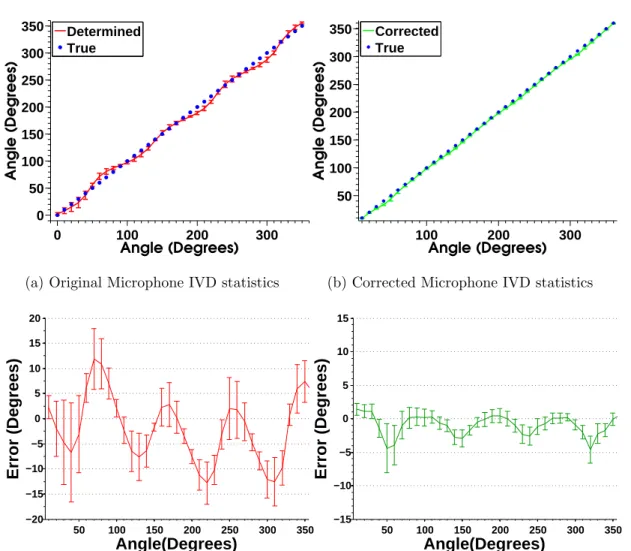
3.21 Mean and Standard Deviation of original (red) and corrected (green) IVD measurements - 300Hz to 8000Hz. See text for discussion. . . 62 3.22 Original and Corrected Mean and Standard Deviation of IVD with

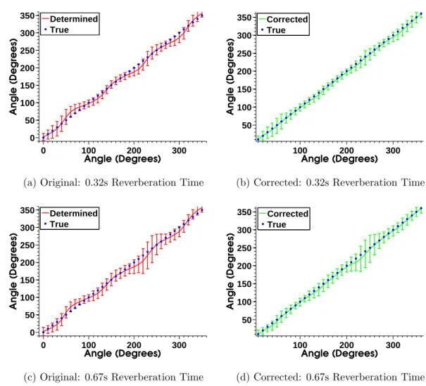
dif-ferent reverberation times - 300Hz to 8000Hz . . . 64 3.23 Block diagram of the proposed system to weight the optimum A-format

microphones using source locations. . . 65 3.24 A-format microphone top view. The closest cardioid microphones are

identified for each source location (highlighted in green). Based on the angular interval, weighting of cardioid microphones is proposed to atten-uate unwanted interference and overlapping time-frequency components impinging at the microphone array from opposite direction to that of the desired source. . . 66 3.25 Block diagram of the proposed system. The Energy and IVD

measure-ments are selected based on their closeness to desired source location using regions of interest. Once the local statistics of the source are lo-cally isolated, spatial filters parameters are set accordingly. . . 68 3.26 Regions of interest for four source locations. The region of interest is

an ideal circular binary filter to locally isolate the IVD measurements of desired sources. . . 69 3.27 Objective evaluation: Adaptation rate of spatial filter parameters . . . . 73 3.28 Block diagram of the proposed IVD-based source separation system

(con-tributions highlighted in green). Initially, the pressure and pressure gra-dient signals are obtained from the microphone array. Then, the DFT of the signals are calculated. Next, the intensity vector directions are cal-culated and consequently the IVD measurements are corrected using the microphone array look-up table. Next, energy weighted mean and stan-dard deviation are used to adapt spatial filter parameters in regions of interest that locally isolate IVD measurements of each source. Based on known source locations, the cardioid weight matrix is determined. For the desired sources, adapted von-Mises spatial filters are used to per-form separation using appropriately weighed microphone signals based on cardioid weight matrix. Finally, the IDFTs of the separated signals are calculated to get time-domain estimates of the sources. . . 75 3.29 Computational time of different processing steps in the proposed system

pipeline . . . 77 3.30 SDR comparison baseline IVD system performance (red) with (a)

Micro-phone array correction (b) Adaptive spatial filters (c) Cardioid weight matrix (d) Combining all modifications, for two source scenario. . . 78 3.31 SIR Comparison of baseline IVD system performance (red) with (a)

Mi-crophone array correction (b) Adaptive spatial filters (c) Cardioid weight matrix (d) Combining all modifications, for two source scenario. . . 80

(13)

3.32 Comparison of baseline IVD system performance (red) with all modifi-cations combined (blue), for two source scenario, RT = 0.67s . . . 81 3.33 Different four sources scenarios considered for experiments - Minimum

angle between any two speakers varying from 30 degree to 90 degree in 20 degree intervals to check systems performance for varying angular intervals. . . 82 3.34 SDR Comparison of baseline IVD system performance (red) with (a)

Microphone array correction (b) Adaptive spatial filters (c) Cardioid weight matrix (d) Combining all modifications, for four source scenario. 83 3.35 SIR Comparison of empirically best selected baseline performance (red)

(a) Microphone array correction (b) Adaptive spatial filters (c) Cardioid weight matrix (d) Combining all modifications, for four source scenario. 84 3.36 Comparison of baseline IVD system performance (red) with all

modifi-cations combined (blue), for four source scenario, RT = 0.67s . . . 85

4.1 First order IIR filter structure . . . 92 4.2 IVD Distribution in space (a) Without von-Mises modelling (b)

Apply-ing first order IIR Filter to smooth out noise in the time domain (c) Modelling the IVD with von-Mises distribution funtion to smooth out noise in space (d) Applying von-Mises model along with first order IIR filter to achieve denoised IVD distribution in both time and space. . . . 93 4.3 Effect of distance of the speaker to microphone array on IVD distribution

in space. (a) Ground truth (b) IVD distribution in space. Speaker 1 is moving forwards and backwards w.r.t to the microphone array while Speaker 2 is stationary in space. The closer the speaker gets, the greater its captured energy and its direct to reverberant ratio. As a result it has better IVD distribution representation in space (prominent with a high peak). The distribution of a physically stationary Speaker 2 is also shown to get affected due to the change in distance of Speaker 1. . . 94 4.4 IVD distribution of two moving speakers at the same distance to the

mi-crohone array. (a) Ground truth (b) IVD distribution in space. Speaker 1 is moving between 75 degrees and 125 degrees, while Speaker 2 is moving between 175 and 225 degrees. . . 96 4.5 Processing stages of the baseline IVD-based system (see Section 3.2).

Initially, the pressure and pressure gradient signals are obtained from the microphone array. Then, the DFT of the signals is measured. Next, the intensity vector directions are calculated in time-frequency domain. Next, von-Mises spatial filters are applied for the known speaker loca-tions. Finally, IDFTs of the separated signals are calculated to get the time-domain estimates of the target speakers. . . 97

(14)

List of Figures ix

4.6 The utilisation of time-frequency units up to 4000Hz to up to 22050Hz for IVD distribution representation. Speaker 2, which is distant (approx. 3 meters) to the microphone array portrays less prominent IVD distri-bution with increase in the frequency range until it completely becomes part of the IVD distribution floor. Also with the increase in frequency range, IVD distribution of Speaker 1 can be seen to spread in space. . . 99 4.7 Log IVD distribution with IIR filtering corresponding to different

aver-aging times (a) 46.4 ms (b) 185.8 ms (c) 278.6 ms (d) 371.5 ms. As the effective averaging time increases, the IVD distribution becomes more regular and denoised to reveal reliable estimates of the speakers; how-ever, averaging over a much longer period of time leads to poor speaker estimates, because longer averaging times may result in multiple peaks for the same speaker due to a slow update rate of the IVD distribution (4.8). . . 101 4.8 Peak Detection & Location Expectation with IIR filtering corresponding

to different averaging times (a) 46.4 ms (b) 185.8 ms (c) 278.6 ms (d) 371.5 ms. The red cross indicates the time delay caused in peak detection due to longer averaging times. See text for discussion. . . 102 4.9 Average IVD distribution measurements over 2.5s of recorded speech

activity: (a) Two Speakers (b) Four Speakers. The average IVD distri-bution peaks are higher and more prominent for less speakers. With a greater number of speakers the IVD noise floor gets high due to added reverberations and increase in overlapping time-frequency content of speakers, resulting in a poor IVD distribution representation. Due to poor IVD representation over short time durations, added speakers pose a challenge to the moving blind source separation system. . . 104 4.10 (a)-(c) IVD distribution for different number of speakers (d)-(f) Peak

Detection results - high static threshold = 1.5 (g)-(i) Peak Detection results - adaptive to number of speakers detected (j)-(l) Peak Detection results - low static threshold = 0.5. (Red ellipses show errors. See Section 4.4.2.1 for discussion.) . . . 107 4.11 Peak detection and location expectation using different increment values

in the location expectation usingp. The false peaks are circled in red for clarity in analysis. The amount of false detections can be observed to reduce as the delay in speaker detection increases from an instantaneous value to 0.3s. . . 110 4.12 Peak detection and location expectation using different increment values

in location expectation usingp. Red arrows represent delay in time while detecting a new speaker. See the text for discussion. . . 111 4.13 Peak detection and location expectation using different decrement values

in the location expectation by varyingq. Green arrows show the waiting time before declaring a speaker as absent. See the text for discussion. . 112

(15)

4.14 Block Diagram of Proposed Moving BSS System (contributions high-lighted in blue). Initially, the pressure and pressure gradient signals are obtained from the array. Then, the DFT of the signals are calculated. Next, the intensity vector directions are calculated and consequently IIR filtered IVD distribution in space is measured using von-Mises mod-elling of the IVD measurements. Next, peak detection is done to locate potential speakers in the surrounding space. Location expectations are assigned to the identified peaks for reliable speaker detection and to cater for pauses in between speech activity. For the detected speakers time-variant von-Mises spatial filters are designed and applied. Finally, IDFT of the separated signals are calculated to get the time-domain estimates of target speakers. . . 113 4.15 Computational time of proposed BMSS algorithms with respect to

num-ber of speakers. See the text for discussion. . . 115 4.16 Experimental Setup: (a) Stationary source locations (b) Regions of

speaker movement. A maximum 60 degree interval of speaker move-ment is assigned for each region in the designed set-up. It is to be noted that the proposed system can perform speaker detection, tracking and separation even if the speaker moves out of the allocated region, as long as it does not co-locate with other active speakers. . . 116 4.17 Examples of two moving speakers - Tracking and detection performed

by the proposed BMSS system. In (a) and (c) the location expectation of speakers is depicted to show tracking. Separate ‘tracks’ of speaker movement can be observed in space. Near the time frames in the middle (800 - 1200), the speakers take a long pause and start speaking again while carrying out movements. In (b) and (d) the true speaker activity is compared with the activity determined by the proposed BMSS system. 119 4.18 Two speaker mixtures: PEASS Toolbox results showing comparison

between baseline IVD implementation and BMSS system with moving speakers and stationary speakers. See text for discussion. . . 122 4.19 Two speaker mixtures: BSS Eval Toolbox results showing comparison

between baseline IVD implementation and BMSS system with moving speakers and stationary speakers. See text for discussion. . . 123 4.20 Examples of four moving speakers - Tracking and detection performed by

the proposed BMSS system. In (a) the location expectation of speakers is depicted to show tracking. In (a) separate detected ‘tracks’ of the four speakers in space can be observed. Near the time frames in the middle (800 - 1200), the speakers take a long pause and start speaking again while carrying out movements. In (b) the true speaker activities are compared with those determined by the proposed BMSS system. . . 124 4.21 Four speaker mixtures: PEASS Toolbox results showing comparison

between baseline IVD implementation and BMSS system with moving speakers and stationary speakers. See text for discussion. . . 126

(16)

List of Figures xi

4.22 Four speaker mixtures: BSS Eval Toolbox results showing comparison between baseline IVD implementation and BMSS system with moving

speakers and stationary speakers. See text for discussion. . . 127

A.1 Graphical user interface of BSS application . . . 137

A.2 Device connected panel . . . 138

A.3 Control Panel in GUI . . . 138

A.4 Rate of spatial filter adaptation panel . . . 139

A.5 Figures panel . . . 139

(17)

Symbols ¯

c(t) Threshold for peak detection ¯

K Average approximated IVD distribution floor ¯

rn Resultant vector for source n

˘

D Diagonal scaling matrix

˘

I Permutation matrix

δi(f, t) Relative delay between microphones n Location expectation of speaker n

ˆ

d Smallest distance considering Nyquist theorem ˆ

F A-format to B-format conversion matrix ˆ

f(θ) Microphone response at angle θ

ˆ

I Identity matrix

ˆ

k Window sample index

ˆ

M Window size in samples

ˆ

m Mask used in time-frequency filtering ˆ

P Power

ˆ

sn Separated source n

ˆ

W Additive noise data

ˆ

w Window function

Λ Cross-section area

λmin Smallest wavelength considering Nyquist theorem µ Mean circular direction of von-Mises distribution

(18)

List of Figures xiii

ν Volume

Øn Region of Interest for source n

ω Angular Frequency

φ Phase

ρ Density

σ Concentration of von-Mises distribution around mean location

θ Circular variable for von-Mises distribution

θd Angular interval of source location from cardioid microphone

orien-tations

θBW Beam-width value

θLBD LBD cardioid microphone orientation angle θLF U LFU cardioid microphone orientation angle θRBU RBU cardioid microphone orientation angle θRF D RFD cardioid microphone orientation angle

ζ Microphone weighting to determine directional response

A Extent of displacement

a Acceleration

Af A-format data matrix

ai(f, t) Relative amplitude between microphones

B Unmixing matrix

c Speed of sound

Cn(ω, t) Corrected time-frequency IVD for source n

D Energy Density

d Array vector

E Energy

Ek Kinetic Energy

Ep Potential Energy

f(θ;µn, σn) Spatial filter with µdirection andσ beam-width for source n

(19)

f Frequency

Gi Cluster centre representing source i H Room Transfer Function Data

h Elastic Constant

I Intensity

Jn Subset of Cn based on region of interest

k Wave number

Ln Index of correction vector for source n

M Number of microphones

m mass

N Number of sources

P Pressure

p Increment value in speaker location expectation

p(si) Probability density function of i-th source p(s1, s2, s3...sN) Joint probability density function of sources PBLD A-format Back-Left-Down pressure signal PBRU A-format Back-Right-Up pressure signal PF RD A-format Front-Right-Down pressure signal PLF U A-format Left-Front-Up pressure signal Q Resolution factor of correction

q Decrement value in speaker location expectation

r Radial Distance

r(θ, f) Beam-former response at angle θand angular frequencyω

S Source data

t Time

U Cardioid weight matrix

V Velocity

W Inverse of room transfer function

(20)

List of Figures xv

WB B-format omnidirectional response

X Mixture Data

XB B-format figure-8 response across x-axis

Y Separated source data

YB B-format figure-8 response across y-axis Zn(ω, t) IVD correction vector for source n

Abbreviations

ASIO Audio sound input output

BSS Blind Source Separation

CASA Computational Auditory Scene Analysis

CLT Central Limit Theorem

DF T Discrete Fourier Transform

DOA Direction of Arrival

DU ET Degenerate Unmixing Estimation Technique

ECG Electrocardiogram

EEG Electroencephalography

GP S Global Positioning System

GU I Graphical user interface

ICA Independent Component Analysis

IDF T Inverse discrete Fourier transform

ILD Inter-aural level difference

IT D Inter-aural time difference

IV D Intensity Vector Direction

M L Maximum Likelihood

M M SE Minimum Mean Square Error

OS Operating system

P CA Principle Component Analysis

P DF Probability Density Function

(21)

SI Standard International

SIR Signal to Interference Ratio

ST F T Short Time Fourier Transform

(22)

Chapter 1

Introduction

Audio information is processed during many activities in the daily life of a human. Through perceived acoustic signals, people are able to extract valuable information about their surrounding environment. Even in a reasonably crowded room, a person with healthy hearing is able to identify and focus on a particular acoustic source of interest. Such source of interest may be a musical instrument, a single speaker or multiple speakers having a conversation among a number of interfering sources. The ability of humans to perform such acoustic tasks is referred to as the solution to the cocktail party problem [1].

Intense research has been conducted in the domain of digital signal processing over last few decades to try and mimic the human ability to perform a range of acoustic tasks. These include source detection, source identification, source localisation, source tracking and source separation. A result of such research is the Computational Auditory Scene Analysis (CASA). CASA is the approximation of human auditory system to localise and isolate acoustic sources of interest [2]. Other approaches also exist which try to solve the problem of source separation purely based on mathematics. These approaches try to exploit source signal properties and the environment transfer function.

A significant number of source separation techniques rely on the microphone arrays to perform separation [3][4]. Such arrays comprise of a number of microphones arranged in a single or multidimensional configuration. This thesis deals with a compact coinci-dent microphone array, comprised of four cardioid microphones placed in a tetrahedral

(23)

Source Separation

System

Source 1

Source N

Source 1

Source N

Figure 1.1: Source Separation System

configuration. Mixture signals recorded by the microphone array are processed with source separation algorithm to output individual sources in separate channels.

Blind Source Separation (BSS) refers to the problem of source separation when no prior mixing information is available. This information can be in the form of number of sources, the location of sources, knowledge of Room Impulse Response (RIR) and/or any target source signal information. In more challenging source separation scenarios, added information includes the speed with which sources and/or the microphone array moves, and the time at which a particular source enters and/or leaves the acoustic scene. In a real environment, the source signals are not only directly captured by the microphone array, but the time delayed reflections are also part of the recordings. This further complicates the source separation problem. The information of mixing is contained in the RIR [5]. Most commonly, the RIR contains direct sound from sources and, their reflections and reverberations as a result of source interaction with the surrounding environment.

Some of the source separation techniques utilise spatial diversity to perform separation of sources [6]. Having the knowledge of target source location or interfering sources, a desired spatial response can be constructed to extract the source of interest. Adaptive methods have also been proposed which modify the spatial response of the microphone array according to the perceived source signals [3][4]. A different approach based on

(24)

1.1. Applications 3

the statistical properties of microphone signals rather than spatial diversity also exists [7][8]. These different types of algorithms are still widely under investigation. The choice of algorithm is purely based on the application requirement and implementation environment. The requirements include, but are not limited to, real-time or off-line processing [9][10], compactness of the microphone array [11] and the number of sources to be separated [12][13]. For example, in a small electronic device such as a hearing aid, the integration of a compact microphone array is desired.

Blind source separation is a multifaceted problem, as such, the issues that need to be addressed include degraded performance with increase in reverberation time [14], sources located close to one another [11], coping with greater number of sources [15], localisation of sources [16], source activity detection and most importantly the sce-nario of moving sources [17][18]. Over the past decade considerable research has been carried out for physically stationary sources [19][13][20][21][22]; comparatively, the par-ticular problem of separation of moving sources has not been extensively investigated [23][18][24]. It is unrealistic to consider a source as stationary in daily life scenarios, for example, a professor may move around while delivering a lecture. The movement of sources poses a challenging problem to the researchers. The aim is to constantly detect changes in mixing conditions and update unmixing system parameters accordingly with a low latency, to maintain output sound quality of the source of interest.

1.1 Applications

Blind source separation is essentially a complex mathematical problem. The solution of this problem has direct impact on many applications of signal processing. It can be used in video conferencing, to obtain desired speakers voice and possibly direct the camera towards the speaker of interest using localisation cues.

Speech and speaker recognition systems need interference free voice to perform effective recognition. In a car while giving voice commands, the cell phone or a Global Position-ing System (GPS) does not necessarily capture only drivers voice. It is possible that interfering sources are active, or the noise of car engine or a nearby air-conditioning system may corrupt the drivers voice beyond recognition. As such, in hands-free human

(25)

computer interaction, it is essential to separate the speaker of interest from unwanted interfering sources and carry out voice commands. Similar concept can be applied to suppress interfering sources while carrying out communication over the internet, for example while communicating over Google Hangout or Microsoft Skype.

The ability of humans to listen and process sound present in the surrounding environ-ment is extremely important in day to day life. Some human beings lose the ability to hear as they get older. Not only low energy sounds become hard to recognise, frequency dependent loss may also develop. When multiple speakers are active at the same time, it becomes more difficult for humans with less ability to hear out the speaker of interest. High quality hearing aids with blind source separation algorithm are used to reduce their listening effort and improve speech intelligibility.

Acoustic surveillance is another important application of blind source separation. It can be used by security agencies for spying and intelligence related purposes. The separated output and source localisation cues can be used in forensic analysis as well. Also, in underwater acoustics blind source separation has the ability to detect, separate and facilitate understanding of underwater acoustic events. These include tracking ship movements, and detecting gas or oil leakages.

1.2 Scope and Objective

Aiming to achieve a deterministic and low complexity source separation system, the Intensity Vector Direction (IVD) based algorithm was developed by Gunel et al. [11]. The purpose of this thesis is to further the field of source separation by investigating and improving the IVD-based source separation system for practical acoustic scenarios. As such, this thesis deals with analysis and improvement in applicability and output sound quality of the IVD-based system, while dealing with stationary and moving sources scenarios.

The scope and objectives of this thesis include:

1. To fully understand and investigate the existing IVD-based source separation system.

(26)

1.3. Thesis Outline 5

2. To propose new algorithms for improving output sound quality and applicabil-ity of existing IVD-based source separation system, wherever shortcomings are identified.

3. To investigate existing source separation system to perform blind source separa-tion in practical acoustic scenarios, including but not limited to moving sources. 4. To propose new algorithms to develop IVD-based source separation system in order to perform separation in practical acoustic scenarios, including but not limited to moving sources.

1.3 Thesis Outline

Over the past few decades several types of source separation techniques have been proposed which deal with physically stationary sources, while only a few have been proposed to deal with moving sources. Related techniques in the field of source separa-tion are discussed in Chapter 2. Source separasepara-tion techniques can be widely categorized into three distinct groups. These are the statistical, beam-forming and time-frequency sparsity-based source separation techniques, presented in Section 2.1.2, Section 2.1.3 and Section 2.1.4 respectively. The background of sparsity-based IVD technique is highlighted in Section 2.2 to facilitate the understanding of its foundations.

Analysis and improvement of IVD-based source separation system for stationary sources scenario is presented in Chapter 3. The baseline IVD-based source separation technique is presented and evaluated in Section 3.2 to support the novelty of contribution chap-ters. The system is investigated with respect to microphone array (Section 3.3.2), surrounding room environment (Section 3.3.3) and impact of multiple sources on the time-frequency IVD measurements (Section 3.3.4). Algorithms are proposed to com-pensate for the non-ideal behaviour of microphone array (Section 3.4), select the most suitable microphones to separate the source of interest with a superior output qual-ity (Section 3.5) and adaptively cater for the room response and interfering sources (Section 3.6).

(27)

Later, the IVD-based source separation system is investigated to perform in practi-cal acoustic scenarios, which include time-variant activity of the sources and moving sources. In Section 4.3, a new analysis with respect to IVD distribution in space is presented for practical acoustic scenarios. The analysis is carried out to recognise and exploit the full potential of existing IVD-based system in order to perform source activ-ity detection and tracking. To develop IVD-based system into a blind source separation system capable of dealing with practical acoustic scenarios, denoised IVD distribution (Section 4.4.1), adaptive peak detection (Section 4.4.2), and location expectation (Sec-tion 4.4.3) algorithms are proposed.

Finally, the IVD-based blind source separation demonstration developed in Matlab 2012b with the proposed algorithms is presented in Appendix A. The graphical user interface (GUI) of the developed application is discussed in Appendix A.2. It facilitates setting up the recording equipment and provides GUI to interact with surrounding acoustic sources in real-time. The detected and tracked sources are displayed as options on GUI to allow the user to choose among several active sources (Appendix A.2.5). As a result the sources can be listened to in any desired combination and real-time plots on the GUI show the IVD statistics as they vary with time (Appendix A.2.4).

1.4 Original Contributions

1. A new analysis of the IVD-based source separation system is presented utilising a real microphone array measurements and room impulse responses.

2. A new measurement-based microphone correction algorithm is proposed in Sec-tion 3.4 to provide better localisaSec-tion cues, and it is evaluated for two different room environments.

3. A new algorithm is proposed to select and weight cardioid microphones based on the desired source locations (Section 3.5). It is proven to give superior output sound quality.

4. An energy weighted algorithm is proposed to adaptively update the spatial filter parameters in a non-exhaustive manner, based on local statistics of the IVD

(28)

1.5. Publications by the Author 7

measurements (Section 3.6).

5. A new analysis to deal with practical acoustic scenarios with respect to IVD distribution in space is presented in Section 4.3.

6. Based on IVD statistics, a new blind moving source separation system pipeline, capable of speaker detection, localisation, tracking and eventually separation, is proposed to deal with practical acoustic scenarios in Section 4.4.

1.5 Publications by the Author

1. A. Riaz, X. Shi, A. Kondoz, “Adaptive Blind Moving Source Separation based on Intensity Vector Statistics”, submitted to IEEE/ACM Transactions on Audio, Speech and Language Processing.

2. A. Riaz, X. Shi, A. Kondoz, “Adaptive Source Separation of Convolutive Mixtures based on Intensity Vector Statistics”, to be submitted, IEEE/ACM Transactions on Audio, Speech and Language Processing.

(29)

Related Work

Acoustic blind source separation is the problem of automated separation of audio sources from observed mixtures. It is commonly known as the cocktail party prob-lem. The cocktail party problem is described as focusing on one active speaker in a room where multiple speakers are simultaneously active. It was first clearly defined by Colin Cherry [25]. For humans it is not difficult to pay attention to one of the speakers; however, for machines the problem is still being widely investigated. Re-search has been carried out over the past few decades to study several aspects related to the cocktail party problem. These include localisation of sound sources, geometry of the microphone array, processing complexity of the algorithm, room impulse response identification, identifying time-variant mixing system parameters for moving sources, approximating time-variant number of sources and estimating any target source signal information. Although this thesis focuses on acoustic BSS, the mathematical implica-tion of these techniques is useful in other areas as well, such as in image processing and medical signal processing [26].

In this chapter, first the related work in the field of source separation is presented. It is followed by the background of IVD-based source separation system and a discussion on the microphone array used for intensity measurement.

(30)

2.1. Related Work 9

2.1 Related Work

The most widely used methods for performing source separation are the statistical methods, such as ICA [7][8]. Second category of methods rely on the microphone array configuration entirely, for example the adaptive beam-forming [3][4]. The remaining methods, like DUET [27], exploit time-frequency sparsity among source signals to per-form separation.

The BSS problem for M microphones and N sources for stationary sources scenario can be generally represented as [28]:

X(t) =HS(t), (2.1)

where N number of source signals are S(t) = [s1(t)s2(t)s3(t)...sN(t)]T. The

trans-fer function coefficients are contained in (M ×N) mixing matrix H, such that hmn

represents coefficient form-th microphone andn-th source. X(t) = [x1(t)x2(t)x3(t)... xM(t)]T contains the resultant mixture components of M microphones. The task is

to extract source signals S(t) from observedX(t) mixtures. The two mixture models which are considered while solving the blind source separation problem are presented first. It is followed by a discussion on blind source separation techniques that are being actively investigated.

2.1.1 Source Mixture Models

The instantaneous and convolutive mixture models define the mixture signals encoun-tered while dealing with source separation problem.

2.1.1.1 Instantaneous Mixture Model

The instantaneous mixture model assumes that the sensors measure only scaled version of the sound sources at every time instantt. For three sources and three microphones scenario, this model is mathematically represented as [29]:

(31)

     x1(t) x2(t) x3(t)      =      h11 h12 h13 h21 h22 h23 h31 h32 h33           s1(t) s2(t) s3(t)      +      ˆ w1(t) ˆ w2(t) ˆ w3(t)      . (2.2)

The sources are assumed to be physically stationary in this representation. s1(t),s2(t)

ands3(t) represent the source signals and ˆwn(t) represents the additive noise. h12

rep-resents the time-invariant transfer function coefficient from sources1to the microphone x2. Likewise, other transfer function coefficients between sources and microphones are

contained within the hmn coefficients matrix. x1(t), x2(t) and x3(t) are the resultant

acquired mixtures. For a general scenario with M microphones and N sources, the representation for instantaneous mixture model can be done as:

X(t) =HS(t) + ˆW(t). (2.3)

The instantaneous mixture model is the simplest form of modelling a mixture of signals. It implies that source signals are only being amplitude modulated, not time delayed or echoed. It represents an ideal surrounding environment where reverberation or multipath propagation is absent. The instantaneous mixture model is most commonly used for research purposes while dealing with acoustic applications. Several other signal processing applications of the instantaneous mixture model also exist [30][26], such as in image processing, to extract independent features of an image in order to denoise and improve overall image quality [26]. It is also applicable in medical signal processing, for example when the underlying components of brain activity have to be identified from given recordings in the form of an electroencephalogram (EEG) [30]. The ideal instantaneous mixture model with respect to acoustic sources and microphones is depicted in Fig. 2.1.

2.1.1.2 Convolutive Mixture Model

In practical acoustic scenarios, source separation algorithms must take convolutive mixing of the acoustic sources into account, as the multipath effects of real reverberant

(32)

2.1. Related Work 11

Figure 2.1: Instantaneous Mixture

environment cannot be ignored [31]. As compared to instantaneous mixture model, the received signals not only contain scaled version of source signals but also their filtered and dispersed versions. In a reverberant room, this phenomenon takes place due to different times of arrival of direct sound, reflected sound and reverberating sound. It makes source separation problem much more challenging to solve, especially when the reverberation time is great. The mathematical representation of three sources and three microphones scenario for a convolutive mixture model is [29]:

x1(t) = [h11(t)⊗s1(t) +h12(t)⊗s2(t) +h13(t)⊗s3(t)] + ˆw1(t) (2.4) x2(t) = [h21(t)⊗s1(t) +h22(t)⊗s2(t) +h23(t)⊗s3(t)] + ˆw2(t) (2.5) x3(t) = [h31(t)⊗s1(t) +h32(t)⊗s2(t) +h33(t)⊗s3(t)] + ˆw3(t). (2.6)

Here ⊗ denotes convolution, sn(t) represents source signals, hmn(t) represents the

transfer function between then-th source and m-th microphone, and xm(t) represents

the obtained mixtures. ˆwm(t) represents the additive noise component. Using matrix

notation it can be written as:

X(t) = [H(t)⊗S(t)] + ˆW(t). (2.7) Convolution in time domain corresponds to multiplication in the frequency domain, therefore equation (2.7) can be rewritten for frequency domain representation as:

X(ω) = [H(ω)S(ω)] + ˆW(ω). (2.8)

(33)

Figure 2.2: Convolutive Mixture

2.1.2 Statistical Methods

Independent Component Analysis (ICA) was first clearly defined in 1994 by P. Comon [8] after initial work done with Jutten and Herrault [32]. It is a statistical technique, used to expose underlying hidden components from sets of observed measurements. ICA can be seen as an advancement of Principal Component Analysis (PCA). In its simplest form it was proposed to solve the instantaneous mixture model; however, for real environments ICA has to deal with convolutive mixtures and it increases in computational cost due to increase in FIR filter length. To overcome this problem, frequency domain implementation of the ICA algorithm is carried out [31]. ICA for instantaneous mixture model forms the basis for dealing with convolutive mixtures. It is essentially parallel execution of a series of instantaneous ICA at each frequency bin. In order for ICA to perform unmixing, some assumptions need to be made [33]. Firstly, the source components are assumed to be statistically independent. Mathematically it implies that the joint Probability Density Function (PDF) is factorizable as [34]:

p(s1, s2, s3...sN) = N Y

i=1

p(si). (2.9)

For example two random variables,sx andsy, are said to be independent if there is no

mutual information among the two, i.e. information ofsxdoes not give any information

ofsy, and vice versa. Although the source signals are independent, the mixture signals, xm, are not. As such, the underlying independent source components are extracted by

(34)

applying ICA on mixture signals. ICA performs source separation by exploiting higher order statistics of the signals. The higher order cumulants of the Gaussian distribution are zero, implying that independent components of each source should ideally have non-Gaussian distributions.

Another assumption made for ICA is that the mixing matrix is invertible. As a result, the number of sources is equal to or less than the number of microphones. For specific scenarios, where the number of microphones and sources may vary,M greater thanN

case is termed as overdetermined, M less than N is termed as underdetermined and

M equal to N is termed as a determined case. The time-frequency content of sources can be exploited to solve the underdetermined case as well [13]; however, it requires additional processing steps.

Considering the noise free version of equation (2.3), the ICA solution exists in having an unmixing matrixW such that:

S(t) =W X(t). (2.10)

The time relation will be dropped in the following representations for simplicity. Coef-ficients of W can be found using prior measurements of the transfer functionH. This however is not a practical solution. ICA instead finds the coefficients ofB such that:

BH = ˘ID,˘ (2.11)

where ˘D is a diagonal scaling matrix and ˘I is an (N×N) permutation matrix. Hence, the separated statistically independent sources can be found as:

Y =BX. (2.12)

Here Y represents the statistically independent components of separated sources, ob-tained from processing the mixture signals,X. There are several techniques for solving the instantaneous ICA problem.

(35)

2.1.2.1 PCA Preprocessing

For performing ICA, the sources are assumed to be independent, and as such, their joint PDF can be represented in the form of equation (2.9). PCA preprocessing can be used to decorrelate the mixturesX prior to performing ICA [8]. Independence implies decorrelation and not the vice versa. PCA preprocessing facilitates ICA by performing decorrelation over the lower order statistics. It results in a transformation of X such that:

Ex´x´T = ˆI, (2.13)

where ´x represents the transformation of X and it is whitened data with resulting correlation matrix ˆI, a unit matrix. This is done only for dealing with the second order statistics of the signals. In order to achieve complete independence, the signals are to be processed for all orders using ICA. Therefore PCA is used as a preprocessing stage for ICA to decorrelate the data, reduce noise, reduce computations and achieve a quicker convergence [35].

2.1.2.2 ICA-based Techniques

ICA has developed as a general concept representing a family of techniques which aim to extract independent source signals. From the central limit theorem (CLT) it is known that the sum of independent signals tend to be more Gaussian than any of the two signals considered alone [36]. Hence independence implies non-Gaussianity, as such, in ICA an unmixing matrix (W) is found such that non-Guassianity of individual source signals is maximised. ICA removes dependence in higher orders (after PCA preprocessing) and hence ICA is often termed as the rotation which makes decorrelated data independent [26]. For achieving independence, higher order statistics such as kurtosis are used. Iterative methods are utilised to either maximise or minimise the considered cost function, such as related to kurtosis [37] or mutual information entropy [8]. All the cost functions relate to non-Gaussianity to an extent. As such, ICA has been formulated with several implementation approaches:

(36)

1. Maximum Likelihood (ML) [38][39][40]

2. Maximisation of information transfer [41][42][43] 3. Negentropy [44]

4. Higher order moments and cumulants [8][45] 5. Non-linear PCA [46][47][48]

These approaches are based on cost functions that try to exploit non-Gauassanity of source signals. The reasons for using different cost functions is related to computational cost or sensitivity to outliers. There are several gradient descent methods available for using these cost functions in order to derive unmixing matrix,W. These include Newton method of descent [35], steepest gradient descent and stochastic gradient descent [49]. The natural gradient descent method is one of the most commonly used methods for performing ICA [50].

ICA algorithms for instantaneous mixture model can be applied at each frequency bin in frequency domain to deal with convolutive mixtures. Commonly, a Short Time Fourier Transform (STFT) is used for framing the time data and transforming each time frame into the frequency domain. As such, the representation of signals is carried out as

x(f, t), h(f, t) and s(f, t) exhibiting a dependence on both the time and frequency [51].

2.1.2.3 Limitations of ICA

In ICA there are ambiguities with regards to order and scaling of the separated source signal components. It is due to the permutation matrix, as given in equation (2.11). The problem extends to each frequency bin while dealing with convolutive mixtures. The permutation ambiguity is described as the mixing up of estimated independent sound source components due to lack of proper alignment [13]. The permutation ambiguity is faced because bothS and H (equation 2.1) are unknown, so the order of components can get exchanged even after the independent source components have been determined [52].

(37)

Although many post processing algorithms have been proposed to designate the sep-arated independent components to their corresponding sources, permutation problem has no closed form solution [53]. The proposed solutions either utilise time-frequency source models, exploit room impulse response or use the array geometry information [31][54][55][56][57][52]. The post processing required to solve permutation problem adds to the computational cost, and as no closed form solution exists, it is still being widely investigated [58][53].

Another ambiguity faced by ICA is the scaling ambiguity [52]. Although it is not as severe as the permutation ambiguity, it occurs when the energy of independent components does not relate to the energy of source signals. Since both S and H are unknown, any scaling of source signalSi could be made ineffective by scaling down the

corresponding columnHi inH: X=X i 1 αHi (αSi). (2.14)

This problem is commonly resolved by normalising the unmixing matrixW [59]. Another issue with ICA is the assumption of linearly stationary mixing conditions, i.e. the mixing matrix is assumed to be constant, independent of the time-variant source signals [60]. This assumption degrades the effectiveness of ICA in real life scenarios, for example, during electrocardiogram (ECG) the mixing conditions change over time when the person inhales or exhales [61]. Also, in acoustic applications, moving sources lead to changes in the mixing conditions [62], which are inherently assumed to be stationary by ICA. As such, this assumption creates problems while using ICA in more practical scenarios.

At the final stage, the approximated unmixing matrixW is used to perform separation in the time-frequency domain using STFT as:

y(f, l) =W (f, l)x(f, l), (2.15)

where y(f, l) = [y1(f, l), y2(f, l)...yN(f, l)]T contains the source estimates, W(f, l)

is time-frequency representation of unmixing matrix andx(f, l) = [x1(f, l), x2(f, l)... xM(f, l)]T represents the obtained sound mixtures.

(38)

2.1.3 Beam-forming Methods

Despite using microphone array information for solving the permutation problem, ICA methods fundamentally rely on statistical independence of source signals [8]. A separate category of algorithms exists which performs source separation based on the knowledge of microphone array geometry [3][4]. Commonly termed as beam-forming [63], these methods can be used to spatially separate out data from the desired locations. The sensors of the array are located at different points and as a result are able to sample the incoming sound wave in space. The acquired data is then processed to attenuate interfering signals and extract desired source signal. Some of these techniques focus on finding the Direction Of Arrival (DOA) to perform spatial filtering.

The beam-forming methods work on the same principle as that of a simple digital filter. In a digital filter the signals are passed or stopped depending on their frequency content. Spatial diversity can be exploited in a similar manner of passing or stopping the source signals depending on the direction of arrival. It is commonly achieved by delaying parts of the input signal and multiplying by weights. In a beam-former, simple tap delays correspond to the weights that result in spatial filtering. Despite having overlapping frequency content, the signals can be recovered due to their different locations in the surrounding environment [63].

Using beam-forming technique for the desired source, a weight vector wis used in the frequency domain to perform source separation [63]:

y(f) =w(f)Hx(f), (2.16)

where x(f) is the mixture and y(f) is the separated source. Here H denotes the Hermitian operator. Due to geometry of the microphone array, there is a physical delay in time of arrival of sound at each microphone, given by [63]:

d(θ, f) =

h

1, e−j2πf τ1_{, e}−j2πf τ2_{, ... , e}−j2πf τM−1iT_. _(2.17)

The physical delay is a function of the source direction θ and frequency f. It is to be noted that there is no delay at the first microphone as it is taken as the reference.

(39)

Considering the frequency dependent filter coefficientsw(f), the beam-former response with respect to source directionθ is given as [63]:

r(θ, f) =w(f)Hd(θ, f). (2.18)

The weights of the beam-former are determined such that the desired source adds constructively at the output [64]. Source signals from other than the desired source location are filtered due to different time lag at each microphone.

It is a well known fact that the sampling rate must be at least twice the highest frequency component of the signal to avoid aliasing, as dictated in the Nyquist theorem [65]. It is interpreted as a scenario in which at least two points of the maximum frequency component are being sampled. This fact is also transferable to microphone arrays [66]. To avoid spatial aliasing a minimum distance, ˆd, is to be maintained between the microphones such that following inequality holds [49][63]:

ˆ

d < λmin

2 . (2.19)

Here λmin is the smallest wavelength that can be sampled correctly while utilising an

array with ˆddistance between microphones.

Beam-forming algorithms can be sensitive to errors in the array characteristics [67]. Undesired correlation from one sensor to another pass through the beam-former like white noise. Hence, gain against white noise is a measure of robustness [67]. In addition to improving the spatial response, weight coefficients are adjusted to vary the White Noise Gain (WNG) of beam-former. Given by:

W N G= 10 log₁₀|wHw|. (2.20)

Higher WNG corresponds to greater amplification of the random noise [67]. Therefore, WNG needs to be taken care of along with the spatial response, as the spatial response might be perfect but still WNG could lead to ineffective beam-forming.

The beam-forming techniques operate in frequency domain by making use of a narrow band beam-former at each frequency bin [63]. This can lead to a high computational

(40)

cost due to weights assigned to each frequency bin for achieving the required delay and attenuation to perform source separation. As such, sub-band techniques of beam-forming have been proposed to overcome this problem to an extent [68].

2.1.4 Sparsity-based Methods

The time-frequency sparsity of sound sources is exploited by some techniques to per-form source separation. In this section time-frequency masking is introduced and the most commonly used sparsity-based technique, Degenerate Unmixing Estimation Tech-nique (DUET) is discussed [27]. Musical noise associated with such techTech-niques is also discussed in this section.

2.1.4.1 Time-Frequency Masking

To implement time-frequency masking the basic underlying assumption is that the source signals are W-disjoint orthogonal. The condition of W-disjoint orthogonality is mathematically represented as [65]:

ˆ

si(f, t) ˆsj(f, t) = 0 ∀i6=j, (2.21)

where ˆsi(f, t) represents data of i-th source and ˆsj(f, t) of thej-th source. It implies

that at any time frame, t, only one source is present at a certain frequency f. This assumption holds true for a small number of sources in anechoic conditions. As the number of sources increases, with increasing reverberations the assumption loses valid-ity as the time-frequency data between the sources starts to overlap, although source separation can still be performed utilising approximate W-disjoint orthogonality [69]. To achieve source separation, a time-frequency mask is generated and it is multiplied with the microphone mixture signal [65]:

yi(f, t) = ˆmi(f, t)x(f, t). (2.22)

Here x(f, t) represents the microphone data, ˆmi(f, t) represents the mask used to

(41)

design a time-frequency mask such that the source of interest is separated without distortion while suppressing the interfering sources. Some masks are binary (consisting of 0s and 1s), while others are soft as they vary slowly between the minimum and maximum value.

2.1.4.2 Degenerate Unmixing Estimation Technique (DUET)

DUET makes use of two microphones to calculate the relative amplitude and delay for each time-frequency component and works in the underdetermined case when domi-nant reflections and reverberations are less [27]. It requires less computational cost as compared to the statistical and adaptive beamforming methods [27]. Due to such operational speed, it is capable of dealing swiftly with moving sources [24]. The relative amplitude and delay are mathematically given by [70]:

(ai(f, t), δi(f, t)) = X2(f, t) X1(f, t) , ₋ 1 ω arg X2(f, t) X1(f, t) . (2.23)

Here ai(f, t) and δi(f, t) are the relative amplitude and delay difference between the

microphone signals. Clustering is done for amplitude and delay values of each frequency bin. With a known number of sources, standard techniques such as K-means can be used [71], on the other hand for unknown number of sources, the number of clusters need to be estimated first. Once the clustering is achieved, binary masks are applied as: ˆ m(f, t) =      1 if(a(f, t), δ(f, t))∈ Gi 0 if(a(f, t), δ(f, t))∈/ Gi, (2.24)

whereGi represents the i-th cluster. If a certain time-frequency component falls into

the cluster of source of interest, it is allowed to be part of the output, otherwise it is suppressed. Such time-frequency components are converted back into the time domain by inverse Fourier transform to achieve the final separated source output.

DUET has been used to imitate the human hearing system by mounting two micro-phones on the sides of a dummy head [10]. The use of dummy head gives more fo-cused clusters than conventional DUET. More fofo-cused clusters are a result of increased

(42)

discrimination between time-frequency components due to the dummy head transfer function. Another approach utilises multiple pairs of microphones and performs clus-tering in the multidimensional space [15]. As such, more microphones are used and the computational cost increases; however, it results in greater robustness and higher resolution.

2.1.4.3 Noise Associated with Sparsity-based Time-Frequency Techniques

Among previously discussed techniques, ICA attempts to inverse the mixing matrix and beam-forming relies on microphone array geometry to perform filtering in spatial domain. Sparsity-based techniques, although computationally inexpensive, introduce musical noise by attenuating the time-frequency components of mixture signals. Musi-cal noise is heard when an output has been separated utilising time-frequency masking of the isolated source peaks [72]. Denoising such musical noise can be a difficult task [73]. It is commonly observed that a trade-off exists between attenuating the time-frequency components of interfering sources and the musical noise. As a result, atten-uating interfering sources leads to more musical noise in the source of interest and vice versa.

2.1.5 Moving Sources

The previous sections discuss stationary source scenarios where the mixing model is as-sumed to be time-invariant. In practical scenarios however, when sources are physically moving, the mixing model becomes time-variant [74]. Added to it the varying room reflections and reverberations, the scenario is further complicated to perform source separation. To compensate for these changing mixture model parameters, a source separation system needs to adapt. Mixing model parameters can be extracted from the time-variant RIR estimation in order to detect, track and deconvolve moving sources over short durations of time.

ICA-based algorithms require several iterations for deriving the unmixing matrix, lead-ing to higher computational costs. As a result, much lighter implementations were

(43)

proposed to reduce the computational costs, termed as FastICA [75]. Even after suc-cessful separation of the source signals using ICA, the permutation ambiguity arises while reconstructing source signals from the separated components at each frequency bin. The permutation problem adds to the computational cost as post processing steps need to be carried out [55][51]. For ICA, commonly two assumptions are made to consider moving source separation. First the sources are assumed to be physically sta-tionary over very short time durations [76][62][77][78]. The second assumption is based on the piecewise linearity of mixing model parameters [79]. The statistics of the signals are not accurately measured over short time durations, leading to calculation of an incorrect global minimum in the unmixing process. On the other hand, much longer periods of time cause problems for ICA as Gaussianity increases with increased data [55]. There exists a solution to improve the performance over short time durations, but only when the number of weights to be trained is low [79].

In more recent work on moving speakers using ICA, visual cues have been used to help solve the permutation problem by exploiting data from 3D trackers [60]. The beam-forming and intelligently initialized FastICA are used together as a result of visual source tracking to perform source tracking and separation [60]. In other related work with ICA, semi-blind source separation is performed using prior knowledge of the cancellation filters (CF) for a target region in space [23]. Fundamentally, due to data length limitations, the stochastic algorithms alone cannot adequately estimate the time-varying unmixing filter coefficients for moving speaker convolutive mixtures in a blind manner [60]. Only a handful of publications can be found in the field of BMSS, either assuming instantaneous mixtures or assuming sufficiently slowly varying mixing coefficients [80][81][82][62][77][79], and almost all of this work has been done considering two speakers.

A popular technique among sparsity-based algorithms is DUET [27]. It exploits relative amplitude and delay difference between microphones to cluster similar time-frequency components. More recent work utilising DUET employs Expectation Maximization (EM) initialised by RANdom SAmple Consensus (RANSAC) to cluster the wrapped interchannel phase differences [24]. For moving speakers with RANSAC preprocessed data, the factorial wrapped Kalman filter has been used to perform speaker tracking