A-Optimal Subsampling For Big Data General Estimating Equations
101
0
0
Full text
(2)(3)
(4)(5)
(6)
(7)
(8)
(9)
(10)
(11)
(12)
(13)
(14)
(15)
(16)
(17)
(18)
(19)
(20)
(21)
(22)
(23)
(24)
(25)
(26)
(27)
(28)
(29)
(30)
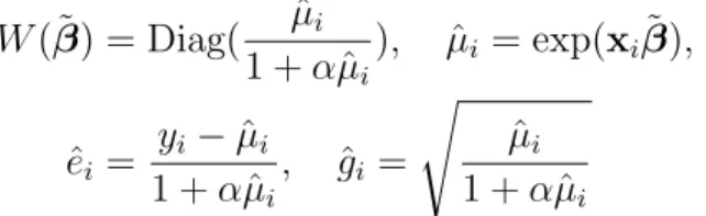
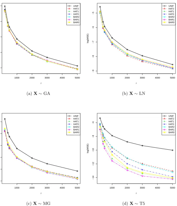
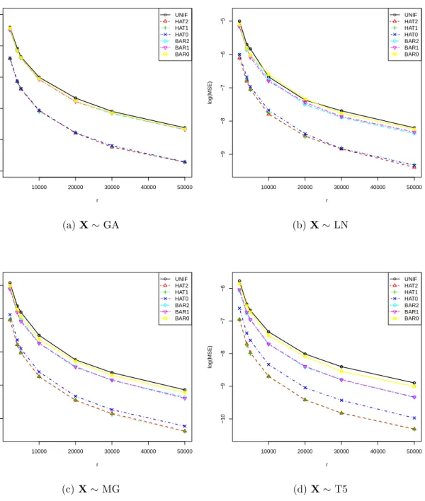
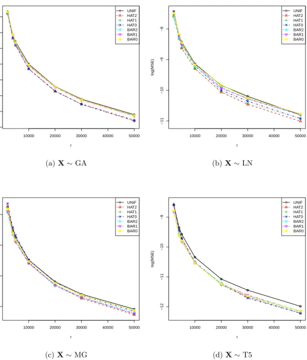
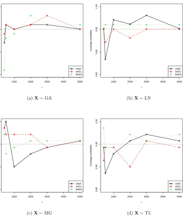
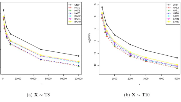
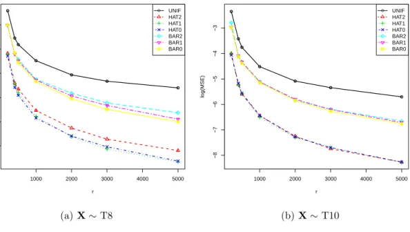
Figure
+7
Related documents
Net positive suction head (NPSH) for positive displacement reciprocating pumps is normally expressed in pressure units (psi, kPa, Bar) since a significant portion of pump NPSHR is
The final regulations provide that appraisal fees incurred by an estate or a trust to determine the fair market value of assets as of the decedent's date of death (or the
___ I understand that volunteer hours submitted for Dental Assistant Training do not qualify for the Volunteer Incentive Program for Red Cross volunteers as it is a
Chapters: Engage with individual leads locally to sell chapter membership; Ensure local programs are aligned with the national message... Membership Marketing
If your bait that you're getting people to send an email to you to become a lead in your autoresponder, is the three biggest mistakes that you're probably making right now in
• Groups who have immigrated to rural or urban New York State or have moved within the state in search of more stable economic, political, and/or social conditions. • Groups
Workplace Safety & Loss Prevention Program List of Private Sector Insurance Company Certified Consultants as of October 1, 2009 3..
Based on the continuing risk of flooding, Aurora has identified the need to mitigate future flood events associated with Westerly Creek in the vicinity of Montview Park from East 23
