Queen’s Economics Department Working Paper No. 1028
Bootstrap Methods in Econometrics
James MacKinnon
Queen’s University
Department of Economics
Queen’s University
94 University Avenue
Kingston, Ontario, Canada
K7L 3N6
Bootstrap Methods in Econometrics
James G. MacKinnon
Department of Economics Queen’s University Kingston, Ontario, Canada
K7L 3N6 [email protected]
http://www.econ.queensu.ca/faculty/mackinnon/
Abstract
There are many bootstrap methods that can be used for econometric analysis. In certain circumstances, such as regression models with independent and identically distributed error terms, appropriately chosen bootstrap methods generally work very well. However, there are many other cases, such as regression models with dependent errors, in which bootstrap methods do not always work well. This paper discusses a large number of bootstrap methods that can be useful in econometrics. Applications to hypothesis testing are emphasized, and simulation results are presented for a few illustrative cases.
Revised, February, 2006; Minor corrections, June, 2006
This research was supported by grants from the Social Sciences and Humanities Re-search Council of Canada. This paper was first presented as a keynote address at the
34th Annual Conference of Economists in Melbourne. I am grateful to an anonymous
1. Introduction
Bootstrap methods involve estimating a model many times using simulated data. Quantities computed from the simulated data are then used to make inferences from the actual data. The term “bootstrap” was coined by Efron (1979), but bootstrap methods did not become popular in econometrics until about ten years ago. One ma-jor reason for their increasing popularity in recent years is the staggering drop in the cost of numerical computation over the past two decades.
Although bootstrapping is quite widely used, it is not always well understood. In practice, bootstrapping is often not as easy to do, and does not work as well, as seems to be widely believed. Although it is common to speak of “the bootstrap,” this is a rather misleading term, because there are actually many different bootstrap methods. Some bootstrap methods are very easy to implement, and some bootstrap methods work extraordinarily well in certain cases. But bootstrap methods do not always work well, and choosing among alternative ones is often not easy.
The next section introduces bootstrap methods in the context of hypothesis testing. Section 3 then discusses methods for bootstrapping regression models. Section 4 deals with bootstrap standard errors, and Section 5 discusses bootstrap confidence intervals. Section 6 deals with bootstrap methods for dependent data, and Section 7 concludes.
2. Hypothesis Testing
Suppose that ˆτ is the realized value of a test statistic τ. If we knew the cumulative
distribution function (CDF) of τ under the null hypothesis, sayF(τ), we would reject
the null hypothesis whenever ˆτ is abnormal in some sense. For a test that rejects in
the upper tail of the distribution, we might choose to calculate a critical value at level
α, say cα, as defined by the equation
1−F(cα) =α. (1)
Then we would reject the null whenever ˆτ > cα. For example, whenF(τ) is the χ2(1)
distribution andα =.05, cα = 3.84.
An alternative approach, which is preferable in most circumstances, is to calculate the
P value, or marginal significance level,
p(ˆτ) = 1−F(ˆτ), (2)
and reject whenever p(ˆτ)< α. It is easy to see that these two procedures must yield
identical inferences, since ˆτ must be greater thancα whenever p(ˆτ) is less than α.
In most cases of interest to econometricians, we do not know F(τ). Until recently,
the usual approach in such cases has been to replace it by an approximate CDF, say
F∞(τ), based on asymptotic theory. This approach works well whenF∞(τ) is a good
approximation toF(τ), but that is by no means always true.
The bootstrap provides another way to approximateF(τ), which may provide a better
to analyze theoretically. It is not even necessary for τ to have a known asymptotic distribution.
In order to perform a bootstrap test, we must generateB bootstrap samples, indexed
by j, that satisfy the null hypothesis. A bootstrap sample is a simulated data set.
The procedure for generating the bootstrap samples, which always involves a random number generator, is called a bootstrap data generating process, or bootstrap DGP. Bootstrap DGPs for regression models will be discussed in the next section.
For each bootstrap sample, we compute a bootstrap test statistic, sayτ∗
j, usually (but
not always) by the same procedure used to calculate ˆτ from the real sample. The
bootstrapP value is then
ˆ p∗(ˆτ) = 1 B B X j=1 I(τj∗ >τˆ), (3)
where I(·) denotes the indicator function, which is equal to 1 when its argument is
true and 0 otherwise. Equation (3) can also be written as ˆ
p∗(ˆτ) = 1−Fˆ∗(ˆτ), (4)
where ˆF∗(τ) denotes the empirical distribution function, or EDF, of the τ∗
j. If we let
the number of bootstrap samples,B, tend to infinity, then ˆF∗(τ) tends to F∗(τ), the
true CDF of theτ∗
j.
The bootstrap P value (4) looks just like the true P value (2), but with the EDF of
the bootstrap distribution, ˆF∗(ˆτ), replacing the unknown CDF F(ˆτ). From this, it
is clear that bootstrap tests will generally not be exact. That is, the probability of
rejecting the null at level α will generally not be equal to α. Most of the problems
with bootstrap tests arise not because ˆF∗(τ) is only an estimate ofF∗(τ) but because
F∗(τ) may not be a good approximation to F(τ).
The bootstrap P value (3) is appropriate if we wish to reject the null hypothesis
whenever ˆτ is sufficiently large and positive. However, for a quantity such as a t
statistic, that can take on either sign, it is generally more appropriate to use either ˆ p∗s(ˆτ) = 1 B B X j=1 I(|τj∗|>|τˆ|), (5) or, alternatively, ˆ p∗ ns(ˆτ) = 2 min µ 1 B B X j=1 I(τ∗ j ≤τˆ), 1 B B X j=1 I(τ∗ j >τˆ) ¶ . (6)
In equation (5), we implicitly assume that the distribution of ˆτ is symmetric around
necessary because there are two tails, and ˆτ could be far out in either tail by chance. Without it, ˆp∗
ns would lie between 0 and 0.5. There is no guarantee that ˆp∗s and p∗ns
will be similar. Indeed, if the mean of the τ∗
j is far from zero, they may be quite
different, and tests based on them may have very different power properties. Unless
the sample size is large, tests based on ˆp∗
s will probably be more reliable, under the
null hypothesis, than tests based on ˆp∗
ns.
2.1 Monte Carlo tests
There is an important special case in which bootstrap tests are exact. For this result to hold, we need two conditions:
1. The test statisticτ is pivotal, which means that its distribution does not depend
on any unknown parameters.
2. The number of bootstrap samplesB is such that α(B+ 1) is an integer, where α
is the level of the test.
When these two conditions hold, a bootstrap test is called a Monte Carlo test. It is
not difficult to see why Monte Carlo tests are exact. By condition 1, ˆτ and the τ∗
j all
come from the same distribution. Now imagine sorting allB+ 1 test statistics. If ˆτ is
one of the largest α(B+ 1) statistics, we reject the null. By condition 2, this happens
with probability α under the null hypothesis. For example, if B = 999 and α = .05,
ˆ
p∗(ˆτ) will be less than .05, and we will consequently reject the null, whenever ˆτ is one
of the 50 largest test statistics.
Monte Carlo tests can be applied to many procedures for testing the specification of linear regression models with fixed regressors and normal errors. What is required is that the test statistic depend only on the least squares residuals and the regressors, and that it not depend on the variance of the error terms. Examples include Durbin-Watson tests and many other tests for serial correlation, tests for ARCH errors and other forms of heteroskedasticity, and Jarque-Bera tests and other tests for skewness and excess kurtosis.
Suppose that X denotes a matrix of fixed regressors and ε a vector of independent,
standard normal random variables. All of the test statistics mentioned in the previous
paragraph depend solely on the OLS residual vectorMXε, whereMX is the projection
matrix I−X(X>X)−1X>, and perhaps on X directly. Since we know X, we can
generate bootstrap test statistics that follow the same distribution as the actual test
statistic under the null. We simply draw the εt as independent standard normal
random variates, regress them on X to obtain the vector of residualsMXε, and then
calculate the test statistic as usual.
When the normality assumption is false, Monte Carlo tests for serial correlation that incorrectly assume it should still be very accurate (although not exact), but Monte Carlo tests for heteroskedasticity may be quite inaccurate. Of course, if there were a reason to assume some distribution other than the normal, the test procedure could
When performing a Monte Carlo test, the penalty for using a small number of bootstrap
samples is loss of power, not loss of exactness. The smallest value of B that can be
used for a test at the .05 level is 19. The smallest value that can be used for a test
at the .01 level is B = 99. Unless computation is very expensive, B = 999 is often a
good choice.
It is possible to perform exact Monte Carlo tests even whenα(B+1) is not an integer —
see Racine and MacKinnon (2004) — but it is only worth the trouble if simulation is very expensive. Other references on Monte Carlo tests include Dwass (1957), in which they were first proposed, J¨ockel (1986) and Davidson and MacKinnon (2000), both of which discuss power loss, Dufour and Khalaf (2001), which is a valuable survey, and Dufour, Khalaf, Bernard, and Genest (2004), which discusses Monte Carlo tests for heteroskedasticity.
2.2 Bootstrap and asymptotic tests
Most test statistics in econometrics are not pivotal. As a consequence, most bootstrap tests are not exact. Nevertheless, there are theoretical reasons to believe that bootstrap tests will often work better than asymptotic tests; see Beran (1988) and Davidson and MacKinnon (1999). For this to be the case, the test statistic must have an asymptotic distribution, but we do not need to know that distribution. Such a test statistic is said to be asymptotically pivotal.
When a test statistic is not pivotal, bootstrap tests are not exact, because F∗(τ)
dif-fers from F(τ). This problem goes away as n → ∞ whenever τ is asymptotically
pivotal, but it does not go away as B → ∞. When F(τ) is not very sensitive to the
values of unknown parameters or the moments of unknown distributions, bootstrap
tests should work well. Conversely, when F(τ) is very sensitive to the values of
un-known parameters or the moments of unun-known distributions, and those parameters or moments are estimated inefficiently and/or with large bias, bootstrap tests may work very badly.
A bootstrap method may have quite different finite-sample properties when it is ap-plied to alternative test statistics for the same hypothesis. As a rule, when we have the opportunity to choose among several asymptotically equivalent test statistics to bootstrap, such as likelihood ratio (LR), Lagrange multiplier (LM), and Wald statis-tics for models estimated by maximum likelihood, we should use the one that is closest to being pivotal. This may or may not be the one that performs most reliably as an asymptotic test.
However, it is important to remember that bootstrap tests are invariant to monotonic
transformations of the test statistic. If τ is a test statistic, and g(τ) is a monotonic
function of it, then a bootstrap test based ong(τ) will yield exactly the same inferences
as a bootstrap test based onτ. The reason for this is easy to see: The position of ˆτ in
the sorted list of ˆτ and the τ∗
j is exactly the same as the position of g(ˆτ) in the sorted
list ofg(ˆτ) and theg(τ∗
j). As an example,F tests and LR tests in linear and nonlinear
different finite-sample properties, they must yield identical results when bootstrapped in the same way.
One important case in which we generally do not know the asymptotic distribution of a test statistic is when that statistic is the maximum of several dependent test statistics. A well-known example is testing for structural change with an unknown break point
(Hansen, 2000). Suppose there are m test statistics, τ1 to τm. Then we simply make
the definition
τmax = max(τ1, . . . , τm) (7)
and treatτmax like any other test statistic for the purpose of bootstrapping. Note that
τmax will be asymptotically pivotal whenever the test statistics τ1 through τm have a
joint asymptotic distribution that is free of unknown parameters.
Whenever we perform two or more tests, it is dangerous to rely on ordinaryP values,
because the probability of obtaining a lowP value by chance increases with the number
of tests we perform. This can be a serious problem when testing model specification and when estimating models with many parameters the significance of which we wish to test. The overall size of such a procedure can be very much larger than the nominal level of each individual test.
By using the bootstrap, it is remarkably easy to obtain an asymptotically valid P
value for the most extreme test statistic actually observed. By analogy with (7), we can define
pmin = min¡p(τ1), . . . , p(τm) ¢
,
wherep(τi) denotes the P value, in most cases computed analytically, for the ith test
statisticτi. Bootstrappingpminis just like bootstrapping τmax defined in (7). Westfall
and Young (1993) provides an extensive discussion of multiple hypothesis testing based on bootstrap methods.
There is a widespread misconception that bootstrap tests are less powerful than other types of tests. Except for the modest loss of power that can arise from using a small
value of B, this is entirely false. Comparing the power of tests that are not exact is
fraught with difficulties; see Horowitz and Savin (2000) and Davidson and MacKinnon (2006a). In general, however, it appears that the powers of asymptotic and bootstrap tests which are based on the same test statistic are very similar when the tests have been properly size-adjusted.
3. Bootstrapping Regression Models
What determines how reliably a bootstrap test performs is how well the bootstrap DGP mimics the features of the true DGP that matter for the distribution of the test statistic. Essentially the same thing can also be said for bootstrap confidence intervals and bootstrap standard errors. In this section, I discuss four different types of bootstrap DGP for regression models with uncorrelated error terms. Models with dependent errors will be discussed in Section 6.
Consider the linear regression model
yt =Xtβ+ut, E(ut|Xt) = 0, E(usut = 0) ∀ s6=t, (8)
where there arenobservations. HereXt is a row vector of observations onkregressors,
andβ is ak--vector. The regressors may include lagged dependent variables, butyt is
not explosive and does not have a unit root.
There are a great many ways to specify bootstrap DGPs for the model (8). Some
require very strong assumptions about the error terms ut, while others require much
weaker ones. In general, making stronger assumptions results in better performance if those assumptions are satisfied, but it leads to asymptotically invalid inferences if they are not. All the methods that will be discussed can also be applied, sometimes with minor changes, to nonlinear regression models.
3.1 The residual bootstrap
If the error terms in (8) are independent and identically distributed with common
varianceσ2, then we can generally make very accurate inferences by using the residual
bootstrap. We do not need to assume that the errors follow the normal distribution or any other known distribution.
The first step in the residual bootstrap is to obtain OLS estimates ˆβ and residuals
ˆ
ut. Unless the quantity to be bootstrapped is invariant to the variance of the error
terms (this is true of test statistics for serial correlation, for example), it is advisable to rescale the residuals so that they have the correct variance. The simplest type of rescaled residual is ¨ ut ≡ µ n n−k ¶1/2 ˆ ut. (9)
The first factor here is the inverse of the square root of the factor by which 1/n
times the sum of squared residuals underestimatesσ2. A somewhat more complicated
method uses the diagonals of the “hat matrix”X(X>X)−1X>to rescale each residual
by a different factor. It may work a bit better than (9) when some observations have high leverage; details are given in Davidson and MacKinnon (2006b).
The residual bootstrap DGP using rescaled residuals generates a typical observation of the bootstrap sample by the equation
y∗
t =Xtβˆ+u∗t, u∗t ∼EDF(¨ut). (10)
The bootstrap errors u∗
t here are said to be “resampled” from the ¨ut. That is, they
are drawn from the empirical distribution function, or EDF, of the ¨ut. This function
assigns probability 1/n to each of the ¨ut. Thus each of the bootstrap error terms can
take onn possible values, namely, the values of the ¨ut, each with probability 1/n.
When the regressors include lagged dependent variables, the bootstrap DGP (10) is
normally implemented recursively, so thaty∗
t depends on its own lagged values. Either
pre-sample values ofyt or drawings from the unconditional distribution of the yt∗ may
3.2 The parametric bootstrap
It may seem remarkable that the residual bootstrap should work at all, let alone that it should work well. The reason it often works well (as we will see in an example below), is that least squares estimates and test statistics are generally not very sensitive to the distribution of the error terms.
Of course, if this distribution is assumed to be known, we can replace (10) by the parametric bootstrap DGP
y∗t =Xtβˆ+ut∗, u∗t ∼NID(0, s2). (11)
Here it is assumed that the errors are normally distributed, and so the bootstrap
error terms are independent normal random variates with variance s2, the usual OLS
estimate of the error variance. Similar methods can be used with any model estimated by maximum likelihood, but their validity generally depends on the strong assumptions inherent in maximum likelihood estimation.
For inferences about regression coefficients, it generally makes very little difference whether we use the residual bootstrap or the parametric bootstrap with normal errors, whether or not the errors are actually normally distributed. However, for inferences about other aspects of a model, such as possible heteroskedasticity, it can make a large difference.
3.3 Restricted versus unrestricted estimates
As described, the residual and parametric bootstraps use unrestricted estimates of β.
This is appropriate in the case of specification tests, such as tests for serial correlation or nonnested hypothesis tests. For example, Davidson and MacKinnon (2002) apply
residual bootstrap methods to theJ test of nonnested hypotheses and find that they
generally work very well. However, using unrestricted estimates is not appropriate if
we are testing a restriction on β.
Both the methods described so far can easily be modified to impose restrictions on
the vector β. In the first step, we simply need to estimate the model under the null
to obtain restricted estimates ˜β. Then we use these estimates instead of ˆβ in the
bootstrap DGP (11). We can resample from either restricted or unrestricted residuals. In most cases, it seems to make little difference which we use.
There are two reasons to use restricted parameter estimates in the bootstrap DGP
when testing restrictions on β. The first reason is that, if we do not do so, the
bootstrap DGP will not satisfy the null hypothesis. If we naively compare ˆτ to the τ∗
j in such a case, the bootstrap test will be grossly lacking in power. It is possible to get
around this problem by changing the null hypothesis used to compute the τ∗
j, as will be discussed below in the context of the pairs bootstrap, but it is preferable to avoid the need to do so.
The second reason for using restricted parameter estimates is that imposing the restric-tions of the null hypothesis yields more efficient estimates of the nuisance parameters
upon which the distribution of the test statistic may depend. This generally makes bootstrap tests more reliable, because the parameters of the bootstrap DGP are es-timated more precisely. For a detailed discussion of how the reliability of bootstrap tests depends on the estimates of nuisance parameters, see Davidson and MacKinnon (1999).
3.4 The wild bootstrap
The residual bootstrap is not valid if the error terms are not independently and iden-tically distributed, but two other commonly used bootstrap methods are valid in this case. The first of these is the “wild bootstrap,” which was proposed by Wu (1986) for regression models with heteroskedastic errors.
For a model like (8) with independent but possibly heteroskedastic errors, the wild bootstrap DGP is
yt∗ =Xtβˆ+f(ˆut)vt∗, (12)
wheref(ˆut) is a transformation of thetthresidual ˆut, andvt∗ is a random variable with
mean 0 and variance 1. One possible choice for f(ˆut) is just ˆut, but a better choice is
f(ˆut) =
ˆ
ut
(1−ht)1/2, (13)
whereht is the tth diagonal of the “hat matrix” that was defined just after (9). When
the f(ˆut) are defined by (13), they would have constant variance if the error terms
were homoskedastic.
There are various ways to specify the distribution of thev∗
t. The simplest, but not the
most popular, is
v∗
t = 1 with probability 12; v∗t =−1 with probability 12. (14)
Thus each bootstrap error term can take on only two possible values. Davidson and Flachaire (2001) have shown that wild bootstrap tests based on (14) usually perform better than wild bootstrap tests which use other distributions when the conditional distribution of the error terms is approximately symmetric. When it is sufficiently asymmetric, however, it may be better to use another two-point distribution, which is the one that is most commonly used in practice:
vt∗ =
(
−(√5−1)/2 with probability (√5 + 1)/(2√5),
(√5 + 1)/2 with probability (√5−1)/(2√5). (15)
The wild bootstrap may seem like a rather strange procedure. When a distribution like (14) or (15) is used, each error term can take on only two possible values, which depend on the size of the residuals. Thus, in certain respects, the bootstrap DGP
cannot possibly resemble the real one. However, the expectation of the square of ˆut is
have about the same variance as the ut. In many cases, this seems to be enough for the wild bootstrap DGP to mimic the essential features of the true DGP.
As with the residual bootstrap, the null hypothesis can, and should, be imposed
when-ever we are using the wild bootstrap to test a hypothesis about β. Although it might
seem that the wild bootstrap works only with cross-section data or static models, variants of it can also be used with dynamic models, provided the error terms are uncorrelated; see Gon¸calves and Kilian (2004).
3.5 The pairs bootstrap
Another method that can accommodate heteroskedasticity is the “pairs bootstrap,” which was proposed by Freedman (1981) and was applied to regressions with instru-mental variables by Freedman (1984) and Freedman and Peters (1984). The idea is to resample the data instead of the residuals. Thus, in the case of the regression model
(8), we resample from the matrix [y X] with typical row [yt Xt]. Each observation
of the bootstrap sample is [y∗
t Xt∗], a randomly chosen row from [y X]. This method
is called the pairs (or pairwise) bootstrap because the dependent variable y∗
t and the
independent variables X∗
t are always selected in pairs.
Unlike the residual and wild bootstraps, the pairs bootstrap does not condition on X. Instead, each bootstrap sample has a different X∗ matrix. This method
implic-itly assumes that each observation [yt Xt] is an independent random drawing from a
multivariate distribution. It does not require that the error terms be homoskedastic, and it even works for dynamic models if we treat lagged dependent variables like any
other element ofXt.
In the case of multivariate models, we can combine the pairs and residual bootstraps. We organize the residuals into a matrix and then apply the pairs bootstrap to its rows, adding the bootstrap error terms so generated to the appropriate fitted values to yield the bootstrap data. This method preserves the cross-equation correlations of the residuals without imposing any distributional assumptions on the bootstrap error terms.
The pairs bootstrap is very easy to implement, and it can be applied to an enormous range of models. However, it suffers from two major deficiencies. The first of these is
that the bootstrap DGP does not impose any restrictions onβ. If we are testing such
restrictions, as opposed to estimating standard errors or forming confidence intervals, we need to modify the bootstrap test statistic so that it is testing something which
is true in the bootstrap DGP. Suppose the actual test statistic takes the form of a t
statistic for the hypothesis thatβ =β0:
τ = βˆ−β
0
Here ˆβ is the unrestricted estimate of the parameter β that is being tested, ands( ˆβ) is its standard error. Then, for bootstrap testing to be valid, we must use the bootstrap test statistic τj∗ = βˆ ∗ j −βˆ s( ˆβ∗ j) . (17) Here ˆβ∗
j is the estimate of β from the jth bootstrap sample, and s( ˆβj∗) is its standard
error, calculated using the bootstrap sample by whatever procedure was employed to
calculate s( ˆβ) using the actual sample. Since the estimate of β from the bootstrap
samples should, on average, be equal to ˆβ, at least asymptotically, the null hypothesis
tested byτ∗
j is “true” for the pairs bootstrap DGP.
The other deficiency of the pairs bootstrap is that, compared to the residual bootstrap (when it is valid) and to the wild bootstrap, the pairs bootstrap generally does not yield very accurate results. This is primarily because it does not condition on the
actual X matrix. In the next subsection, we will examine a case in which the pairs
bootstrap does not work particularly well. 3.6 A comparison of several methods
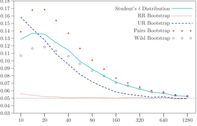
To demonstrate how well, or how badly, various bootstrap procedures perform, it is necessary to perform a simulation experiment. As an illustration, consider testing the
null hypothesis thatβ2 = 0.9 in the autoregressive model
yt =β1+β2yt−1+ut, ut ∼NID(0, σ2). (18)
Standard tests are not exact here, because ˆβ2, the OLS estimate of β2, is biased. All
tests are based on the usualt statistic
τ = β2ˆ −0.9
s( ˆβ2) . (19)
It may seem odd that the null hypothesis is thatβ2 = 0.9 rather thanβ2 = 0 orβ2 = 1.
The reason for not examining tests forβ2 = 0 is that asymptotic methods work pretty
well for that case, and there is not much to be gained by using the bootstrap. The
reason for not examining tests for β2 = 1 is that the asymptotic theory changes
drastically when there is a unit root. The values ofβ1 andσ seem to have only a small
effect on the results; in the experiments, these values were β1 = 1 andσ = 1.
The experiments deal with five methods of inference. The first uses the Student’s t
distribution, which is valid only asymptotically in this case. The second is the residual bootstrap using restricted estimates and restricted residuals rescaled using (9), called the “RR bootstrap” for short. The third is the residual bootstrap using unrestricted estimates and unrestricted rescaled residuals, called the “UR bootstrap” for short. The fourth is the pairs bootstrap, and the fifth is the wild bootstrap using the two-point distribution (14) and residuals rescaled by (13).
Each experiment had 100,000 replications, with B = 399. This is a smaller value of
B than should generally be used in practice, but in a simulation experiment with a
large number of replications, the randomness due to B being small tends to average
out across the replications. Thus, when we are studying the properties of a bootstrap
test under the null hypothesis, there is generally no reason to use a large value of B.
Experiments were performed for each of the following sample sizes: 10, 14, 20, 28, 40, 56, 80, 113, 160, 226, 320, 452, 640, 905, and 1280. Each of these is larger than its predecessor by approximately the square root of 2.
[Figure 1 about here]
We can see from Figure 1 that inference based on the t distribution is seriously
un-reliable. It improves as n increases, but it is by no means totally reliable even for
n= 1280. In contrast, inference based on the RR bootstrap is extraordinarily reliable.
Only for very small sample sizes does it lead to nonnegligible rates of overrejection. In contrast, the other four bootstrap methods do not work particularly well. The pairs
bootstrap always performs worse than thetdistribution. The wild bootstrap generally
outperforms the t distribution, but only modestly so. The UR bootstrap is the worst
method for n= 10, and it always performs badly for small sample sizes. However, it
improves more rapidly than any of the others asnincreases, and it appears to perform
just as well as the RR bootstrap for large sample sizes.
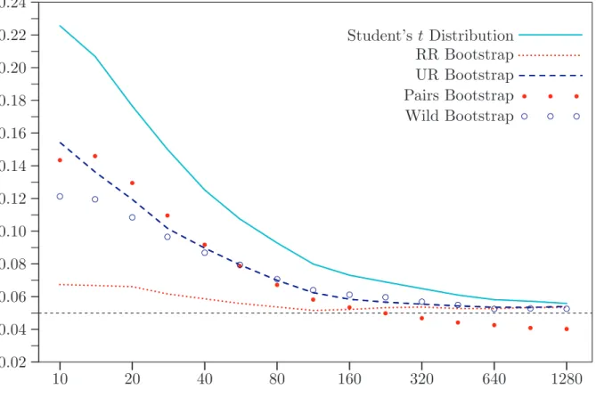
This example may be unfair to the wild and pairs bootstraps, because the error terms are independent and identically distributed. Suppose instead they follow the
GARCH(1,1) process
σ2
t ≡E(u2t) =α0+α1u2t−1+δ1σt2−1, (20)
with α0 = 0.1, α1 = 0.1, and δ1 = 0.8. Instead of using the ordinary t statistic (19),
we now use the heteroskedasticity-robust pseudo-t statistic
ˆ
β2−0.9
sh( ˆβ2)
, (21)
wheresh( ˆβ2) is a heteroskedasticity-consistent standard error. There are several ways
to calculate such a standard error. The one used in the experiments is based on the
HCCME known as HC2, which will be described in the next section.
[Figure 2 about here]
Figure 2 shows the results of this second set of experiments. All the bootstrap methods
now reject less frequently than thetdistribution for all sample sizes. However, all but
the RR bootstrap perform quite poorly when n is small. The wild bootstrap seems
to perform best when n is very large, which is in accord with theory. However, the
pairs bootstrap actually underrejects in this case, which is somewhat worrying. The surprisingly good performance of the RR bootstrap, even though it does not allow for
heteroskedasticity, is presumably because the bias in ˆβ2 is much more important than the heteroskedasticity of the error terms.
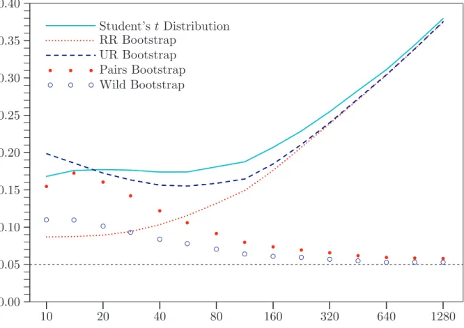
[Figure 3 about here]
Figure 3 shows what happens when the ordinary t statistic (19) is used and the error
terms follow the GARCH(1,1) process (20). This test statistic is not asymptotically
valid in the presence of heteroskedasticity. Not surprisingly, the t distribution and
the RR and UR bootstraps work terribly, and their performance deteriorates as n
increases. However, the wild bootstrap performs about as well as it did when the test statistic was (21), and the pairs bootstrap also performs reasonably well for large sample sizes. In this case, the ability of the wild and pairs bootstraps to mimic the heteroskedasticity in the data is evidently critical.
4. Bootstrap Standard Errors
The bootstrap was originally proposed as a method for computing standard errors; see Efron (1979, 1982). It can be valuable for this purpose when other methods are computationally difficult, are unreliable, or are not available at all.
If ˆθ is a parameter estimate, ˆθ∗
j is the corresponding estimate for the jth bootstrap
replication, and ¯θ∗ is the mean of the ˆθ∗
j, then the bootstrap standard error is
s∗(ˆθ) = µ 1 B−1 B X j=1 (ˆθ∗j −θ¯∗)2 ¶1/2 . (22)
This is simply the sample standard deviation of the ˆθ∗
j. We can use s∗(ˆθ) in the
same way as we would use any other asymptotically valid standard error to construct asymptotic confidence intervals or perform asymptotic tests.
Although there are many situations in which bootstrap standard errors are useful (we will encounter one in the next section), there are others in which they provide no advantage. In the context of ordinary least squares, for example, it makes absolutely no sense to use bootstrap standard errors.
There are two widely-used estimators for the covariance matrix of the OLS parameter
vector ˆβ in the model (8) when the error terms are independent. The best-known,
which is valid when the error terms are homoskedastic, is
d
Var( ˆβ) =s2(X>X)−1. (23)
Under heteroskedasticity of unknown form, this estimator is invalid. Instead, we would use a heteroskedasticity-consistent covariance matrix estimator, or HCCME, of the form
d
Varh( ˆβ) = (X>X)−1X>ΩX(Xˆ >X)−1, (24)
where ˆΩ is ann×ndiagonal matrix with diagonal elements equal to the squared
of least squares residuals to be too small. The HC2 variant of (24) divides each of the
squared residuals by 1−ht, where ht is a diagonal element of the “hat matrix” that
was defined just after (9); see Davidson and MacKinnon (2004, Chapter 5). Whatever the bootstrap DGP, the bootstrap covariance matrix is
d Var∗( ˆβ) = 1 B−1 B X j=1 ( ˆβ∗ j −β¯∗)( ˆβj∗−β¯∗)>, (25)
where the notation should be obvious; compare (22). For a residual bootstrap DGP
like (10), it can be shown that, as n andB become large, (25) tends to
σ∗2(X>X)−1, (26)
where σ2
∗ is the average variance of the bootstrap error terms. This matrix tends to
the same limit as (23). Thus, in this case, the bootstrap covariance matrix (25) is valid if the errors are independent and homoskedastic, but not otherwise.
In contrast, for the wild bootstrap, the bootstrap covariance matrix (25) is approxi-mately equal to the matrix
1 B B X j=1 (Xj>Xj)−1Xj>u∗ju∗j>Xj(Xj>Xj)−1, (27) where u∗
j is the vector of bootstrap error terms for the jth bootstrap sample. This
looks a lot like the HCCME (24). The matrix in the middle here is approximately
equal to X>ΩX. Thus, forˆ B and n reasonably large, we would expect (27) to be
very similar to the HCCME (24). A similar argument can be applied to the pairs bootstrap; see Flachaire (2002).
We have seen that, for a linear regression model, there is nothing to be gained by using a bootstrap covariance matrix instead of a conventional one like (23) or (24). However, when convenient analytical results like these are not available, bootstrap covariance matrices and standard errors can be very useful.
5. Bootstrap Confidence Intervals
There is an extensive literature, mainly by statisticians, on the numerous ways to construct bootstrap confidence intervals. Davison and Hinkley (1997) provides a very good introduction to this literature, which is much too large to discuss in any detail. 5.1 Simple bootstrap confidence intervals
The simplest approach is to calculate the bootstrap standard error (22) and use it to construct a confidence interval based on the normal distribution:
£ˆ
Here z1−α/2 denotes the 1 −α/2 quantile of the standard normal distribution. If
α = .05, this is equal to 1.96. There is no theoretical reason to believe that the
“simple bootstrap” interval (28) will work any better, or any worse, than a similar interval based purely on asymptotic theory. However, it can be used when there is no way to calculate a standard error analytically or when asymptotic standard errors are
unreliable. Another advantage of (28) is that the number of bootstrap samples, B,
does not have to be very large.
The simple bootstrap interval can be modified so that it is centered on a bias-corrected
estimate of θ. We simply replace ˆθ in (28) by
ˇ
θ = ˆθ−(¯θ∗−θˆ) = 2 ˆθ−θ¯∗; (29)
recall that ¯θ∗ is the sample mean of the θ∗
j. In (29), we use the difference between ¯θ∗
and ˆθto estimate the bias, and then we subtract the estimated bias. The bias-corrected
estimator ˇθ almost always has a larger standard error than ˆθ, but bias correction can
be helpful if the bias is severe and does not depend strongly onθ; see MacKinnon and
Smith (1998).
5.2 Percentilet confidence intervals
A method that has better properties than the simple bootstrap interval, at least in
theory, is the “percentile t” method, also called “bootstrap t” and “Studentized
boot-strap,” which has been advocated by Hall (1992). A percentile t confidence interval
for θ at level 1−α is £
ˆ
θ−s(ˆθ)t∗1−α/2, θˆ−ˆs(ˆθ)t∗α/2¤, (30) wheres(ˆθ) is the standard error of ˆθ, andt∗
δ is theδquantile of the bootstraptstatistics
t∗j = θˆ ∗ j −θˆ s(ˆθ∗ j) . (31)
For example, if α = .05 and B = 999, t∗
1−α/2 will be number 975, and t∗α/2 will be
number 25, in the sorted list of the t∗
j. The use of B= 999 in this example is not an
accident. A fairly large value of B is needed if the quantiles of the distribution of the
t∗
j are to be estimated accurately, and, as with bootstrap tests, it is desirable for B to
be chosen in such a way that α(B+ 1) is an integer.
The interval (30) looks very much like an ordinary confidence interval based on
invert-ing a t statistic, except that quantiles of the bootstrap distribution of the t∗
j are used
instead of quantiles of the Student’s t distribution. Because of this, the percentile
t method implicitly performs a sort of bias correction. When the median of the t∗
j
is positive (negative), the percentile t interval tends to be shifted to the left (right)
relative to an asymptotic interval based on the normal or Student’st distributions.
In theory, percentilet confidence intervals achieve “higher-order accuracy” relative to
at which the error in coverage probability declines as n increases is faster than it is
for asymptotic methods. However, as we will see in the next subsection, percentile t
intervals do not always perform well in practice; see also MacKinnon (2002).
The percentile t method evidently cannot be used if s(ˆθ) cannot be calculated. It
should not be used if s(ˆθ) is unreliable or strongly dependent on ˆθ, since its excellent
theoretical properties do not seem to apply in practice in such cases. This method
seems to be particularly useful when the t statistic for ˆθ to equal its true value is not
symmetrically distributed around zero, but s2(ˆθ) is a reliable estimator of Var(ˆθ).
5.3 Comparing bootstrap confidence intervals
Here we perform a simulation to illustrate the fact that bootstrap confidence intervals
do not always work particularly well. Suppose that yt, t= 1, . . . , n, are drawings from
a distribution F(y). We want to form confidence intervals for some of the quantiles
of F(y). If qα is the true α quantile, and ˆqα is the corresponding estimate, then
asymptotic theory tells us that
Var(ˆqα)=a
α(1−α)
nf2(q
α) . (32)
Here f(qα) is f(y), the density ofy, evaluated atqα. In practice, we replace f(qα) by
a kernel density estimate ˆf(ˆqα) so as to obtain the standard error estimate
s(ˆqα) = µ α(1−α) nfˆ2(ˆq α) ¶1/2 . (33)
Thus the 0.95 asymptotic confidence interval is equal to
£
ˆ
qα −1.96s(ˆqα), qˆα + 1.96s(ˆqα) ¤
. (34)
The simplest bootstrap procedure is just to resample the data, calculate the desired quantile(s) of each bootstrap sample, and then use equation (22) to estimate the bootstrap standard error. This yields the 0.95 simple bootstrap interval
£
ˆ
qα−1.96s∗(ˆqα), qˆα + 1.96s∗(ˆqα) ¤
. (35)
We can also use the percentile t method. This is much more expensive, because it
requires kernel estimation for the actual sample and for every bootstrap sample.
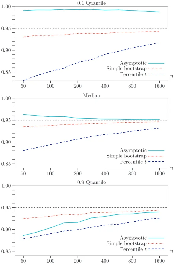
In the experiments,F(y) wasχ2(3), which is severely skewed to the right,B was 999,
and α = 0.1,0.2, . . . ,0.9. The sample size n varied from 50 to 1600 by factors of √2. A very standard method of kernel estimation was employed. It used a Gaussian kernel
with bandwidth equal to 1.059n−1/5 times the sample standard deviation of the y
t. There were 100,000 replications for each sample size.
Figure 4 shows the coverage frequency of three different confidence intervals for the 0.1 quantile, the 0.5 quantile (the median), and the 0.9 quantile. The coverage frequency is the proportion of the time that the interval includes the true value of the quantile. Ideally, it should be 0.95 here. The simulation results are not in accord with stan-dard bootstrap theory. The asymptotic interval sometimes overcovers and sometimes undercovers, while both bootstrap intervals always undercover. The simple bootstrap interval, which is conceptually the easiest to calculate, clearly performs best for both the 0.1 and 0.9 quantiles. The asymptotic interval performs best for the median. In
contrast, the percentile t interval, which theory seems to recommend, performs least
well in almost every case. This is probably because the estimated standard errors, given in equation (33), are not particularly reliable and are not independent of the quantile estimates.
6. Bootstrap DGPs for Dependent Data
All of the bootstrap DGPs that have been discussed so far treat the error terms (or the data, in the case of the pairs bootstrap) as independent. When that is not the case, these methods are not appropriate. In particular, resampling (whether of residuals or data) breaks up whatever dependence there may be and is therefore unsuitable for use when there is dependence.
Numerous bootstrap DGPs for dependent data have been proposed. The two most popular approaches are the “sieve bootstrap” and the “block bootstrap.” The former attempts to model the dependence using a parametric model. The latter resamples blocks of consecutive observations instead of individual observations. Each of these methods has a great many variants, and the discussion here is necessarily quite
su-perficial. Recent surveys of bootstrap methods for time-series data include B¨uhlmann
(2002), Horowitz (2003), Politis (2003), and H¨ardle, Horowitz, and Kreiss (2003). 6.1 The sieve bootstrap
Suppose that the error terms ut in a regression model, which for simplicity we may
assume to be the linear regression model (8), follow an unknown, stationary process with homoskedastic innovations. The sieve bootstrap attempts to approximate this
process, generally by using an AR(p) process with p chosen either by some sort of
model selection criterion or by sequential testing.
The first step is to estimate the model (8), preferably imposing the null hypothesis
if one is to be tested, so as to obtain residuals ˆut. The next step is to estimate the
AR(p) model ˆ ut = p X i=1 ρiuˆt−i+εt (36)
for several values of p and choose the best one. This may be done in a number of
ways. Since OLS estimation does not ensure that the estimated model is stationary, it may be advisable to use another estimation method, such as full maximum likelihood
or the Yule-Walker equations, so as to ensure stationarity. See Brockwell and Davis (1998) or Shumway and Stoffer (2000) for discussions of these methods.
After p has been chosen and the preferred version of (36) estimated, the bootstrap
error terms are generated recursively by the equation
u∗ t = p X i=1 ˆ ρiu∗t−i+εt∗, t=−m, . . . ,0,1, . . . , n, (37)
where the ˆρiare the estimated parameters, and theε∗t are resampled from the (possibly
rescaled) residuals. Here m is a somewhat arbitrary number, such as 100, chosen so
that the process can be allowed to run for some time before the sample period starts.
We set the initial values of u∗
t−i to zero and discard the u∗t for t < 1. The final step is to generate the bootstrap data by the equation
yt∗ =Xtβˆ+u∗t, (38)
where ˆβmay be estimated in various ways. If restrictions are being tested, they should
always be imposed, but this is not done when constructing confidence intervals. OLS estimates are typically used, but more efficient estimates can often be obtained by using GLS based on the covariance matrix implied by (37). Obviously, whatever estimates are used must be consistent under the null hypothesis.
The sieve bootstrap is somewhat restrictive, because it assumes that the innovations,
theεt, are independent and identically distributed. This rules out GARCH models and
other forms of conditional heteroskedasticity. Moreover, as we will see below, an AR(p)
model with a reasonable value of p does not provide a good approximation to every
stationary, stochastic process. Nevertheless, the sieve bootstrap is quite popular. It has recently been applied to Dickey-Fuller unit root testing by Park (2003) and Chang and Park (2003), and it seems to work quite well in many cases.
6.2 Block bootstrap methods
Block bootstrap methods, originally proposed by K¨unsch (1989), divide the quantities
that are being resampled, which might be either rescaled residuals or [y,X] pairs, into
blocks of b consecutive observations. The blocks, which may be either overlapping or
nonoverlapping and may be either fixed or variable in length, are then resampled. It appears that the best approach is to use overlapping blocks of fixed length; see Lahiri (1999). This is called the “moving-block bootstrap.”
For the moving-block bootstrap, there are n−b+ 1 blocks. The first contains
obser-vations 1 through b, the second contains observations 2 through b+ 1, and the last
contains observationsn−b+ 1 through n. Each bootstrap sample is then constructed
by resampling from these overlapping blocks. Unlessn/b is an integer, one or more of
the blocks will have to be truncated to form a sample of length n.
The choice of b is critical. In theory, it must be allowed to increase as n increases,
sizes are generally fixed, it is not clear what this means in practice. If the blocks are too short, the bootstrap samples cannot possibly mimic the original sample, because the dependence is broken whenever we start a new block. However, if the blocks are too long, the bootstrap samples are not random enough. In many cases, it is only
when the sample size is quite large that is it possible to choose b so that the blocks
are neither too short nor too long.
The “block-of-blocks” bootstrap (Politis and Romano, 1992) is the analog of the pairs bootstrap for dynamic models. Consider the dynamic regression model
yt =Xtβ+γ yt−1+ut, ut ∼IID(0, σ2). (39)
If we define
Zt ≡[yt, yt−1,Xt], (40)
we can construct n−b+ 1 overlapping blocks as
Z1. . .Zb, Z2. . .Zb+1, . . . ,Zn−b+1. . .Zn. (41) These are then resampled in the usual way.
The advantages of the block-of-blocks bootstrap are that it can be used with almost any sort of dynamic model and that it can handle heteroskedasticity as well as serial correlation. However, its finite-sample performance is often not very good. Moreover, since it does not impose the null hypothesis, any test statistic must be adjusted so that it is testing a hypothesis that is true for the bootstrap DGP. Ideally, this adjustment should take account of the fact that, because of the overlapping blocks, not all obser-vations appear with equal frequency in the bootstrap samples. See Horowitz, Lobato, Nankervis, and Savin (2006).
The theoretical properties of block bootstrap methods are not particularly good. When
used for testing and for construction of percentiletconfidence intervals, they frequently
offer higher-order accuracy than asymptotic methods. However, the rate of improve-ment is generally quite small; see Hall, Horowitz, and Jing (1995) and Andrews (2002, 2004). Two other recent theoretical papers which focus on different aspects of block bootstrap methods are Gon¸calves and White (2004, 2005).
6.3 Example: a unit root test
The asymptotic distributions of many unit root tests do not depend on the process that generates the error terms, but the finite-sample distributions do. Consider an
augmented Dickey-Fuller test for a time series with tth observation y
t to have a unit
root. One popular version of such a test is the t statistic for β1 = 0 in the regression
∆yt =β0+β1yt−1+
p X j=1
Theplags of ∆yt−j are added to account for serial correlation in the error terms. The
value of p can be chosen in a number of different ways, which substantially affect the
finite-sample properties of the resulting tests. These include model selection criteria, such as AIC and BIC, and various sequential testing schemes; see, among others, Ng and Perron (2001).
In order to bootstrap this test, we first run the regression under the null thatβ1 = 0
and then generate bootstrap samples that satisfy the null. There are several ways in which to do this, which lead to bootstrap DGPs that can have quite different finite-sample properties.
For the sieve bootstrap, we first regress ∆yt on a constant and a number of lags of
∆yt, obtaining coefficients ˆρi and residuals ˆεt. We then generate data according to
the equation yt∗ =y∗t−1+ q X i=1 ˆ ρi∆yt∗−i+ε∗t, t=−m, . . . ,0,1, . . . , n,
setting the initial values of y∗
t−i to zero. The ε∗t are resampled from the rescaled ˆεt.
Like the value of p in equation (42), the number of lags, q, can be chosen in various
ways. In practice, q may or may not equal p. The details of how q is chosen may
substantially affect the performance of the bootstrap DGP in finite samples.
For the moving-block bootstrap, there are no parameters to estimate, because we are not attempting to estimate the process for the error terms and, under the null
hypothe-sis,β0 = 0 andβ1 = 1. The residuals under the null are just ˆut = ∆yt−
Pn
t=1(1/n)∆yt, where the second term is needed to ensure that they have mean zero. We resample the
bootstrap errorsu∗
t from overlapping blocks of the ˆut and then generate the bootstrap
data according to the random walk y∗
t =y∗t−1+u∗t. The easiest way to deal with the
initial observations is to start the process at zero and generate n+m observations,
discarding the firstm of them.
If we knew that the error terms followed a particular process, we could estimate it and use a semiparametric bootstrap. For example, if they followed an MA(1) process, we could estimate the model
∆yt =β0+εt +αεt−1, εt ∼IID(0, σ2), (43)
and generate the bootstrap data according to the equation
y∗
t =y∗t−1+ε∗t + ˆαε∗t−1,
where theε∗
t are resampled from rescaled and recentered ˆεt.
For purposes of illustration, I performed a number of experiments in which there were 50 observations and the errors actually followed the MA(1) process (43). There were
100,000 replications for each of 39 values ofα from −0.95 to 0.95 at intervals of 0.05.
to be between 4 and 12. This selection procedure was repeated for each bootstrap sample. I used three bootstrap DGPs. The first was a moving-block bootstrap with
block length 12. The second was a sieve bootstrap with q restricted to lie between
4 and 12 and chosen by the AIC. The third was a semiparametric bootstrap based on (43). Readers may well feel that it is cheating to use the last of these procedures, since practitioners will rarely be confident that the data actually come from an MA(1) process.
[Figure 5 about here]
The results of these experiments are shown in Figure 5. It can be seen that the “asymptotic” test always overrejects, although the overrejection is only severe for
large, negative values of α. The results termed “asymptotic” actually use a
finite-sample critical value, −2.9212, that would be valid if there were no serial correlation
and no lags of ∆yt in the test regression. It was taken from MacKinnon (1996). Using
the genuine asymptotic critical value, −2.8614, would have resulted in slightly higher
rejection frequencies.
All three bootstrap methods work remarkably well for α > 0, but all three work
poorly for α <−0.9. Not surprisingly, the semiparametric procedure generally works
best, but even it overrejects quite noticeably for large, negative values of α. This
presumably happens because the estimate of α is biased upwards in this case, so
that the bootstrap DGP fails to mimic the true DGP sufficiently well. The sieve and moving-block bootstraps overreject much more severely. In the case of the sieve bootstrap, this reflects the fact that even a fairly high-order AR process does not do a very good job of mimicking an MA(1) process with a large, negative coefficient. Interestingly, even though the moving-block bootstrap overrejects severely for large,
negative values ofα, it underrejects quite noticeably for smaller, negative values.
This example illustrates the facts that bootstrap methods may or may not yield ac-curate inferences, and that different bootstrap methods may perform quite differently. It suggests that bootstrap methods should be used with considerable caution when performing unit root and related tests.
7. Conclusions
It is very misleading to talk about “the bootstrap,” because there are actually many different bootstrap methods. Deciding what sort of bootstrap DGP to use in any given situation is the first, and often the hardest, thing that an applied econometrician must do. Conditional on the choice of bootstrap DGP, there are then a number of other substantive decisions to be made.
In the case of hypothesis testing, it is almost always desirable to impose the null hypothesis on the bootstrap DGP, but it may not be feasible to do so. When it is not, we have to change the null hypothesis for the bootstrap samples so that whatever is being tested is “true” for the bootstrap data. There is often more than one statistic that could be bootstrapped, and we have to choose among them. For tests based on
signed statistics, such as t statistics, we may or may not wish to assume symmetry
when calculating P values.
For confidence intervals, the number of options is bewildering. We can use asymptotic intervals constructed using bootstrap standard errors, which may or may not
incor-porate bias correction. We can use percentile t intervals based on various types of
standard errors, which may or may not have symmetry imposed on them. We can also use a number of methods that were not discussed in this paper, including primitive
ones like the “percentile method” and more sophisticated ones like the BCa method;
see Efron and Tibshirani (1993) and Davison and Hinkley (1997).
Whatever bootstrap methods we choose to use, it is always important to make it clear precisely what was done whenever we report the results of empirical work. Simply
saying that something is a “bootstrap standard error,” a “bootstrap P value,” or a
“bootstrap confidence interval” provides the reader with grossly insufficient informa-tion. We need to make it clear exactly how the bootstrap data were generated and what procedures were then used to calculate the quantities of interest.
References
Andrews, D. W. K. (2002). “Higher-order improvements of a computationally attractive k-step bootstrap for extremum estimators,” Econometrica, 70, 119–162.
Andrews, D. W. K. (2004). “The block-block bootstrap: Improved asymptotic refinements,” Econometrica, 72, 673–700.
Beran, R. (1988). “Prepivoting test statistics: A bootstrap view of asymptotic refinements,” Journal of the American Statistical Association, 83, 687–697.
Brockwell, P. J., and R. A. Davis (1998).Time Series: Theory and Methods, Second Edition, New York, Springer-Verlag.
B¨uhlmann, P. (2002). “Bootstraps for time series,” Statistical Science, 17, 52–72.
Chang, Y., and J. Y. Park (2003). “A sieve bootstrap for the test of a unit root,” Journal of Time Series Analysis, 24, 379–400.
Davidson, R., and E. Flachaire (2001). “The wild bootstrap, tamed at last,” GREQAM Document de Travail 99A32, revised.
Davidson, R., and J. G. MacKinnon (1999). “The size distortion of bootstrap tests,” Econo-metric Theory, 15, 361–376.
Davidson, R., and J. G. MacKinnon (2000). “Bootstrap tests: How many bootstraps?” Econometric Reviews, 19, 55–68.
Davidson, R., and J. G. MacKinnon (2002). “BootstrapJ tests of nonnested linear regression models,”Journal of Econometrics, 109, 167–193.
Davidson, R., and J. G. MacKinnon (2004). Econometric Theory and Methods, New York, Oxford University Press.
Davidson, R., and J. G. MacKinnon (2006a). “The power of bootstrap and asymptotic tests,” Journal of Econometrics, forthcoming.
Davidson, R., and J. G. MacKinnon (2006b). “Bootstrap methods in econometrics,” Chapter 23 in Palgrave Handbook of Econometrics: Volume 1 Theoretical Econometrics, ed. K. Patterson and T. C. Mills, Basingstoke, Palgrave Macmillan, 812–838.
Davison, A. C., and D. V. Hinkley (1997).Bootstrap Methods and Their Application, Cam-bridge, Cambridge University Press.
Dufour, J.-M., and L. Khalaf (2001). “Monte Carlo test methods in econometrics,” Chapter 23 inA Companion to Econometric Theory, ed. B. Baltagi, Oxford, Blackwell Publishers, 494–519.
Dufour, J.-M., L. Khalaf, J.-T. Bernard, and I. Genest (2004). “Simulation-based finite-sample tests for heteroskedasticity and ARCH effects,”Journal of Econometrics, 122, 317– 347.
Dwass, M. (1957). “Modified randomization tests for nonparametric hypotheses,” Annals of Mathematical Statistics, 28, 181–187.
Efron, B. (1979). “Bootstrap methods: Another look at the jackknife,” Annals of Statistics, 7, 1–26.
Efron, B. (1982). The Jackknife, the Bootstrap and Other Resampling Plans, Philadelphia, Society for Industrial and Applied Mathematics.
Efron, B., and R. J. Tibshirani (1993).An Introduction to the Bootstrap, New York, Chapman and Hall.
Flachaire, E., (2002). “Bootstrapping heteroskedasticity consistent covariance matrix estima-tor,”Computational Statistics, 17, 501–506.
Freedman, D. A. (1981). “Bootstrapping regression models,” Annals of Statistics, 9, 1218– 1228.
Freedman, D. A. (1984). “On bootstrapping stationary two-stage least-squares estimates in stationary linear models,”Annals of Statistics, 12, 827–842.
Freedman, D. A., and S. C. Peters (1984). “Bootstrapping an econometric model: Some empirical results,”Journal of Business and Economic Statistics, 2, 150–158.
Gon¸calves, S., and L. Kilian (2004). “Bootstrapping autoregressions with heteroskedasticity of unknown form,” Journal of Econometrics, 123, 89–120.
Gon¸calves, S., and H. White (2004). “Maximum likelihood and the bootstrap for dynamic nonlinear models,”Journal of Econometrics, 119, 199–219.
Gon¸calves, S., and H. White (2005). “Bootstrap standard error estimates for linear regression” Journal of the American Statistical Association, 120, 970–979.
Hall, P. (1992).The Bootstrap and Edgeworth Expansion, New York, Springer-Verlag. Hall, P., J. L. Horowitz, and B. Y. Jing (1995). “On blocking rules for the bootstrap with
dependent data,” Biometrika, 82, 561–574.
Hansen, B. E. (2000). “Testing for structual change in conditional models,”Journal of Econo-metrics, 97, 93–115.
H¨ardle, W., J. L. Horowitz, and J.-P. Kreiss (2003). “Bootstrap methods for time series,” International Statistical Review, 71, 435–459.
Horowitz, J. L. (2003). “The bootstrap in econometrics,” Statistical Science, 18, 211–218. Horowitz, J. L., and N. E. Savin (2000). “Empirically relevant critical values for hypothesis
tests,”Journal of Econometrics, 95, 375–389.
Horowitz, J. L., I. L. Lobato, J. C. Nankervis, and N. E. Savin (2006). “Bootstrapping the Box-Pierce Q test: A robust test of uncorrelatedness,”Journal of Econometrics, forthcoming. J¨ockel, K.-H. (1986). “Finite sample properties and asymptotic efficiency of Monte Carlo
tests,”Annals of Statistics, 14, 336–347.
K¨unsch, H. R. (1989). “The jackknife and the bootstrap for general stationary observations,” Annals of Statistics, 17, 1217–1241.
Lahiri, S. N. (1999). “Theoretical comparisons of block bootstrap methods,” Annals of Stat-istics, 27, 386–404.
MacKinnon, J. G. (1996). “Numerical distribution functions for unit root and cointegration tests,”Journal of Applied Econometrics, 11, 601–618.
MacKinnon, J. G. (2002). “Bootstrap inference in econometrics,”Canadian Journal of Econ-omics, 35, 615–645.
MacKinnon, J. G., and A. A. Smith (1998). “Approximate bias correction in econometrics,” Journal of Econometrics, 85, 205–230.
Ng, S., and P. Perron (2001). “Lag length selection and the construction of unit root tests with good size and power,”Econometrica, 69, 1519–1554.
Park, J. Y. (2003). “Bootstrap unit root tests,”Econometrica, 71, 1845–1895.
Politis, D. N., and J. P. Romano (1992). “General resampling scheme for triangular arrays of α-mixing random variables with application to the problem of spectral density estimation,” Annals of Statistics, 20, 1985–2007.
Politis, D. N. (2003). “The impact of bootstrap methods on time series analysis,”Statistical Science, 18, 219–230.
Racine, J. and J. G. MacKinnon (2004). “Simulation-based tests that can use any number of simulations,” Queen’s Economics Department Working Paper Number 1027.
Shumway, R. H. and S. S. Stoffer (2000). Time Series Analysis and Its Applications, New York, Springer-Verlag.
Westfall, P. H., and S. Young (1993).Resampling-Based Multiple Testing, New York, Wiley. Wu, C. F. J. (1986). “Jackknife, bootstrap and other resampling methods in regression
0.03 0.04 0.05 0.06 0.07 0.08 0.09 0.10 0.11 0.12 0.13 0.14 0.15 0.16 0.17 0.18 ... ... ...... ...... ...... ...... ...... ...... ...... 10 20 40 80 160 320 640 1280 ...... ...... ...... ...... ...... ...... ...... ... ... Student’s t Distribution ... ... RR Bootstrap ... ... ... ... ... ... ... ... ... ... ... ... ... ... ... ... ... ...... ... ... ... ... ... ... ... ... .... UR Bootstrap
.
. .
.
.
.
.
.
. .
. . .
. .
. . .
Pairs Bootstrap ◦ ◦ ◦ ◦ ◦ ◦ ◦ ◦ ◦ ◦ ◦ ◦ ◦ ◦ ◦ ◦ ◦ ◦ Wild Bootstrap0.02 0.04 0.06 0.08 0.10 0.12 0.14 0.16 0.18 0.20 0.22 0.24 ... ... ...... ...... ...... ...... ...... ...... ...... 10 20 40 80 160 320 640 1280 ...... ...... ... ...... ...... ... ...... ...... ...... ...... ...... ... ... Student’s t Distribution ...... ... RR Bootstrap ... ... ... ... ... ... ... ... ... ... ... ...... ... ... ... ... ... ... ... ... ... ... .... UR Bootstrap