Interactive Distributed Fluid Simulation on the GPU

Interactive Distributed Fluid Simulation on the GPU

Tamás Umenhoffer and László Szirmay-Kalos

Department of Control Engineering and Information

Budapest University of Technology and Economics, Budapest, Hungary E-mail: [email protected], [email protected]

Abstract - Fluid dynamics is described by the Navier-Stokes differential equations, which need to be solved by fluid simulators. The numerical solution of these equations in 3D has high computational and data storing costs. In this paper we present a real-time fluid simulation and visualization method that exploits the computational power of a GPU cluster to solve this task interactively. We use object space decomposition of the 3D volume. A single CPU/GPU node solves the Navier-Stokes equations only for its subvolume, taking into account the data from neighboring nodes as boundary conditions. Mathematically, the numerical simulation is executed on a regular grid, i.e. an Eulerian approach is taken. Fluid data at the grid points, including the velocity field and a custom display variable are stored in specially organized 3D textures. In order to guarantee the stability of the solution we have adopted the Stable Fluid approach in our distributed solution, which have been extended by vorticity confinement and level of detail control using the early z-culling feature of the graphics hardware. The GPU of a node executes both the simulation and the rendering of the subvolume. We used a texture slicing rendering method with alpha blending to display a custom scalar field that is carried around by the simulated flow in the subvolume. The images of different nodes are composited together by the parallel pipeline algorithm of HP's ParaComp library. Our implementation has good scalability and makes the simulation of larger data sets possible at acceptable frame rates.

I. INTRODUCTION

One interesting, and recently widely researched area of computer graphics is the simulation of fluid motion. Many phenomena that can be seen in nature like smoke, cloud formation, fire and explosion show fluid-like behavior. Understandably there is a high need for good and fast fluid solvers both in special effects and game industry, and even in scientific areas.

While engineering tasks require physically accurate simulation, in computer graphics the main interest is on performance and visual appearance. As the motion of fluids is very complex, high quality simulation in real-time is still a challenging problem. With the evolution of graphics hardware in recent years new algorithms have been developed that take advantage of the high parallelization of GPUs, making it possible to see fluid dynamic simulation even in computer games. However their quality is still limited by the available computational power and memory of current GPUs.

In this paper we present a distributed implementation of fluid simulation. Our algorithm is based on the Eulerian solution of the Navier-Stokes equations, and runs the simulation on a GPU cluster. The distributed

implementation makes it possible to solve the equations on higher resolution data sets than in case of a single computer application while still preserving interactive frame rates.

II. PREVIOUS WORK

Up to now numerous articles and books about fluid dynamics and their solutions have been published in various areas. Early approaches to visualize these phenomena used particle systems [8], where the motion of the particles is driven by user defined forces like wind field or gravity. Additional detail can be added with increasing the particle count - which greatly decreases performance - or using semi-transparent animated textures. The complexity of motion was greatly improved with the introduction of random turbulent fields. Particle systems were used to model smoke, fire explosions, waterfall, snow falls and blizzards successfully, and they are still widely used in special effects industry and in computer games. The greatest disadvantage of this model is that it is only partially physically based, thus achieving a realistic result requires huge modeling labor.

Solving the equations of fluid dynamics automatically provides a natural result. A widely used model for fluid motion is the pair of Navier-Stokes equations. Numerous methods have been used to solve these equations but basically there are two main classes, the Eulerian and the Lagrangian approaches. Eulerian approaches discretize a well defined part of the space and use vector and scalar fields, which define the media at fix points of a grid. Lagrangian approaches solve the equations for trajectories of a set of particles describing the flow. Intuitively, the Eulerian viewpoint takes discrete samples from a regular grid, while the sample points of the Lagrangian viewpoint move with the flow. The Lattice Boltzmann Model combines the two approaches, while maintaining a grid, it works with particles.

In our implementation we used the Eulerian approach like in [4] [5] [9], and simulated the flow on a three dimensional grid.

Foster and Metaxas used the full three dimensional Navier-Stokes equations to simulate smoke motion on a coarse grid [3]. Their algorithm used finite differencing of the Navier-Stokes equations and an explicit time solver. Because of the explicit integration scheme, their algorithm was only stable for time steps or velocities small enough compared to the voxel size used in the simulation.

This problem was solved by Stam [9], who introduced a semi-Lagrangian advection method and implicit solvers in his stable fluid simulation. Stable solvers made fluid

dynamics simulation applicable both in offline special effect rendering and in real-time computer graphics.

Fedkiw et. al introduced vorticity confinement as an addition to this model, which is used to restore fine detail turbulent motion dissipated by the discretized algorithm [2].

Harris built his simulation algorithm on Stam's stable fluid method [5]. He redesigned the algorithm to run entirely on the processing units of modern graphics cards. He tested several solvers that can be implemented on graphics hardware and finally recommended a GPU optimized Jacobi iteration. He successfully used these methods to simulate cloud dynamics at interactive frame rates. He also gave an excellent survey on fluid simulation on graphics hardware [4].

In recent years several papers were published that presented algorithms based on fluid dynamics on graphics hardware. Some of them focused on content creation (like in [6]), others presented speed up possibilities of the simulation process [7]. Due to the great research and publications in this topic, it is possible nowadays to see effects simulated with fluid dynamics even in computer games.

The exploitation of GPU clusters to attack simulation and rendering problems is a relatively new field. We follow the line of [1], but instead of the Lattice Boltzman method, an extended stable fluid algorithm is ported to a GPU cluster.

III. FLUID DYNAMICS

The following subsections introduce the Navier--Stokes equations and their solution. The solution can be divided into several steps according to the subproblems of advection, diffusion, projection and vorticity confinement. The structure of these subsections reflect this division.

A. Equations of Fluid Motion

A fluid with constant density and temperature can be described by its velocity ur and pressure

p

fields. These values both vary in space and in time:

( )

x,t, p p

( )

x,t. u

ur=r r = r

The motion of a fluid is described by the Navier-Stokes equations:

(

u

)

u p v u F t ur₌₋ r_⋅∇ r_{− ∇ + ∇}2r₊ r ∂ ∂ ρ 1 ₍₁₎ 0 = ⋅ ∇ ur (2)

where

ρ

is the density, ν is the viscosity of the fluid, and in a Cartesian coordinate system ∇=

(

∂/∂x,∂/∂y,∂/∂z

)

.

Equation (1) describes the conservation of momentum while equation (2) states the conservation of mass (i.e. that the velocity field is divergence free). These equations should also be associated with the definition of the boundary conditions. The first term on the right side of equation (1) expresses the advection of the velocity field itself. This term makes the Navier-Stokes equation non-linear. The second term shows the acceleration caused by the pressure gradient. The third term describes diffusion that is scaled by the viscosity, which a measure of how resistive the fluid is to flow. Finally Fr denotes the influence of external forces.

In the Navier-Stokes equations we have four scalar equations (the conservation of momentum is a vector equation) with four unknowns

( )

ur,p . The pressure and the velocity fields are related according to these equations thus we can eliminate the pressure from them reducing the number of equations to three. The elimination is based on a mathematical technique, called Helmholtz-Hodge decomposition. According to the equation of preservation

of mass, the velocity field must be divergence free. The Helmholtz-Hodge theorem states that any vector field wr can be decomposed into the sum of a divergence free vector field ur and the gradient of a scalar field s that is zero at the boundary:

. s u

wr=r+∇ (3)

So if we ignore the requirement of mass preservation during the computation, this requirement can be met later by projection step P according to equation (3). Rewriting this equation in another form gives us the formulae to make our field mass conserving:

( )

w w s. P

ur= r = r−∇

Using equation (3) and applying the divergence operator on both sides, we get:

.

2

w s=∇⋅r

∇ (4)

If we know wr, then scalar field s is computed by solving this equation, then projection operator P

( )

wr =wr−∇s can

be evaluated to obtain ur.

Assuming a regular grid where vector field wr is available, equation (4) becomes a linear systems of equations in the form of A⋅x=b, where

A

is a matrix,

x

is the vector of unknown samples of s and

b

is a vector of known samples describing the divergence of wr. Just like in [4] we used Jacobi iteration to solve these equations.

Let us apply projection operator P to the momentum preservation equation:

(

)

(

u u v u F

)

P t ur_{= −} r_⋅∇ r_{+ ∇}2r₊ r ∂ ∂

since P

( )

ur =ur and P

( )

∇p =0. Note that this way we could

enforce the preservation of mass by eliminating the pressure from the unknowns.

The time function of velocity field ur(t) is obtained by stepping time t by δt. The solution of the projected momentum preservation equation consists of several steps. Taking ur(t), the velocity field at t, the terms of the right side are evaluated and added one by one, i.e. self-advected obtaining wr₁, modified according to the diffusion getting

2

wr , accelerated according to external forces and vorticity confinement resulting in velocity field wr₃, and finally projection operator P is applied to guarantee the conservation of the mass:

t) (t u w w w (t) u project accelerate diffuse advect δ + r a r a r a r a r 3 2 1

Let us consider these steps separately.

B. Advection

(

u

)

u. t u -wr r₌₋ r_⋅∇ r δ 1 (5)

One possibility is to express wr₁ from this equation

(

u

)

u t u

wr1=r− r⋅∇ rδ

and replace differentials by finite differences. However, this type of forward Euler approach is numerically unstable. Instead a backward method is applied as proposed by Stam [9], that guarantees stability. A moving fluid transports objects with itself according to the direction of its velocity. The advection (or convection) of custom quantity Q in the fluid can be written in the following implicit form:

(

x,t t

)

Q

(

x u

( )

xt tt

)

.

Q r +δ = r−r r, δ,

This equation means that we trace a particle backward along the path it travels, and use the quantities of its former position. This semi-Lagrangian method is called the method of characteristics.

Selecting velocity ur

( )

xr,t to be custom quantity Q we obtain the following equation for the advected velocity field:

(

x,t t

)

u

(

x u

( )

x t tt

)

.

ur r +δ =r r−r r, δ,

C. Diffusion

The diffusion term describes how the fluid motion is damped. This damping is controlled by the viscosity of the fluid. Highly viscous fluids like syrup stick together, while low-viscosity fluids like gases flow freely. The diffusion term u v t ur_{= ∇}2r ∂ ∂

can be rewritten in the following implicit form:

(

t

)

wr2

( )

xr wr1

( )

xr

2

1−υδ∇ = (6)

where wr₁ is the advected velocity field and wr₂ is the velocity field that also takes into account diffusion. The solution of such an equation is similar to that of equation (4) and is described in subsection E.

As diffusion has noticeable effect on the simulation only in case of highly viscous fluids, this term can be omitted for low-viscosity fluids.

D. Vorticity confinement

Many phenomena like smoke or air mixture have high detail turbulent structures in their motion. These fine characteristics will be damped out by the numerical dissipation of the simulation. One way to restore these features is to add a pseudo-random perturbation to the velocity field. Fedkiw et al. proposed another method which added these details back only where they should appear [2]. We also used their solutions.

The first step is to compute the vorticity of the velocity field (i.e. the curl or rot of the vector field, which

expresses the “rate of rotation” or the circulation density, that is the direction of the axis of rotation and the magnitude of the rotation):

. ur

r_=∇×

ψ

Then normalized vorticity location vectors are computed, which point from lower vorticity to higher vorticity areas:

. , N η=∇ψ η η = _rr r r r

Finally the direction and scale of the vorticity force is computed:

(

×ψ

)

ε = r r r N F_vc

where ε controls the amount of the detail to be restored to the flow field. The computed vorticity force should simply be added to the velocity just like any other external forces. This term can be omitted if small scale turbulent features are not needed.

D. Adding the external and vorticity forces

Due to the external and vorticity forces the flow will accelerate, i.e. the velocity field will change proportionally to the forces: t. F F w wr3=r2+(r+ r_vc)δ

In our application the user can insert material inside the fluid, and also can add forces with custom direction to make the fluid flow.

E. Projection

The last step of the simulation is the projection by P:

(

t t

) ( )

Pw3. ur +δ = r

IV. SOLUTION OF LINEAR EQUATIONS The projection and the diffusion steps require the solution of a linear systems of equations in the form of A⋅x=b. We can use Jacobi iteration to solve these equations, which has quadratic complexity, but is still the most time consuming operation of the simulation. A single iteration step requires the rendering of a full screen quadrilateral, and letting the pixel shader gather the values of x from neighboring pixels according to sparse matrix A. However, where the neighboring elements are small, we can skip the gather operation, taking advantage of the early z-culling feature of the GPU [7]. The depth value is set proportionally to the maximum element in the neighborhood and to the iteration count. This way, as the iteration proceeds the GPU processes less and less number of fragments, and can concentrate on important regions. According to our measurements, this optimization reduces the total rendering by 40%.

V. VISUALIZING THE FLOW FIELD

The discussed method computes the velocity field of the flow. If needed, the pressure can also be expressed from the Navier-Stokes equations. When we wish to visualize the flow, one option is to map these parameters to some color and opacity function, which in turn can be rendered by volume visualization algorithms. Instead of using the

velocity and the pressure, we can also assume that the flow carries a scalar display variable with itself. The display

variable is the analogy of some paint poured into the fluid. Using the advection formula for display variable d, the scalar field can also be updated in parallel with the simulation:

(

x t t

)

d

(

x u

( )

x t t t

)

. d r, +δ = r−r r, δ,

At a time, the color and opacity of a point can be obtained from the display variable using a user controlled transfer function.

VI. SIMULATION ON THE GPU

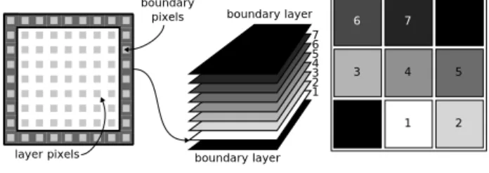
We used a collocated grid discretization to store our velocity, pressure and density data. These variables are defined at the center of the voxels of a grid. At each time step the content of these data sets should be refreshed. As we do all the simulation on the GPU, we should store this data on the graphics card's memory in a way that it can be efficiently read and written by the graphics processor. In GPU programming we usually store our data in textures. The problem with three dimensional data is that although the graphics cards support 3D data sets as 3D textures, no rendering is allowed to them. One can solve this problem with updating each slice of the volume into a separate texture and copy this data to the volume after refresh. This copy operation can take too much time making interactive rendering impossible for large data (this problem is solved by Shader Model 4 GPUs).

3 1 2 4 5 6 7

3D texture Flat 3D texture Slice layer pixels 1 2 3 4 boundary pixels _{6 7} 5 boundary layer boundary layer

Fig. 1. Volume slices and Flat 3D texture.

For efficiency reasons we used flat 3D textures as

described by Harris [5]. A flat 3D texture tiles the slices of a 3D volume into a 2D texture (see Fig.1.).

The result of the simulation is not only controlled by the external forces but also by the boundary conditions. These conditions describe what happens with the fluid at its boundary, i.e. on the faces of the cube encapsulating the grid volume. To store these conditions, we should extend each slice of the volume with one pixel border and we should also add two extra layers at the “top” and at the “bottom” of the volume.

Once the textures are ready, one simulation step of a layer of the volume can be done by the rendering of a quadrilateral, while boundary pixels are refreshed with rendering line primitives. As indexing a flat 3D texture needs extra work compared to usual 3D textures, we prepare a lookup texture which helps to index the origin of any layer in the flat 3D texture. The rendered quadrilaterals also store information about the location of the layers right above and below in the flat 3D texture.

Unlike in true 3D textures interpolating between two volume slices cannot be done by the texture units, thus interpolation is computed by custom shaders.

The simulation steps require to read and to write into a 3D data at the same time. Calculation one simulation step means rendering to a texture, but accessing a texture which is currently bound as a render target is not allowed. To overcome this limitation we should make a copy of our flat 3D textures - one will be sampled and one will be bound as a render target - and swap them after render (ping-ponging).

We used a 3D texture slicing rendering method to display the resulting display variable field, which means that we place semi-transparent polygons perpendicular to the view plane and blend them together in back to front order. The color and the opacity of the 3D texture is the function of the 3D display variable field.

Here we also had good use of the lookup texture to index our flat 3D textures to find the location of an arbitrary point in space in the tiled structure. Fig.4. shows one state of the flat 3D textures describing the velocity (right column) and display variable (left column) fields in a simulation. The top row shows these values with vorticity confinement turned off, and the bottom row shows the effect of vorticity confinement.

VII. SOLID OBSTACLES

If solid objects are present inside the fluid, the simulation should be modified. The density inside the voxels occupied by these objects should be zero, and the velocity should be set to the velocity of thee object [11]. Furthermore, the boundary conditions should be properly set at the solid-fluid boundary. The appropriate boundary condition is a free-slip condition, which states that fluid

velocity equals to the object velocity in the direction of the boundary normal. This prevents the fluid from entering the solid object, but can freely flow along its surface. The free slip condition can be enforced after pressure projection. We should correct the result of the projection step in the following way: if the boundary voxel along a direction is a solid object, then we should use the corresponding component of its velocity.

This requires the identification of voxels occupied by solid objects, and the determination of their velocity. In other words the object should be voxelized. To do this we create a separate grid containing the inside-outside information of the voxels and also the velocity values in the solid objects. We used an approach similar to [11], but we applied alpha blending instead of stencil operations. We render objects into each slice of the grid using an orthographic projection. The far clipping plane is set at infinity and the near clipping plane at the depth of the current slice. We render the object twice, once with back facing polygons and once with front facing polygons. We set up for additive blending and use value 1 for back faces and -1 for front faces. If the object is a closed shell, the result will contain a value 1 if the voxel is inside of the object and zero otherwise. If the mesh is a rigid mesh and does not deform, we can also write its velocity information into the first three components of this texture, while the alpha component stores the inside-outside information. In case of deformable objects like skinned characters special handling of the exact boundary is [11].

After voxelization the effect of solid object can be added to the velocity and density fields similarly to external forces.

VIII. DISTRIBUTED SYSTEM

Because of the data storing needs and computational cost described so far one can easily run into a point where a single computer implementation becomes insufficient. Using flat 3D textures has a disadvantage that they limit the size of the grid that can be simulated, as there is a limited texture size. Tiling the grid slices can easily result in a flat 3D texture with too high resolutions. The maximum resolution of the grid that can be computed is 254×254×254. We should note here that this grid resolution requires 4096×4096 flat 3D texture resolution since we need two extra slices and one extra pixel border in each slice for the boundary conditions.

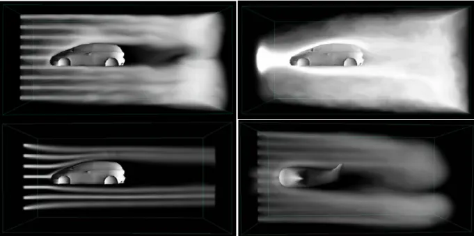
Fig. 2. Volume rendered with our distributed rendering algorithm. The wire cubes show one part of the grid which is

simulated on one node of the cluster.

One can step over this limit by subdividing the grid into smaller parts and store them in separate flat 3D textures, but can still run out of the GPU memory. On the other hand, the high computational cost of simulating high resolution grids does not allow interactive frame rates. The solution of these problems is the application of distributed GPGPU simulation and rendering.

We implemented our algorithm on a GPU cluster. This is a shared memory parallel rendering and compositing environment that uses the ParaComp library

(http://sourceforge.net/projects/paracomp) of the HP Scalable Visualization Array. The main aspect of this

library is that each host contributes to the pixels of rectangular image areas, called framelets. The process of

merging the pixels of framelets into a single image is called compositing. The ParaComp library allows not only

the framelet computation but also the composition to run parallely on the cluster. In our implementation one node takes the role of the master, which means that it has additional tasks beside rendering and compositing. The master sets the proper order of the nodes for composition and displays the composited image on screen. All nodes (including the master) do simulation steps on one portion of the data set, render the subvolume, and contributes this

image as one framelet. The composition of framelets is done with alpha blending in a parallel way using the

parallel pipeline algorithm [10].

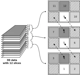
We used object space distribution of the 3D data (see Fig.3). We subdivided the grid and each part was treated as a separate data set. Each node in the distributed system should send the adjacent grid slices to its neighbors as a boundary condition to be used.

In Fig.3 the dashed arrows show the communication between the nodes in case of a three node system. For example, the topmost node sends its lowest layer to its lower neighbor, which puts this data to its topmost boundary condition layer. This neighboring node also sends its topmost slice to its upper neighbor, which puts this data in its lowest boundary condition slice. Three data should be transferred: the adjacent slices of the velocity, divergence variable s, and the display variable fields. We used an MPI implementation for boundary layer communication between nodes.

3 1 2 4 5 6 7 3D data

with 12 slices Node 1

10 8 9 11 12 9 10 11 12 5 6 7 8 1 2 3 4 Node 2 Node 3

Fig. 3. Data communication between the nodes of the cluster.

As we used a slicing rendering method to display the volume we should only ensure that the images produced by each node are composited in back to front order with alpha blending.

IX. RESULTS

For our experiments we used a Hewlett-Packard's Scalable Visualization Array consisting of five computing nodes.

Each node has a dual-core AMD Opteron 246 processor, an nVidia Quadro FX3450 graphics controller, and an InfiniBand network adapter. One node is only responsible for compositing and managing the framelet generations and does not take part in the rendering processes, so we could divide our data set into maximum four parts.

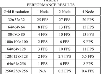
Table I. shows the performance results of the simulation of Figures 4 and 6. It can be seen that using 2 nodes gives better performance than the single computer version. Using more than 2 nodes becomes useful only in case of larger data sets, for small data sets the communication between the nodes becomes a bottleneck. The N/A sign means that a 256×256×256 data set cannot be simulated on a single computer since it has too high memory needs. It is worth examining the resolutions of 64×64×64 and 80×80×80. The 80 resolution needs about twice as many voxels as the 64 one. It can be clearly seen that the

performance of the two node implementation is the double of the performance obtained on a single computer. Similarly the two node implementation nearly doubles performance in almost all cases.

X. CONCLUSIONS

This paper showed that the computation of fluid simulation on a Cartesian grid can be effectively shared between nodes of a GPU cluster. Distributed simulation and rendering of fluid phenomena are necessary if the grid volume has higher resolution than the resolution a single GPU can cope with. Our implementation shows good scalability, and the simulation results do not suffer from visual artifacts.

TABLE I

PERFORMANCE RESULTS

Grid Resolution 1 Node 2 Node 4 Node 32×32×32 25 FPS 27 FPS 20 FPS 64×64×64 8 FPS 13 FPS 15 FPS 80×80×80 4 FPS 10 FPS 13 FPS 100×100×100 2 FPS 6 FPS 9 FPS 64×64×128 3 FPS 10 FPS 11 FPS 128×128×128 2 FPS 2.7 FPS 5.5 FPS 64×64×256 1 FPS 6 FPS 8 FPS 256×256×256 N/A 0.2 FPS 0.4 FPS ACKNOWLEDGEMENTS

This work has been supported by the National Office for Research and Technology (Hungary), Hewlett-Packard, by OTKA K-719922, and by the Croatian-Hungarian Action Fund CRO-35/2006.

REFERENCES

[1] Zhe Fan, Feng Qiu, Arie Kaufman, and Suzanne Yoakum-Stover, GPU cluster for high performance computing,

ACM/IEEE Supercomputing Conference, 2004.

[2] R. Fedkiw, J. Stam, and H. W. Jensen, Visual simulation of smoke, ACM SIGGRAPH 2001, pages 15–22, 2001.

[3] Nick Foster and Dimitris Metaxas, Modeling the motion of a hot, turbulent gas, Computer Graphics, 31(Annual

Conference Series):181–188, 1997.

[4] Mark Harris, Fast fluid dynamics simulation on the GPU,

SIGGRAPH ’05: ACM SIGGRAPH 2005 Courses, page 220, New York, NY, USA, 2005. ACM Press.

[5] M. Harris, W. Baxter, T. Scheuermann, and A. Lastra,

Simulation of cloud dynamics on graphics hardware,

Eurographics Graphics Hardware’2003, 2003.

[6] J. Krüger and R. Westermann, GPU simulation and rendering of volumetric effects for computer games and virtual environments, Computer Graphics Forum,

24(3):685–693, 2005.

[7] Natalya Tatarchuk Pedro V. Sander and Jason L. Mitchell,

Early-z culling for efficient GPU-based fluid simulation, in

Wolfgang Engel, editor, ShaderX5: Advanced Rendering Techniques, chapter 9.6, page 553-564. Charles River Media, Cambridge, MA, 2006.

[8] W. T. Reeves, Particle systems - techniques for modeling a class of fuzzy objects, SIGGRAPH ’83 Proceedings, pages

359–376, 1983.

[9] Jos Stam, Stable fluids, Proceedings of SIGGRAPH 99,

Computer Graphics Proceedings, Annual Conference Series, pages 121–128, August 1999.

[10] T.-Y. Lee, C. Raghavendra, and J. B. Nicholas, Image composition schemes for sort-last polygon rendering on 2D mesh multicomputers, IEEE Transactions on Visualization and Computer Graphics, 2 (1996).

[11] Keenan Crane, Ignacio Llamas, Sarah Tariq. Real-Time Simulation and Rendering of 3D Fluids. GPU Gems 3, Edited by Hubert Nguyen, Addison-Wesley 2007. pp.633-675.

Fig. 5. Interactive fluid simulation. Emitters are controlled by the cursor.

Fig. 6. Flat 3D velocity (upper row) and density (bottom row) textures of a simulation shown by Figure 4. The right column shows the simulation with vorticity confinement.