Universal Kriging of functional data:
trace-variography vs cross-variography?
Application to gas forecasting in unconventional shales
Alessandra Menafoglioa, Ognjen Grujicb, Jef Caersb
aMOX, Department of Mathematics, Politecnico di Milano bSchool of Earth, Energy & Environmental Sciences, Stanford University
Abstract
In this paper we investigate the practical and methodological use of Univer-sal Kriging of functional data to predict unconventional shale gas production in undrilled locations from known production data. In Universal Kriging of functional data, two approaches are considered: 1) estimation by means of Cok-riging of functional components (Universal CokCok-riging, UCok), requiring cross-variography and 2) estimation by means of trace-cross-variography (Universal Trace-Kriging, UTrK), which avoids cross-variogram modeling. While theoretically, under known variogram structures, such approaches may be quite equivalent, their practical application implies different estimation procedures and model-ing efforts. We investigate these differences from the methodological viewpoint and by means of a real field application in the Barnett shale play. An exten-sive Monte Carlo study inspired from such real field application is employed to support our conclusions.
Keywords: Geostatistics, functional data, trace-variogram, shale gas,
unconventional resources
1. Introduction
Functional data analysis (FDA, Ramsay and Silverman, 2005) has gained renewed attention in the modeling of phenomenon that can be regarded as sta-tistical observations displaying systematic variation. In particular in terms of time series, FDA has been considered as an alternative to multivariate analysis, where in FDA the data is seen as a single functional object with an underlying smooth dynamic that drives variation in time. While first applications have been in bio-informatics (see Ullah and Finch, 2013, for a recent review), FDA has been gaining attention both in the development of theory and in its appli-cation in the Earth & Environmental Sciences, for example in climate science (Besse et al., 2000), water resources (Josset et al., 2015; Satija and Caers, 2015), environmental science (Henderson, 2006; Yan et al., 2015; Sancho et al., 2015), oceanography (Nerini et al., 2010), land use (Besse et al., 2005) and geology (Mant´e and Stora, 2012; Menafoglio et al., 2014, 2015).
Particular to the application in the Earth Sciences is the spatial context and the need for spatial models for functional data, as has historically been developed in geostatistics (Matheron, 1969; Cressie, 1993). A recent body of theoretical work has been published, extending Ordinary Kriging to the func-tional case (e.g., Delicado et al., 2010; Nerini et al., 2010; Menafoglio et al., 2014; Menafoglio and Petris, 2015, and references therein). However, in sev-eral practical applications, there is a need to address phenomena that require non-stationary approaches in space. To address such need, Universal Kriging of spatial functional data has been proposed by Caballero et al. (2013); Menafoglio et al. (2013). An alternative approach to deal with non-stationarity is proposed by Ignaccolo et al. (2014).
In this work, we present a timely and economically important application of functional data, namely to the modeling and forecasting in unconventional shale resources. The term “unconventional” emanates from the way such resources are exploited: a sand-water mixture is injected into horizontal wells, fracturing nearly impermeable shale formations enabling production of commercially sig-nificant hydrocarbon volumes. Shale production can be considered as one of the driving factors for low oil/gas prices in 2015 (Mˇanescu and Nu˜no, 2015) which has put financial pressures on further resource development (“The Shale Indus-try Could Be Swallowed By Its Own Debt”, Bloomberg news, July 18, 2015). As a consequence, technical innovation is required for such resources to remain competitive with conventional exploitation which tend to have lower costs. In addition, better modeling, understanding and more optimal drilling practices will lead to lesser environmental impact (see, e.g., Vidic et al., 2013). Part of such technical innovation lies in understanding the impact of the geological and hydraulic fracturing factors on production, which drives the spatial variability of production in wells. Due to the complexity involved, statistical approaches based on data are preferred over physical modeling approaches (Mohaghegh, 2011, 2013; Kormaksson et al., 2015; Grujic et al., 2015). Production rates in wells start from an initial peak in production right after hydraulic fracturing followed by a long multi-month decline. In this paper, we focus on modeling the spatial distribution of production decline rates only. The latter are com-monly observed at discrete time points, at which the actual data are affected by a measurement error. In this case, a data preprocessing is required to obtain a set of smooth production rate curves from raw observations. This situation is quite common in FDA, and several smoothing methods are available in the literature, such as projection over a functional basis (e.g., Fourier, B-splines) or local polynomial smoothing (Ramsay and Silverman, 2005).
In this context, the first aim of this paper is to investigate the use of Univer-sal Kriging of functional data to the spatial interpolation of gas production rate curves (GPRCs) which is required to estimate production for undrilled location. Here, we consider data from the prolific Barnett Shale and our data set contains 922 wells drilled over the basin. Such dataset consists of functional data (de-cline rate) varying over space (geographic coordinates). Our second aim is to compare two approaches to the problem of functional Kriging: 1) estimation by means of Cokriging of the components over a functional basis (Universal
Cok-riging, UCok) which requires cross-variography, and 2) estimation by means of trace-variography (Universal Trace-Kriging, UTrK), which follows the approach of Menafoglio et al. (2013) and avoids cross-variogram modeling. The former constitutes an original extension to the non-stationary setting of the strategy of Nerini et al. (2010). Here, we show how to adapt the approach when rely-ing upon a functional principal component analysis, that allows to obtain an optimal and low dimensional basis representation of the observations. Our com-parison is with respect to the Barnett shale data set and a Monte Carlo study based on that dataset.
The paper structure is as follow. We first describe, in Section 2, the methods as well as provide an overview of the theoretical and methodological implications for comparison. Then in Section 3 we apply and evaluate both methods to the Barnett shale and provide and in-depth Monte Carlo comparison.
2. Methodology
In this Section, we pursue the functional and geostatistical approach to the analysis of GPRCs, and explore two alternative methods for their spatial pre-diction.
We call (Ω,F,P) a probability space, Ω denoting a space of events, F a σ
-algebra, andPa probability measure. We indicate by xs1, ..., xsn the observed
GPRCs1(possibly smoothed) at a set of given locationss
1, ...,snin an Euclidean spatial domainD⊆R2. As in classical geostatistics, we assume the data to be
a partial observation of a random field
{Xs,s∈D}, (1)
on (Ω,F,P), where the indexsindicates a location inD. As the observations are curves, the random field (1) is assumed to be valued in an infinite-dimensional (functional) space. Specifically, throughout this work we assume that, for any location s ∈ D, the element Xs is a random element of the space L2(T) of squared-integrable real-valued functions on the time intervalT = [1,60]. The spaceL2(T) (orL2 for short) is a separable Hilbert space if equipped with the
usual inner producthf, gi=R
Tf(t)g(t)dtand the induced normkfk=
p
hf, fi, forf, g∈L2(T).
We assume that process (1) is non-stationary, and represent its elementXs, at a generic location s ∈ D, as the sum of its mean ms, called drift, and a zero-mean stochastic residualδs that is stationary in the sense that is specified below, i.e.,
Xs=ms+δs. (2)
Here, the meanms of Xs can be defined point-wise as ms(·) = E[Xs(·)], and is a non-random element ofL2(T). Hereafter in this work, we assume that the
1To preserve the positivity of GPRCs, the model and the subsequent procedures can be
mean is non-constant in space, and we model its spatial variation through a functional linear model inL2(T) of the form
ms(t) = L
X
l=0
al(t)fl(s), t∈T,s∈D, (3)
where{al, l = 0, ..., L} are functional coefficients inL2(T), independent of the spatial location, while{fl(s), l= 0, ..., L}are known scalar regressors depending on s ∈ D. Finally, we assume that the residuals form a zero-mean random field{δs,s∈D} on (Ω,F,P), with stationary spatial covariance function. The
latter is defined as the function that maps any increment between locations in D, (s1−s2) ∈ R2, into the cross-covariance operator on L2(T) between the
elements of the process at those locations:
C(s1−s2)x=E[hδs1, xiδs2], x∈L
2(T). (4)
Under these assumptions, and given the random observationsXs1, ..., Xsnat
the sampled locations, we aim to predict the unobserved elementXs0 of process
(1) at a target locations0∈D.
2.1. Universal Cokriging of functional data
We here present a novel and original extension to the non-stationary setting of the Kriging predictor for functional data proposed by Giraldo (2009) and Nerini et al. (2010).
Throughout this Subsection, we consider an orthonormal set {ek,1 ≤ k ≤ K}inL2(T), and we assume that each element of process (1) can be represented
through the expansion over this set, i.e.,
Xs= K
X
k=1
ξk(s)ek, s∈D, (5)
whereξk(s) =hXs, ekiis the projection ofXson thek-th element of the basis. Under representation (5), one can characterize process (1) through the distri-butional properties of theK-dimensional random field of coefficients{ξ(s),s∈
D}, with ξ(s) = (ξ1(s), ..., ξK(s))T. For instance, one can define the drift ms of the process atsinD, through the drift of the field{ξ(s),s∈D}at the same location,mξ(s) = (mξ 1(s), ..., m ξ K(s)) T, ms(·) = K X k=1 E[ξk(s)]ek(·) = K X k=1 mξk(s)ek(·). (6)
Note that under model (3), the drift of the coefficients field is described by the linear model mξk(s) = L X l=0 αklfl(s), s∈D, (7)
withαkl =hal, eki. Indeed, one has hms, eki= L X l=0 hal, ekifl(s) =m ξ k(s), (8)
where the first equality follows from Eq. (3), and the second equality is obtained by using Eq. (6). We thus represent the elements of the multivariate field
{ξ(s),s∈D} as
ξ(s) =mξ(s) +(s), (9)
where{(s),s∈D}forms a zero-meanK-dimensional random field. If the assumption of second-order stationarity (in L2(T)) for {δ
s,s ∈ D}
holds true, then also{(s),s∈D}is second-order stationary (inRK). Indeed,
under representation (5), one has the following matrix representation of the spatial covariance functionC
C(s1−s2)x= K X j=1 K X k=1 Cjkξ (s1−s2)xjek, s1,s2∈D, (10)
where Cjkξ (s1−s2) = hC(s1−s2)ej, eki. The latter quantity is equivalently found as the covariance between the coefficientsξj(s1) andξk(s2):
Cjkξ(s1−s2) =E[(ξj(s1)−m
ξ
j(s1))(ξk(s2)−m
ξ
k(s2))]. (11)
As such, the cross-covariogram ofξj andξk is stationary for allj, k= 1, ..., K. Given the observations Xs1, ..., Xsn, we aim to predict Xs0 via the Best
Linear Unbiased Predictor (BLUP) in the sense of Nerini et al. (2010), that is Xs∗ 0 = Pn i=1Λ ∗ iXsi, where Λ ∗
1, ...,Λ∗nare the operators that solve the constrained optimization problem min E Xs0− n X i=1 ΛiXsi 2 s.t. E " Xs0− n X i=1 ΛiXsi # = 0, (12)
among all the linear Hilbert-Schmidt operators Λ1, ...,Λn on L2(T). We call
Universal Cokriging (UCok) predictor the solutionX∗
s0 of problem (12).
Finding the UCok predictor is equivalent to determine an optimal estimate of the coefficients vectorξ(s0) at the target locations0by solving the following
Cokriging problem min E ξ(s0)− n X i=1 Liξ(si) 2 RK s.t. E " ξ(s0)− n X i=1 Liξ(si) # =0, (13)
among all the matrices of weightsL1, ...,Ln inRK×K. Similar to the stationary
setting (Nerini et al., 2010), this follows from the observation that (i) the op-erators Λi, i= 1, ..., n, admit a matrix representation through Li, i= 1, ..., n,
analogous to that ofCin Eq. (10); (ii) by exploiting expression (5) and Parsival identity, one has that the objective functionals in Eqs. (12) and (13) coincide; and (iii) by developing the unbiasedness constraint in Eq. (12) in the light of Eq. (5) one gets
E " Xs0− n X i=1 ΛiXsi # = K X k=1 E " ξk(s0)− " n X i=1 Liξ(si) # k # ek, (14)
which is the null function if and only if E[ξ(s0)−P
n
i=1Liξ(si)] is the null vector inRK.
Therefore, the UCok predictorXs∗0ofXs0can be found asX
∗ s0 = PK k=1ξk∗(s0)ek, whereξ∗(s0) =P n
i=1L∗iξ(si) and the optimal matrices of weights are found by solving the Universal Cokriging system (Chil`es and Delfiner, 1999)
C11 · · · C1n F10 · · · F1L .. . . .. ... ... . .. ... Cn1 · · · Cnn Fn0 · · · FnL F10 · · · Fn0 0 · · · 0 .. . . .. ... ... . .. ... F1L · · · FnL 0 · · · 0 L1 .. . Ln Z0 .. . ZL = C01 .. . C0n F00 .. . F0L , (15)
whereCij is the cross-covariance matrix betweenξ(si) andξ(sj),i, j= 1, ..., n;
Ci0 is the cross-covariance matrix between ξ(s0) andξ(si), i = 1, ..., n; Fil = diag(fl(si), ..., fl(si))∈RK×K andZl,l= 0, ..., Lare the matrices of Lagrange
multipliers.
2.2. Universal Trace-Kriging
In this Subsection, we recall an alternative approach to Kriging, which has been proposed by Menafoglio et al. (2013). Such approach enables one to get rid of the assumption of the basis representation (5) by defining a different measure of spatial dependence.
Call trace-covariogram of the residual field{δs,s∈D}, the real-valued func-tionCtr defined, fors1,s2 inD and in the previous assumptions, as
Ctr(s1−s2) =E[hδs1, δs2i]. (16)
The trace-covariogram defines a global measure of spatial dependence, in the sense that, for any fixed increment (s1−s2) inR2, it is the trace of the
corre-sponding cross-covariance operatorC(s1−s2). The trace-covariogram plays the
same role as the univariate covariogram, but in the infinite-dimensional setting. Here, the corresponding trace-variogram is defined as
2γtr(s1−s2) =E[kδs1−δs2k
2], (17)
and describes the expected increment in the value of the (functional) process for a given increment in the spatial domain. On these bases, Menafoglio et al.
(2013) define and explore a global notion of stationarity for functional random fields, weaker than that considered so far. For sake of clarity in the following comparisons, we here keep the same stationarity assumption on the residual field as those introduced before.
To predict the unobserved elementXs0, given the observationsXs1, ..., Xsn,
Menafoglio et al. (2013) consider a Kriging predictor in the form of a linear com-bination of the observations. We call Universal Trace-Kriging (UTrK) predictor the linear unbiased predictorX∗tr
s0 = Pn i=1λ ∗ iXsi, whose weightsλ ∗ 1, ..., λ∗n solve min E Xs0− n X i=1 λiXsi 2 s.t. E " Xs0− n X i=1 λiXsi # = 0, (18)
over all the scalar weightsλ1, ..., λninR. The authors then prove that problem
(18) is well-posed even if one relies only upon the global definitions of spa-tial dependence introduced above. Indeed, the weightsλ∗
1, ..., λ∗n are found by solving Ctr(0) · · · Ctr(h1n) f0(s1) · · · fL(s1) .. . . .. ... ... . .. ... Ctr(hn1) · · · Ctr(0) f0(sn) · · · fL(sn) f0(s1) · · · f0(sn) 0 · · · 0 .. . . .. ... ... . .. ... fL(s1) · · · fL(sn) 0 · · · 0 λ1 .. . λn ζ0 .. . ζL = Ctr(h10) .. . Ctr(hn0) f0(s0) .. . fL(s0) , (19) withhij =si−sj, and ζ0, ..., ζL the Lagrange multipliers associated with the (L+ 1) unbiasedness constraints.
2.3. Methodological comparison
Even though the methods devised in Subsections 2.1 and 2.2 do achieve the same purpose, namely the geostatistical prediction of functional data, they are intrinsically different. We here compare the different perspectives they are grounded on, to underline the methodological strengths and weaknesses of the two approaches to deal with real studies.
Data Representation. The derivation of the UCok predictor relies upon the assumption that the elements of the process admit expansion (5), for a given order K and an orthonormal set {ek,1 ≤ k ≤ K}. In FDA, this is a viable assumption, as analyses in this field commonly employ a preprocessing step (or smoothing) based on an expansion over a truncated functional basis (e.g., Fourier basis). This step enables one to smooth the actual discrete ob-servations, by removing from the measured curves the effects that are chiefly due to the measurement error. Non-orthonormal bases may be employed in the smoothing procedure (e.g., B-splines). Nevertheless, one can always perform a change of basis to map the observations on an orthonormal set, and accordingly
represent the process via expansion (5).
Data Dimensionality and Problem Complexity. Even though expan-sion (5) does not imply a substantial loss of generality in most real studies, the dimension of the expansion is influential indeed on the analysis. Indeed, as noted by Menafoglio and Petris (2015) in the stationary setting, even in the ideal case of known drift and covariance structure, the parameterK controls the dimen-sion of system (15) (i.e., the numberK(n+L+ 1) of equations and unknowns), hence the problem complexity. Thus, in a real case study, one may need to em-ploy a dimensionality reduction method prior to the geostatistical analysis. For instance, one can perform Functional Principal Component Analysis (FPCA, Ramsay and Silverman, 2005) as detailed in the Appendix, or the Functional Singular Value Decomposition (FSVD, Yang et al., 2011). In all these cases, part of the information is inevitably lost as a consequence of the dimensionality reduction, and cannot be employed for prediction purposes. This marks the first difference between Universal Cokriging and Universal Trace-Kriging methodolo-gies, as the latter does not require to express the observations through a basis representation and/or reduce their dimensionality. In fact, the dimensionality of the Trace-Kriging system does not depend on the representation of the data: system (19) is a linear system of (n+L+ 1) equations with the same number of unknowns, independently of the possible truncated basis expansion employed to represent the data. Notice that this is possible because of the simple form of the UTrK predictor, as opposed to the more complex form of the UCok pre-dictor. This is both a weakness and a strength of Trace-Kriging. On one hand, the UCok predictor is more general and, in principle, able to achieve a better prediction quality than the UTrK predictor. On the other hand, the simple form of the UTrK allows to exploit the entire information embedded into the data, without the need to reduce the dimensionality of the dataset prior to the geostatistical analysis.
Variogram Estimation. In the context of Gaussian stationary random fields and under the representation (5), with K ≤ n, a formal relation be-tween the Cokriging and the Trace-Kriging predictors has been established by Menafoglio and Petris (2015). In this framework, the authors prove that the Cokriging and Trace-Kriging approaches lead almost surely to the same results, provided that the spatial covariance functionCis known. In most applications, the spatial dependence is actually not knowna priori and one needs to inferC from available data (or basis coefficients). To this end, different viewpoints on the Kriging problem induce different ways to estimate the spatial covariance. If one is willing to solve the Universal Cokriging system (15), the covariograms and cross-covariogram of the coefficients will be the target estimates. To this end, a Linear Model of Coregionalization (LMC) can be introduced for the vec-tor of coefficients, and a parametric semivariogram structure can be fitted to the empirical estimates. Note that the dimension K of the representation (5) directly reflects on the number of variogram and cross-variogram structures that one needs to estimate to solve Eq. (15). In contrast, to solve system (19) one
will only estimate the trace-covariogram, or the trace-variogram as usually pre-ferred. Estimating the latter follows the same line as in finite dimension. First an empirical estimate is computed from (estimated) residuals as
γ(h) = 1 2|N(h)| X (i,j)∈N(h) kδsi−δsjk 2, (20)
wherehdenotes the lag,N(h) the set of couples at laghand|N(h)|the num-ber of elements of setN(h). Second, a valid variogram model is fitted to the empirical estimate. Here, the well-known one-dimensional parametric families, such as spherical or Mat´ern, can be employed. Note that estimator (20) requires to compute a number of integrals (recall:kf−gk2=R
T(f(t)−g(t)
2dt, forf, gin
L2(T)). These can be computed in terms of basis coefficients whenever a basis
representation of the kind (5) is employed, or via quadrature schemes otherwise.
Joint Estimation of the Parameters. To estimate the drift, the resid-uals and the variogram structure, one can employ very similar strategies in both the discussed approaches. In this work, we estimate the drift mξ via Generalized Least Squares (GLS), and employ the classical iterative algorithm to jointly estimate the drift via GLS and the variograms/cross-variograms of the corresponding residuals. Similarly, we estimate via GLS the drift ms, as follows (see Menafoglio et al., 2013). We call Σ the global covariance matrix Σij =E[hδsi, δsji],Fthe design matrix [F]il=fl(si),i= 1, ..., n,l= 0, ..., L,X
the vector of functional observationsX = (Xs1, ..., Xsn)
T ∈L2× · · · ×L2 and
we introduce the following matrix notation: [Af]i=Pnj=1Aijfj, forA∈Rn×n,
f ∈L2× · · · ×L2. The GLS estimator of the drift at the observed locations,
m= (ms1, ..., msn)
T, is (Menafoglio et al., 2013)
c
m=F(FTΣ−1F)−1FTΣ−1X. (21)
Similarly as in the classical setting, mc can be computed by resorting to an iterative algorithm: having initializedmc(e.g., to the ordinary least square es-timate obtained by setting Σ to a multiple of the identity matrix in Eq. (21)), at each step the residuals are estimated by difference from the GLS estimate of the drift, and then the trace-variogram is estimated from the latest update of the residuals estimate. We refer to Menafoglio et al. (2013) for the algorithmic details.
In the next Section we compare the results of applying these different strate-gies to the dataset of GPRCs available at the Barnett Shale field site.
3. An Application: Analysis of Gas Production Rate Curves in the Barnett Shale
3.1. Dataset Description
In this study we use gas production rate curves (GPRC) from 922 wells drilled in the Barnett shale, one of the most prolific and the most developed
unconventional gas reservoirs in North America. This dataset was compiled from the “drillinginfo.com” (further DI), an online oil and gas data repository. Amongst the data available on DI, the 922 wells used for the present analysis were selected according to the following criteria. At the time when this dataset was prepared, DI did not provide information about well specific hydraulic frac-turing parameters, which would have enabled us to search for wells with similar completions. Therefore, we decided to query for wells whose lateral length was anywhere between 1800 and 2300 feet and were owned by the same company (operator), with an assumption that the number of hydraulic fractures was the same or at least very similar across all wells. We considered wells drilled after 2005, which had at least 5 years of production history (60 months), immediately following the peak gas rate. As a part of pre-processing, all data entries preced-ing the peak gas rates (about 3 months) were discarded. Such pre-processpreced-ing approach is very common in unconventional reservoir data analyses (see Patzek et al., 2013), since during that time period wells mostly produce flow-back water that comes as a consequence of hydraulic fracturing.
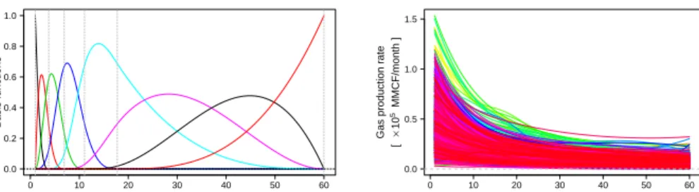
As a first step of the analysis we performed a data smoothing to obtain smooth curves from raw observations. In ideal conditions2, GPRCs are smooth and monotonically decreasing positive curves. In such setting there is a complete absence of periodicity and B-Spline basis system comes as a natural choice for representing the data. To honor the data positivity, we elected to perform basis expansion on the log-transformed observations, with a smoothing penalty on the second derivative. Preliminary data analysis revealed that most variation in GPRCs occurred during the first 12 months of production history. Therefore, we decided to place the knots of B-spline basis functions irregularly over analyzed time domain (60 months), with higher placement density over the first 12 months (Figure 1 Left). Finally, the number of basis functions for this dataset was set to n= 10, and the best smoothing penalty on the second derivative (λ= 103) was
found with generalized cross validation (GCV, Ramsay and Silverman, 2005). Figure 1 shows final B-spline basis system (left) with resulting smoothed GPRCs (right).
3.2. Results
We first analyzed the smoothed dataset according to the approach devised in Subsection 2.2. For the analyses that follow we considered the log-transformed GPRCs (further log-GPRCs) to honor the positivity constraint. Hereafter we display the results in the original scale to ease their interpretation.
Based on preliminary analyses at the site, we selected for the drift term the set of linear regressors in the spatial coordinates:f0(s) = 1;f1(s) =x;f2(s) =y,
s= (x, y) denoting a location inD. Following the strategy detailed in Subsec-tion 2.3, we jointly estimate the drift and the trace-variogram, fitting to the lat-ter a spherical model with nugget. Figure 2 shows the empirical trace-variogram along with the fitted model.
0 10 20 30 40 50 60 0.0 0.2 0.4 0.6 0.8 1.0 time [month] Basis functions 0 10 20 30 40 50 60 0.0 0.5 1.0 1.5 time [month] Gas production r ate [ × 10 5 MMCF/month ]
Figure 1: Left: final basis system found by the GCV on GPRCs; Right: Smoothed GPRCs. Gas rates are given in MMCF per month.
● ● ● ● ● ● ● ● 0 500 1500 2500 0 5 10 15 20 Distance [km] T race−semiv ar iogr am 3459 1830332411 41341 47521492714917445389
Figure 2: Estimated trace-variogram of log-GPRCs at the Barnett shale: empirical estimate (symbols), calibrated model (solid line). Numbers indicate the number of couples of locations upon which the corresponding empirical estimate is based.
0 10 20 30 40 50 60 0.0 0.5 1.0 1.5 time [month] Gas production r ate [ × 10 5 MMCF/month ] ● ● ● ● ● ● ● ● ● ● ● ● ● ● ● ● ● ● ● ● ● ● ● ● ●●● ● ● ● ● ● ● ● ● ● ● ● ● ● ● ● ● ● ● ● ● ● ● ● ● ● ● ● ● ● ● ● ● ● ● ● ● ● ● ● ● ● ● ● ● ● ● ●● ● ● ● ● ● ● ● ● ● ● ● ● ● ● ● ● ● ● ● ● ● ● ● ● ● ● ● ● ● ● ● ● ● ● ● ● ● ● ● ● ● ● ● ● ● ● ● ● ● ● ● ● ● ● ● ● ● ● ● ● ● ● ● ● ● ● ● ● ● ● ● ● ● ● ● ● ● ● ● ● ● ● ● ● ● ● ● ● ● ● ● ● ● ● ● ● ● ● ● ● ● ● ● ● ● ● ● ● ● ● ● ● ● ● ● ● ● ● ● ● ● ● ● ● ● ● ● ● ● ● ● ● ● ● ● ● ● ● ● ● ● ● ● ● ● ● ● ● ● ● ● ● ● ● ● ● ● ● ● ● ● ● ● ● ● ● ● ● ● ● ● ●● ● ● ● ● ● ● ● ● ● ● ● ● ● ● ● ●● ● ● ● ● ● ● ● ● ● ● ● ● ● ● ● ● ● ● ● ● ● ● ● ● ● ● ● ● ● ● ● ● ● ● ● ●● ● ● ● ● ● ● ● ● ●● ● ● ● ● ● ● ● ● ● ● ● ● ● ● ● ● ● ● ● ● ● ● ● ● ● ● ● ● ● ● ● ● ● ● ● ● ● ● ● ● ● ● ● ● ● ● ● ● ● ● ● ● ● ● ● ● ● ● ● ● ● ● ● ● ●● ● ● ●● ● ● ● ● ● ● ● ● ● ● ● ● ● ● ●● ● ● ● ● ● ● ● ● ● ● ● ● ● ● ● ● ● ● ● ● ● ● ● ● ● ● ● ● ● ● ● ● ● ●● ● ● ● ● ● ● ● ● ● ● ● ● ● ● ● ●●● ● ● ● ● ● ● ● ● ●● ● ● ● ● ● ● ● ● ● ● ● ● ● ● ● ● ● ● ● ● ● ● ● ● ● ● ● ● ● ● ● ● ● ● ● ● ● ● ● ● ● ● ● ● ● ● ● ● ● ● ● ● ● ● ● ● ● ● ● ● ● ● ● ●● ● ● ● ● ● ● ●● ● ● ● ● ● ● ● ● ● ● ● ● ● ● ● ● ● ● ● ● ● ● ● ● ● ● ● ● ● ● ● ● ● ● ● ● ● ● ● ● ● ● ● ● ● ● ● ● ● ● ● ● ● ● ● ● ● ● ● ● ● ● ● ● ● ● ● ● ● ● ● ● ● ● ● ● ● ● ●● ● ● ● ● ● ● ● ● ● ● ● ● ●● ● ● ● ● ● ● ● ● ● ● ● ● ● ● ● ● ● ● ● ● ●● ● ● ● ● ● ● ● ● ● ● ● ● ● ● ● ● ● ● ● ● ● ● ● ● ● ● ● ● ● ● ● ● ● ● ● ● ● ● ● ● ● ● ● ● ● ●● ● ● ● ● ●●● ● ● ● ● ● ● ● ● ● ● ● ● ● ● ● ● ● ● ● ● ● ● ● ● ● ● ● ● ● ● ● ● ● ● ● ● ● ● ● ● ● ● ● ● ● ● ● ● ● ● ● ● ● ● ● ● ● ● ● ● ● ● ● ● ● ● ● ● ● ● ● ● ● ● ● ● ● ● ● ● ● ● ● ● ● ● ● ● ● ● ● ● ● ● ●● ● ● ● ● ● ● ● ● ● ● ● ● ● ● ● ● ● ● ● ● ● ● ● ● ● ● ● ● ● ● ● ● ● ● ● ● ● ● ● ● ● ● ● ● ● ● ● ● ● ● ● ● ● ● ● ● ●● ● ● ●● ● ● ● ● ● ● ● ● ● ● ● ● ● ● ●● ● ● ●● ● ● ● ● ● ● ● ● ● ● ● ● ● ● ● ● ● ● ● ● ● ● ● ● ● ● ● ● ● ● ● ● ● ● ● ● ● ●●● 630000 650000 670000 3560000 3580000 3600000 3620000 X Y ●● ● ● ● ● ● ● ● ● ● ● ● ● ●● ● ● ● ●
Figure 3: Prediction by UTrK of GPRCs for 20 random locations at the Barnett shale. Left: smoothed data (grey lines) and predictions (colored lines). Right: sampled location (grey symbols) and target locations (colored symbol).
0.2 0.3 0.3 0.3 0.4 0.4 0.4 0.4 0.5 0.5 0.6 0.6 0.7 0.7 t = 1 month 0.1 0.15 0.2 0.2 0.2 0.2 0.25 0.25 0.25 0.3 0.35 t = 12 months 0.1 0.1 0.15 0.15 0.15 0.2 0.2 0.2 t = 24 months 0.04 0.04 0.06 0.08 0.08 0.08 0.1 0.1 0.1 0.12 0.12 t = 48 months
Figure 4: Prediction maps obtained with UTrK at the Barnett shale, fort = 1,12,24,48 months. Colors are given on a non-uniform scale. Gas rate reported on contour lines are meant up to a factor 105.
Based on the calibrated trace-variogram model, we performed a UTrK pre-diction over a uniform spatial grid of 104 locations at the field site. Figure 3
reports a subsample of 20 predicted GPRCs, for a randomly selected set of 20 location of the prediction grid. Graphical inspection of Figure 3 highlights that UTrK predictions are affected by a smoothing effect, amplified by the small size of the selected sample. In general, a similar smoothing effect is well-documented in the geostatistical literature on classical Kriging. Accordingly, extremes tend to be smoothed, especially when curves at nearby locations are not representa-tive of the same extreme behavior. A better reproduction of extreme behavior may be attained in the presence of covariates (external drift) related to geolog-ical/production variables.
Figure 4 reports the maps of the predicted functional field, taken for the time instantst = 1,12,24,48 months (colors are given on a non-uniform color scale). Note that, unlike multivariate techniques, a functional prediction allows to obtain simultaneous Kriging maps for any instant pointt∈[1,60] (months). To compare these predictions with those obtained through UCok, we
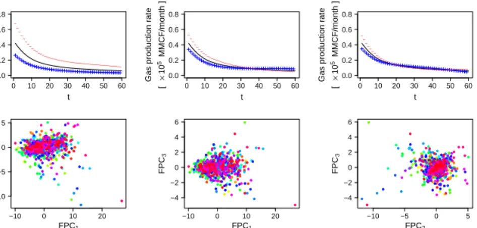
per-0 10 20 30 40 50 60 0.0 0.2 0.4 0.6 0.8 FPC1(82% of the variability) t Gas production r ate [ × 10 5 MMCF/month ] − − − − − −− −− −−− −−−−−−−−−−−−−−−− −−−−−−−−−−−−−−−−−−−−−− 0 10 20 30 40 50 60 0.0 0.2 0.4 0.6 0.8 FPC2(12% of the variability) t Gas production r ate [ × 10 5 MMCF/month ] − − − −− −− −−− −−−−−−−−−−−−− −−−−−−−−−−−−−−−−−−−−−−−−−−− 0 10 20 30 40 50 60 0.0 0.2 0.4 0.6 0.8 FPC3(4% of the variability) t Gas production r ate [ × 10 5 MMCF/month ] − − − − − −− −− −−−−−−−−−−− −−−−−−−−−−−−−−−−−−−−−−−−−−−−−− ● ● ● ● ● ● ● ● ●● ● ● ● ● ● ● ● ● ●●●● ● ● ● ●● ● ● ● ● ● ● ●● ● ●● ● ● ● ● ● ● ● ● ●● ● ● ● ● ● ● ● ● ● ● ● ● ● ● ● ● ●● ● ● ● ● ● ● ● ● ● ● ● ●●●● ● ● ● ● ● ● ● ● ● ● ● ● ● ● ● ● ● ● ● ● ●● ● ● ●● ● ● ● ● ● ● ● ● ● ● ● ● ●● ● ● ● ● ● ● ● ● ● ● ● ● ● ● ● ● ● ● ● ● ● ● ● ● ● ● ● ●● ● ● ● ● ● ● ● ● ● ● ● ● ● ● ● ● ● ● ● ● ● ● ● ● ● ● ● ● ● ● ● ● ● ●● ● ● ●● ● ● ● ● ● ● ● ● ● ● ● ● ● ● ● ● ● ● ● ● ● ● ● ● ● ● ● ● ● ● ● ● ● ● ● ● ● ● ● ● ● ● ● ● ●●● ●● ● ● ● ● ● ● ● ● ● ● ● ● ● ● ● ● ● ● ● ● ● ● ● ● ● ● ● ● ● ● ● ● ● ● ● ● ● ● ● ● ● ● ● ● ● ● ● ● ● ● ● ● ● ● ● ● ● ● ● ●● ● ● ● ● ● ● ●● ● ● ● ● ● ● ● ● ● ● ● ● ● ● ●● ● ● ● ● ● ● ● ● ● ● ●● ● ● ● ● ● ● ● ● ● ● ● ● ● ● ●● ● ● ● ●●● ● ● ● ●● ● ● ● ● ● ● ● ● ● ● ● ●● ● ● ● ● ● ● ● ● ● ● ● ● ● ● ● ● ● ● ● ● ● ● ● ● ● ● ● ● ● ● ● ● ●● ● ● ● ● ● ● ●● ● ● ● ● ●● ● ● ● ● ● ● ● ● ● ● ● ● ● ● ● ● ● ●●● ● ● ● ● ● ● ● ● ● ● ● ● ● ● ● ● ● ● ● ● ● ● ● ● ●●● ● ● ● ●● ● ●●●● ● ● ● ● ● ● ● ● ●●● ● ● ● ● ● ● ● ● ● ● ● ●● ● ● ● ● ● ● ● ● ● ● ● ● ● ● ● ● ● ● ● ● ● ● ● ●●●● ● ● ● ● ● ● ● ● ● ● ●● ● ● ● ● ● ● ● ● ● ● ● ● ● ● ● ● ● ● ● ● ● ● ● ● ● ● ● ● ●● ● ● ● ● ● ● ● ● ●● ● ● ● ● ● ● ● ● ● ● ● ●● ● ● ● ● ● ● ● ● ●● ● ● ● ● ● ● ● ● ● ● ● ● ● ● ● ● ● ● ● ● ● ● ● ● ● ● ● ● ● ● ●● ● ● ● ● ● ● ● ● ● ● ● ● ● ● ● ● ● ● ● ●●● ● ● ●● ●● ●● ● ●●● ●● ● ● ● ● ● ● ●●● ● ● ● ● ● ● ● ● ● ● ● ● ● ●●● ● ● ● ● ● ● ● ● ● ● ● ● ●● ● ● ● ● ● ● ● ● ● ● ● ● ● ● ● ● ● ● ● ● ● ● ●●● ●● ● ● ● ● ● ● ● ● ● ● ● ●●●●●● ● ● ● ●● ● ● ● ● ● ● ● ● ● ● ● ● ● ● ● ● ●● ●●● ● ● ● ●●● ● ●●● ● ● ● ● ● ● ● ●● ● ● ●● ● ● ● ● ● ● ●●● ● ● ● ● ● ● ● ● ● ● ● ● ● ● ● ● ● ● ● ● ● ● ● ● ● ● ● ● ● ●● ● ● ● ● ● ● ● ● ● ● ● ● ● ● ● ● ● ● ● ● ● ● ● ● ● ● ● ● ● ● ● ● ● ● ●●● ●● ● ● ●● ● ● ● ● ● ● ● ● ●● ● ● ● ● ● ● ● ● ● ● ● ●● ● ● ● ● ● ● ● ●●● −10 0 10 20 −10 −5 0 5 FPC1 F P C2 ● ● ● ● ● ● ●● ● ● ●● ● ● ● ● ● ● ● ●● ● ● ● ● ● ● ● ● ● ● ●● ●● ● ● ● ● ● ● ● ● ● ● ● ● ● ● ● ● ● ● ●● ● ● ● ● ● ● ● ●● ●● ● ● ● ● ● ● ●● ● ● ●● ●● ● ● ● ● ● ● ●●● ● ● ● ● ● ● ● ● ● ● ● ● ● ● ● ● ● ●● ● ● ● ● ● ● ● ● ● ● ● ● ● ● ● ● ● ● ● ● ● ●● ●● ● ● ● ● ● ● ● ● ●● ● ● ● ● ● ● ● ● ● ● ● ● ● ● ● ● ● ● ● ●●● ● ● ● ● ●● ● ● ● ● ● ● ● ● ● ●● ● ● ● ● ● ●● ● ● ● ● ● ● ● ● ● ● ● ● ● ● ● ● ● ●●●●● ● ● ● ● ● ● ●● ● ● ● ● ● ● ● ● ● ● ●●● ● ●●● ● ● ● ● ● ● ● ● ● ● ● ●● ● ● ● ● ●● ● ● ● ● ● ● ● ● ● ● ● ● ● ● ● ● ● ● ● ● ● ● ● ● ● ● ● ● ● ● ● ● ● ● ● ● ● ● ● ● ● ● ● ● ● ● ● ● ● ● ● ● ● ● ● ● ● ● ● ● ● ● ● ● ● ● ● ● ● ● ● ● ● ●● ● ● ● ●● ● ● ●● ● ● ● ● ● ● ●● ● ● ● ● ● ● ● ● ● ● ● ● ● ● ● ● ● ● ● ● ● ● ● ● ● ● ●● ● ● ● ● ● ● ● ●●●●● ● ● ● ● ● ● ● ●● ● ● ●● ●●● ● ● ● ● ● ● ● ● ● ● ● ● ● ●●● ● ● ● ● ● ● ● ● ● ● ● ● ● ● ● ● ● ● ● ● ● ●●● ● ● ● ● ● ● ● ● ● ● ● ● ● ● ● ● ● ● ● ● ● ● ● ● ● ● ●● ● ● ● ● ● ●● ●● ● ● ● ● ●● ● ● ●● ● ● ● ● ● ● ● ● ● ● ● ● ●● ● ● ● ● ● ● ● ● ● ● ● ● ● ● ● ● ● ● ● ● ● ● ● ● ● ● ● ● ● ● ● ● ● ● ● ● ● ● ● ● ● ● ● ● ● ● ● ● ● ● ● ● ● ● ● ● ● ● ● ● ● ● ● ● ● ● ● ●● ● ● ● ● ● ● ● ● ● ● ● ● ● ● ● ●● ● ● ● ● ●● ● ● ● ● ● ● ● ● ● ● ● ● ● ● ● ● ● ● ●● ● ● ● ● ● ● ● ● ● ● ● ● ● ● ● ● ● ● ● ● ● ● ●● ● ● ● ● ● ● ● ● ● ● ● ● ● ● ● ● ● ● ● ● ● ● ● ● ● ● ● ● ● ● ● ● ● ● ● ● ●● ● ● ● ● ● ● ● ●● ● ● ● ● ● ● ● ● ● ● ● ● ● ● ●● ● ● ● ● ● ● ● ● ● ● ● ● ● ● ● ● ● ● ● ● ● ● ● ● ● ● ● ● ● ● ● ● ● ● ● ● ● ● ● ● ● ● ● ● ● ●● ● ●● ● ● ●● ● ● ● ● ● ● ● ● ● ● ● ● ● ●●●● ● ● ● ● ●● ●●● ● ● ● ●● ● ● ● ● ● ● ● ● ● ● ● ● ● ● ● ● ●● ● ● ● ● ● ● ● ● ● ● ● ● ● ●● ●● ● ● ● ● ●● ● ● ● ● ●● ● ● ● ● ●●● ● ● ● ● ● ● ● ● ● ● ● ● ● ● ● ● ● ● ● ● ● ● ● ● ● ● ● ● ● ● ● ● ● ● ● ● ● ● ● ● ● ● ● ● ● ● ● ●● ● ● ● ● ● ● ● ● ● ● ● ● ● ● ● ● ● ● ● ● ● ● ● ● ● ● ● ● ● ● ● −10 0 10 20 −4 −2 0 2 4 6 FPC1 F P C3 ● ●● ● ● ●● ●● ●●● ● ● ● ● ● ● ● ●● ●● ● ● ● ● ● ● ● ● ● ● ●● ● ●● ● ● ● ● ● ● ● ●● ● ● ● ● ● ● ● ● ● ● ● ● ● ● ● ● ● ●● ● ● ● ● ● ● ● ● ● ● ● ●●●● ● ● ● ● ● ● ● ● ● ● ● ● ● ● ● ● ● ● ● ● ● ● ● ● ● ●● ● ● ● ● ● ● ● ● ● ● ● ● ● ● ● ● ● ● ● ● ● ● ● ● ● ● ● ● ● ● ● ● ● ●● ● ● ● ● ●● ● ● ● ● ● ● ● ● ● ● ●● ●●●●● ● ●● ●● ● ● ● ● ● ● ● ● ● ● ●●● ● ● ● ●● ● ● ● ● ● ● ● ● ● ● ● ● ● ● ● ● ● ● ● ● ●● ● ● ● ● ● ● ● ● ● ● ● ● ● ● ● ● ● ● ● ● ● ● ●●● ● ● ● ● ● ● ● ●●● ● ● ● ● ● ● ● ● ● ● ● ● ● ● ● ● ● ● ● ● ● ● ● ● ● ● ● ● ● ● ● ● ● ● ● ● ● ● ● ● ● ● ● ● ● ● ●● ● ● ● ● ● ● ● ● ● ● ● ● ● ● ● ● ●● ● ● ● ● ● ● ● ● ● ● ● ● ● ● ● ● ●● ● ●● ●● ● ● ● ● ● ● ● ● ● ●●● ● ● ● ● ● ● ● ● ● ● ● ● ● ● ● ● ● ● ● ● ● ● ● ● ● ●●● ●● ● ● ● ● ● ● ● ● ● ● ● ● ● ● ●● ● ● ● ● ● ● ●●●● ● ● ● ● ● ● ●● ● ● ● ●● ●● ● ● ●● ● ● ● ● ●● ● ● ● ● ● ●● ● ● ● ● ● ● ● ●● ● ●● ● ● ● ● ● ● ●● ● ● ● ●●● ● ● ● ● ● ● ● ● ● ● ● ●● ● ● ●● ●● ● ● ● ●●● ● ●●● ● ● ● ● ● ● ● ● ● ● ● ● ●●● ● ● ●● ● ● ● ● ● ● ● ● ● ● ● ● ● ● ● ●● ● ●●●●● ● ● ● ● ● ● ● ● ● ● ● ● ● ● ● ● ● ● ●● ● ● ● ● ● ● ● ●● ● ● ●● ● ● ● ● ● ● ●● ● ● ● ● ● ● ● ●● ● ● ● ● ● ● ●● ● ● ● ● ● ● ● ● ● ● ● ● ● ● ● ● ● ● ● ● ● ● ● ● ● ● ● ● ● ● ● ● ● ● ● ● ● ● ● ● ● ● ● ● ●● ● ● ● ● ● ● ● ● ● ● ● ● ● ● ● ●● ●● ● ● ● ● ● ●● ● ● ● ● ● ● ● ● ● ● ● ● ● ● ●● ● ● ● ● ● ● ● ● ● ● ● ● ●● ● ● ● ● ● ● ● ● ● ●●● ● ● ● ● ● ● ● ●● ● ● ●● ● ● ● ● ● ● ● ● ●● ● ●●●● ● ● ● ● ● ● ● ●● ● ● ● ● ● ● ● ● ●● ● ● ● ● ●● ● ● ● ● ● ● ● ●● ● ● ● ● ●●●●● ● ● ● ●● ● ●● ●● ● ●● ● ● ● ● ● ● ● ● ● ● ● ● ● ●●● ●● ● ● ● ● ● ● ● ● ● ● ● ● ● ●●●● ● ● ● ● ●●● ● ● ●● ● ● ● ● ● ●● ● ● ● ● ● ● ● ● ● ● ● ● ● ● ● ● ● ●● ● ● ● ● ● ● ● ● ● ● ● ● ● ● ● ● ●● ● ● ● ● ● ● ● ● ● ●●● ● ● ● ● ● ● ● ● ● ● ● ●● ● ● ● ● ● ● ● ● ● ● ● ● ● ● ● ● ● ●● −10 −5 0 5 −4 −2 0 2 4 6 FPC2 F P C3
Figure 5: FPCA of log-GPRCs. Upper panels: sample mean of log-GPRCs plus/minus the first FPC (left), second FPC (center) and third FPC (right), represented in the original scale. Lower panels: scatter plots of the scores along the first three FPCs.
formed FPCA to reduce the dimensionality of the dataset and represent the log-GPRCs over an orthonormal system (see the Appendix for the modeling details of FPCA). We selected the first two FPCs, which together explain 94% of the data variability. To ease the interpretation of FPCs, Figure 5 reports, in the original space, the sample mean of the log-GPRCs plus/minus the FPCs. Visual inspection of Figure 5 suggests that the first FPC can be interpreted in terms of the amplitude of the peak gas and the overall production rate, high scores being associated with low peak gas and production rates. The second FPC is instead interpreted in terms of a contrast between the production rate in the first 35 months and the further production rate. Here, high scores cor-respond to curves with early production rate lower than the mean, and further production rate higher than the mean. For sake of completeness, we also report the plot of the third FPC and the corresponding scores.
Based on the results of FPCA, we geostatistically analyzed the scores along the selected components, reported in Figure 5 (bottom left panel). Consistent with the previous assumption, we consider for the drift the set of modified linear spatial regressorsf1(s) =x−n1
Pn
i=1xi;f2(s) =y−1n
Pn
i=1yi, withs= (x, y) inD(see the appendix for the details). Variograms and cross-variograms of the residuals – referred to the multivariate model (7) for the scores – are estimated by fitting a LMC, based on a spherical model with nugget. Figure 6 reports the calibrated multivariate model. On this basis, we performed the UCok of the scores on the same spatial grid introduced before, obtaining the results displayed in Figure 7. Here we represent the same set of curves reported in Figure 3. Note that also in this case the results appear affected by a smoothing effect. Finally, Figure 8 displays the maps of the predicted gas production rate, at the time instantst= 1,12,24,48 months (colors are given on a non-uniform color scale).
● ● ● ●●●●●● ● ●●●●● 500 1500 2500 0 5 10 15 FPC1 Distance [km] Semiv ar iance ● ● ● ● ● ● ●● ● ● ● ● ● ● ● 500 1500 2500 −1.0 −0.8 −0.6 −0.4 −0.2 FPC1 vs FPC2 Distance [km] Semiv ar iance ●● ●● ● ●●●●● ● ● ●● ● 500 1500 2500 0.0 0.5 1.0 1.5 2.0 2.5 FPC2 Distance [km] Semiv ar iance
Figure 6: Estimated variograms and cross-variograms of the scores along the first two FPCs.
0 10 20 30 40 50 60 0.0 0.5 1.0 1.5 time [month] Gas production r ate [ × 10 5 MMCF/month ] ● ● ● ● ● ● ● ● ● ● ● ● ● ● ● ● ● ● ● ● ● ● ● ● ●●● ● ● ● ● ● ● ● ● ● ● ● ● ● ● ● ● ● ● ● ● ● ● ● ● ● ● ● ● ● ● ● ● ● ● ● ● ● ● ● ● ● ● ● ● ● ● ●● ● ● ● ● ● ● ● ● ● ● ● ● ● ● ● ● ● ● ● ● ● ● ● ● ● ● ● ● ● ● ● ● ● ● ● ● ● ● ● ● ● ● ● ● ● ● ● ● ● ● ● ● ● ● ● ● ● ● ● ● ● ● ● ● ● ● ● ● ● ● ● ● ● ● ● ● ● ● ● ● ● ● ● ● ● ● ● ● ● ● ● ● ● ● ● ● ● ● ● ● ● ● ● ● ● ● ● ● ● ● ● ● ● ● ● ● ● ● ● ● ● ● ● ● ● ● ● ● ● ● ● ● ● ● ● ● ● ● ● ● ● ● ● ● ● ● ● ● ● ● ● ● ● ● ● ● ● ● ● ● ● ● ● ● ● ● ● ● ● ● ● ●● ● ● ● ● ● ● ● ● ● ● ● ● ● ● ● ●● ● ● ● ● ● ● ● ● ● ● ● ● ● ● ● ● ● ● ● ● ● ● ● ● ● ● ● ● ● ● ● ● ● ● ● ●● ● ● ● ● ● ● ● ● ●● ● ● ● ● ● ● ● ● ● ● ● ● ● ● ● ● ● ● ● ● ● ● ● ● ● ● ● ● ● ● ● ●● ● ● ● ● ● ●● ● ● ● ● ● ● ● ● ● ● ● ● ● ● ● ● ● ● ● ● ● ● ● ● ●● ● ● ●● ● ● ● ● ● ● ● ● ● ● ● ● ● ● ● ● ● ● ●● ● ● ● ● ● ● ● ● ● ● ● ● ● ● ● ● ● ● ● ● ● ● ● ● ● ● ● ● ● ●● ● ● ● ● ● ● ● ● ● ● ● ● ● ● ● ●●● ● ● ● ● ● ● ● ● ●● ● ● ● ● ● ● ● ● ● ● ● ● ● ● ● ● ● ● ● ● ● ● ● ● ● ● ● ● ● ● ● ● ● ● ● ● ● ● ● ● ● ● ● ● ● ● ● ● ● ● ● ● ● ● ● ● ● ● ● ● ● ● ● ●● ● ● ● ● ● ● ●● ● ● ● ● ● ● ● ● ● ● ● ● ● ● ● ● ● ● ● ● ● ● ● ● ● ● ● ● ● ● ● ● ● ● ● ● ● ● ● ● ● ● ● ● ● ● ● ● ● ● ● ● ● ● ● ● ● ● ● ● ● ● ● ● ● ● ● ● ● ● ● ● ● ● ● ● ● ● ●● ● ● ● ● ● ● ● ● ● ● ● ● ●● ● ● ● ● ● ● ● ● ● ● ● ● ● ● ● ● ● ● ● ● ●● ● ● ● ● ● ● ● ● ● ● ● ● ● ● ● ● ● ● ● ● ● ● ● ● ● ● ● ● ● ● ● ● ● ● ● ● ● ● ● ● ● ● ● ● ● ●● ● ● ● ● ●●● ● ● ● ● ● ● ● ● ● ● ● ● ● ● ● ● ● ● ● ● ● ● ● ● ● ● ● ● ● ● ● ● ● ● ● ● ● ● ● ● ● ● ● ● ● ● ● ● ● ● ● ● ● ● ● ● ● ● ● ● ● ● ● ● ● ● ● ● ● ● ● ● ● ● ● ● ● ● ● ● ● ● ● ● ● ● ● ● ● ● ● ● ● ● ●● ● ● ● ● ● ● ● ● ● ● ● ● ● ● ● ● ● ● ● ● ● ● ● ● ● ● ● ● ● ● ● ● ● ● ● ● ● ● ● ● ● ● ● ● ● ● ● ● ● ● ● ● ● ● ● ● ●● ● ● ●● ● ● ● ● ● ● ● ● ● ● ● ● ● ● ●● ● ● ●● ● ● ● ● ● ● ● ● ● ● ● ● ● ● ● ● ● ● ● ● ● ● ● ● ● ● ● ● ● ● ● ● ● ● ● ● ● ●●● 630000 650000 670000 3560000 3580000 3600000 3620000 X Y ●● ● ● ● ● ● ● ● ● ● ● ● ● ●● ● ● ● ●
Figure 7: Prediction by UCok of GPRCs for 20 random location at the Barnett shale. Left: smoothed data (grey lines) and predictions (colored lines). Right: sampled location (grey symbols) and target locations (colored symbol).
0.2 0.3 0.3 0.3 0.3 0.4 0.4 0.4 0.5 0.5 0.5 0.6 0.7 0.7 0.7 t = 1 month 0.1 0.15 0.15 0.2 0.2 0.25 0.25 0.3 0.3 t = 12 months 0.05 0.1 0.1 0.1 0.15 0.15 0.2 0.2 t = 24 months 0.04 0.06 0.06 0.08 0.1 0.1 0.12 t = 48 months
Figure 8: Prediction maps obtained with UCok at the Barnett shale, fort = 1,12,24,48 months. Colors are given on a non-uniform scale. Gas rate reported on contour lines are meant up to a factor 105.
The predictions obtained via UTrK and UCok appear overall consistent. They both show increasing values of the gas production rate in direction S-W to N-E, justifying a posteriori the introduction of the drift term. From the application viewpoint, the results suggest the presence of a more productive region in the North-Eastern part of the study area. From field development perspective, this indicates “sweet spots” that would be most favourable for future reservoir development.
Improvement of the current results are expected to be obtained with a finer tuning of the parameters related to trace-variogram and cross-variograms. In the present study, the entire dataset was used to estimate the empirical variograms/cross-variograms, and a weighted least squares criterion was adopted to fit the variogram models. In general, the optimization of predictive perfor-mances (e.g., kriging prediction error) based on, e.g., a cross-validation analysis would yield better parameters estimations and consequent results. The possi-bility of employing such strategies is clearly subject to the availapossi-bility of large data sets, as the one considered in this study.
3.3. Monte Carlo Study
To assess the quality of predictions obtained through UTrK and through UCok, we performed a Monte Carlo study based on the same dataset analyzed before. We randomly split the dataset in (a) a training set ofκ% of data and (b) a test set of (100−κ)% of data, with κ = 25,50,75. For each training set, we applied the estimation procedures as illustrated in Subsection 3.2, and predicted the data in the test set by UTrK and UCok. To assess the quality of the predictions, we defined the sum of squared error (SSE) of UTrK for thei-th elementxsi of the test set as:
SSEi(U T rK)=kXs∗tr
i −xsik
2. (22)
Here,X∗tr
si denotes the predictor of the GPRC atsi, obtained by taking the
ex-ponential of the UTrK predictor from the log-GPRCs. Analogously, we defined the SSE related to UCok as
SSEi(U Cok)=kXs∗i−xsik
2, (23)
withXs∗i the exponential of the UCok predictor atsi from the log-GPRCs. An overall index of prediction performance on a given test set can be then obtained as the mean or the median ofSSE(iU T rK), SSEi(U T rK) over the ele-ments of the test set. To appreciate the magnitude of the error with respect to the amplitude of the data, we normalized the SSEs by the average squared norm of the data in the training set, as suggested by Menafoglio et al. (2013). We refer to the normalized indices as relative SSEs (RSSEs). SSEs evaluated on log-GPRCs are in agreement with those in the original scale and are thus omitted from the description below.
To provide a Monte Carlo estimate of the RSSEs, we replicated the ex-periment over 100 randomly selected training/test sets, for each value of the
Median Mean Std. dev.
MeanRSSE(U Cok)
κ= 25 0.153 0.153 0.019
κ= 50 0.136 0.137 0.012
κ= 75 0.132 0.133 0.014
MedianRSSE(U Cok)
κ= 25 0.066 0.066 0.006 κ= 50 0.060 0.060 0.005 κ= 75 0.056 0.057 0.007 MeanRSSE(U T rK) κ= 25 0.150 0.151 0.017 κ= 50 0.134 0.136 0.011 κ= 75 0.129 0.130 0.014 MedianRSSE(U T rK) κ= 25 0.065 0.065 0.005 κ= 50 0.059 0.059 0.005 κ= 75 0.056 0.057 0.006
Table 1: Distribution of the RSSE indices for UCok and UTrK in the original scale, assessed via Monte Carlo simulation.
parameter κ in {25,50,75}, i.e, we repeated the experiment for 100 random training sets with 25% (or 50% or 75%) of the data to predict the elements of the corresponding test sets composed by the remaining 75% (or 50% or 25% respectively) of the data.
Figure 9 reports the boxplots of the mean/medianRSSE(U T rK)andRSSE(U Cok) estimated via Monte Carlo simulation. To ease the comparison, Table 1 reports the mean, median and standard deviation of the estimated indices, assessed via Monte Carlo. Simulations show that for both UTrK and UCok the prediction quality increases as the number of data in the training set increases. This re-flects the fact thatκis associated with the amount of information available to perform predictions. Moreover, for any givenκ, UTrK and UCok performances are almost equivalent, with slightly better results for UTrK. This is confirmed from the graphical inspection of Figure 9.
Even though UCok could potentially provide improved results with respect to UTrK – due to its generality – no gain seems to be obtained when increasing the problem complexity. We recognize at least two reasons for this: (i) the preprocessing step by FPCA and (ii) the fitting of a multivariate variogram model to the scores. In fact, the simplicity of the UTrK predictor is likely to be the key for its slightly better performance over the UCok predictor.
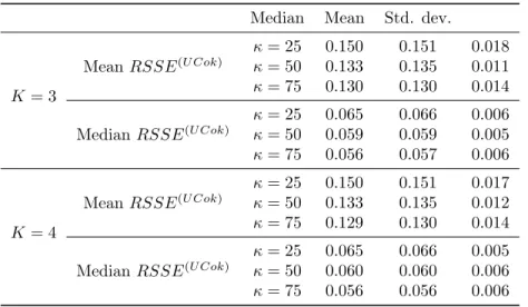
To evaluate the impact of the truncation orderKon the results, we repeated the same Monte Carlo analysis for K = 3,4. The results are listed in Table 2. Inspection of the entries of Table 2 suggests that the results for K = 3,4 are almost equivalent to those obtained with UTrK (Table 2), thus slightly improving the results for K = 2. No significant difference appears comparing the results corresponding toK = 3 and toK = 4, probably due to the small portion of variability explained by the fourth FPC. Even though the choice of
● ● ● ● ● UT rK: κ = 25 UT rK: κ = 50 UT rK: κ = 75 UCok: κ = 25 UCok: κ = 50 UCok: κ = 75 5 10 15 20 25 Mean RSSE RSSE [%] ● ● ● ● ● UT rK: κ = 25 UT rK: κ = 50 UT rK: κ = 75 UCok: κ = 25 UCok: κ = 50 UCok: κ = 75 0 5 10 15 Median RSSE RSSE [%]
Figure 9: Boxplots of RSSE indices for UCok and UTrK.
K = 2 can be considered as a fair balance between the problem complexity and the prediction performances, these additional results support the picture according to which the performances of UTrK and UCok methods are quite equivalent, provided that the retained components exhaustively represent the data variability. As such, the modeling and computational gain of UTrK over UCok is expected to be more relevant in the presence of data that require an elevate number of FPCs for a precise description.
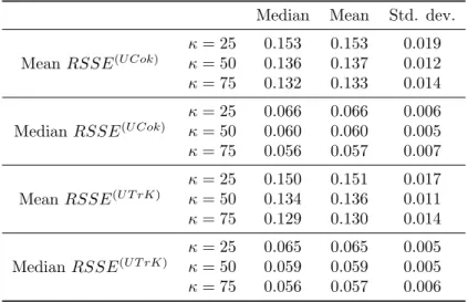
For sake of completeness, we report in Table 3 and Figure 10 the results obtained by projecting the log-GPRCs over the basis of the first two right func-tional singular vectors (FSVs), computed numerically. These are the equivalent, in the functional case, of the right singular vectors obtained in the well-known singular value decomposition (SVD) of a multivariate dataset. In this context and unlike FPCA, the procedure detailed in Subsection 2.1 can be applied with-out modifications,ek being represented by the k-th right FSVs.
We first notice that a significant number of upper outliers affects the results related to the mean RSSE(U Cok), for κ= 25. This is probably caused by an
amplification of the error due to the exponential transformation, as only one out-lier is recorded when SSE is evaluated on a log-scale. Besides this, simulations show that UTrK outperforms UCok in all the tested scenarios under FSVD pre-processing. In fact, marked differences are recorded between the performances of UCok under FPCA and of UCok under FSVD preprocessing. This is likely due to the fact that UCok under FPCA preprocessing is applied to centered observations, i.e., those obtained by subtracting the sample mean of the dataset from the observations (see the Appendix). In this sense, the entire information within the sample mean is kept in UCok prediction, as the latter is added to the UCok prediction obtained from centered data. In contrast, FSVD is applied to non-centered observations: here the dimensionality of the non-centered
obser-Median Mean Std. dev.
K= 3
MeanRSSE(U Cok)
κ= 25 0.150 0.151 0.018
κ= 50 0.133 0.135 0.011
κ= 75 0.130 0.130 0.014
MedianRSSE(U Cok)
κ= 25 0.065 0.066 0.006
κ= 50 0.059 0.059 0.005
κ= 75 0.056 0.057 0.006
K= 4
MeanRSSE(U Cok)
κ= 25 0.150 0.151 0.017
κ= 50 0.133 0.135 0.012
κ= 75 0.129 0.130 0.014
MedianRSSE(U Cok)
κ= 25 0.065 0.066 0.005
κ= 50 0.060 0.060 0.006
κ= 75 0.056 0.056 0.006
Table 2: Distribution of the RSSE indices for UCok based of FPCA withK = 3,4, in the original scale, assessed via Monte Carlo simulation.
Median Mean Std. dev.
MeanRSSE(U Cok)
κ= 25 0.170 0.528 3.198
κ= 50 0.148 0.163 0.080
κ= 75 0.141 0.144 0.019
MedianRSSE(U Cok)
κ= 25 0.070 0.070 0.007
κ= 50 0.063 0.063 0.006
κ= 75 0.060 0.060 0.009
Table 3: Distribution of the RSSE indices for UCok based of FSVD in the original scale, assessed via Monte Carlo simulation.
vations is reduced. Intuitively, givenK, FPCA exploits one dimension (that of the sample mean) more than FSVD, at the same expense.
These results underline the fact that, whenever a dimensionality reduction is performed prior to apply UCok, the prediction results may be influenced by the kind of dimensionality reduction method used (e.g., FPCA or FSVD) and the chosen dimension K. Such problem is overcome when using UTrK, as no preprocessing is required.
4. Conclusions
In this work, we considered two approaches to the spatial prediction of gas production rate curves (GPRCs) in unconventional reservoirs: (1) Universal Cokriging (UCok) and (2) Universal Trace-Kriging (UTrK). We analyzed the strengths and weaknesses of these methodologies both theoretically and from
● ● ● ● ● ● ● ● ● ● ● ● ● UT rK: κ = 25 UT rK: κ = 50 UT rK: κ = 75 UCok: κ = 25 UCok: κ = 50 UCok: κ = 75 5 10 15 20 25 Mean RSSE RSSE [%] ● ● ● ● ● ● UT rK: κ = 25 UT rK: κ = 50 UT rK: κ = 75 UCok: κ = 25 UCok: κ = 50 UCok: κ = 75 0 5 10 15 Median RSSE RSSE [%]
Figure 10: Boxplots of RSSE indices for UCok based on FSVD and UTrK.
the application viewpoint, through an extensive Monte Carlo study on field data.
The extensiveness of the considered dataset allowed us to perform exhaus-tive cross-validation analyses, with leave-out samples of considerable size (more than 200 samples). Even though we did not have a synthetic reference, results obtained from test sets of such sizes may be considered as reliable for this type of data. In addition to this, the consideration of real-world dataset allowed us to highlight the key points that one needs to address in a typical geostatisti-cal analysis of GPRCs (i.e., smoothing, modeling, prediction), and the actual potential of both methods on real data.
Our study shows that the investigated approaches lead to consistent results on available data. Nevertheless, UTrK proved preferable in some of the scenarios tested though Monte Carlo simulation. Here we showed that the dimensionality reduction operated on the data prior to the geostatistical analysis with UCok approach can be influential on the quality of the results. In this context, the simplicity of UTrK allows to avoid such preprocessing, and seems to be the key of its slightly better performances over UCok, obtained in some of the tested scenarios.
Anyway, we note that the theoretical study of UCok deserves attention from the methodological viewpoint. Indeed, UCok appears better suited than UTrK to extensions related to the form of the drift term. Indeed, one might want to consider a more complex functional linear model than that in Eq. (3). This would allow to incorporate geological or production variables, possibly time-varying (i.e., functional regressors), in the geostatistical analysis.
Appendix: Functional Principal Component Analysis
We here consider the Functional Principal Component Analysis (FPCA Ramsay and Silverman, 2005, Chapter 8) as a dimensionality reduction method for GPRCs, possibly log-transformed. FPCA is a methodology aiming to iden-tify a reduced space to optimally represent a set of observations. Given a tar-get dimension K, FPCA determines the system of K orthonormal directions
{ek,1≤k≤K} that best represents the variability of the data set around its mean.
As in the multivariate setting, the k-th Functional Principal Component (FPC) is the eigenfunction associated with the k-th largest eigenvalue of the (zero-lag) covariance operatorC(0), that isC(0)ek=ρkek,ρ1> ... > ρk. Note
that, in the assumptions of Section 2, all the data are featured by the same covariance operatorC(0).
The proportion of the variability explained by the firstK Functional Princi-pal Components (FPCs) can be measured through the ratio between the partial and the total sum of the eigenvalues ofC(0): PK
k=1ρk/P ∞
k=1ρk. To perform dimensionality reduction, one can then consider the projection of the data along the firstKFPCs,{ek,1≤k≤K}, whereKis set as to explain a given amount of the total variability (e.g., 90% or 95%).
If spatial covariance Cis unknown, one can introduce the empirical FPCA, that is based on the eigen-decomposition of the empirical zero-lag covariance operator, defined forx∈L2(T) as
b C(0)x= 1 n n X i=1 hXsi−X, xi(Xsi−X), (24) whereX =Pn
i=1Xsiis the sample mean (see, e.g., Horv´ath and Kokoszka, 2012,
Chapter 2.17). The coefficients for the basis representation are then obtained as ξek(si) = hXsi−X, eki, i = 1, ..., n, k = 1, ..., K. Notice that, if the mean
were spatially constant,X would estimate the mean of the process, andξek(si), i= 1, ..., nwould be zero-mean. In the non-stationary assumptions of Section 2,ξek(si) is not zero-mean, but approximately follows a model of the form (7), as we show below.
We callXesi,i= 1, ..., n, the modified dataset obtained by centering theXsi
with respect to the sample mean of the dataset, i.e., Xesi = Xsi−X. Under
models (3) and (5), for the modified processXesi one has
e Xs= K X k=1 L X l=0 akl fl(s)− 1 n n X i=1 fl(si) ! + K X k=1 k(s)ek− K X k=1 1 n n X i=1 k(si)ek. (25)
For a sample size sufficiently large with respect to K and a moderate spa-tial dependence (see Horv´ath and Kokoszka, 2012, Chapter 18), the last term becomes negligible, since {k(s)} is zero-mean. By noting that, given the re-gressors, Pn
obtained from expression (25) e Xs≈ K X k=1 L X l=0 aklfel(s) + K X k=1 k(s)ek. (26)
The latter term has the same form as Eq. (9), but with modified regressors. Notice in particular that model (26) is without intercept.
Therefore, when the dimensionality reduction is performed via the empirical FPCA, one can proceed as follows: (i) project theXesi,i= 1, ..., n, over the first
K eigenfunctions and compute the scores ξek(si), i= 1, ..., n, k = 1, ..., K; (ii) perform the geostatistical analysis/prediction of ξek(si) and obtain the UCok
prediction Xes∗0 at the target location s0 as described in Subsection 2.1; (iii)
compute the final prediction by adding to Xes∗
0 the sample mean X: X
∗ s0 = e X∗ s0+X. Acknowledgements
Authors would like to thank drillinginfo.com for generously providing aca-demic license/access to their website/database. Grujic and Caers would also like to acknowledge Stanford Center for Reservoir Forecasting (SCRF) consortium (2013-2015) for financially supporting this research.
References
Besse, P. C., Cardot, H., Faivre, R., Goulard, M., 2005. Statistical modelling of functional data. Applied Stochastic Models in Business and Industry 21 (2), 165–173.
Besse, P. C., Cardot, H., Stephenson, D. B., 2000. Autoregressive forecasting of some functional climatic variations. Scandinavian Journal of Statistics 27 (4), 673–687.
Caballero, W., Giraldo, R., Mateu, J., 2013. A universal kriging approach for spatial functional data. Stochastic Environmental Research and Risk Assess-ment 27, 1553–1563.
Chil`es, J. P., Delfiner, P., 1999. Geostatistics: Modeling Spatial Uncertainty. John Wiley & Sons, New York.
Cressie, N., 1993. Statistics for Spatial data. John Wiley & Sons, New York. Delicado, P., Giraldo, R., Comas, C., Mateu, J., 2010. Statistics for spatial
functional data. Environmetrics 21 (3-4), 224–239.
Giraldo, R., 2009. Geostatistical analysis of functional data. Ph.D. thesis, Uni-versitat Polit`ecnica da Catalunya, Barcellona.
Grujic, O., Da Silva, C., Caers, J., 2015. Functional approach to data mining, forecasting, and uncertainty quantification in unconventional reservoirs. In: SPE 174849, SPE Annual Technical Conference & Exhibition.
Henderson, B., 2006. Exploring between site differences in water quality trends: a functional data analysis approach. Environmetrics 17 (1), 65–80.
Horv´ath, L., Kokoszka, P., 2012. Inference for Functional Data with Applica-tions. Springer Series in Statistics. Springer.
Ignaccolo, R., Mateu, J., Giraldo, R., 2014. Kriging with external drift for functional data for air quality monitoring. Stochastic Environmental Research and Risk Assessment 28 (5), 1171–1186.
Josset, L., Ginsbourger, D., Lunati, I., 2015. Functional error modeling for uncertainty quantification in hydrogeology. Water Resources Research 51 (2), 1050–1068.
Kormaksson, M., Vieira, M. R., Zadrozny, B., 2015. A data driven method for sweet spot identification in shale plays using well log data. In: SPE Digital Energy Conference and Exhibition. Society of Petroleum Engineers.
Mant´e, C., Stora, G., 2012. Functional PCA of measures for investigating the influence of bioturbation on sediment structure. In: 20th International Con-ference on Computational Statistics. pp. 531–542.
Matheron, G., 1969. Le krigeage universel. vol. 1. Tech. rep., Fontainebleau: Cahiers du Centre de Morphologie Math´ematique, ´Ecole des Mines de Paris. Menafoglio, A., Guadagnini, A., Secchi, P., 2014. A Kriging approach based on Aitchison geometry for the characterization of particle-size curves in hetero-geneous aquifers. Stochastic Environmental Research and Risk Assessment 28 (7), 1835–1851.
Menafoglio, A., Petris, G., 2015. Kriging for Hilbert-space valued random fields: The operatorial point of view. Journal of Multivariate Analysis. DOI:10.1016/j.jmva.2015.06.012.
Menafoglio, A., Secchi, P., Dalla Rosa, M., 2013. A Universal Kriging predictor for spatially dependent functional data of a Hilbert Space. Electronic Journal of Statistics 7, 2209–2240.
Menafoglio, A., Secchi, P., Guadagnini, A., 2015. A Class-Kriging predictor for Functional Compositions with application to particle-size curves in heteroge-neous aquifers. Mathematical Geosciences. DOI:10.1007/s11004-015-9625-7. Mohaghegh, S., 2011. Modeling, history matching, forecasting and analysis of
shale reservoirs performance using artificial intelligence. In: SPE 143875, SPE Digital Energy Conference.
Mohaghegh, S., 2013. A critical view of current state of reservoir modeling in shale assets. In: SPE 165713, SPE Eastern Regional Meeting.
Mˇanescu, C. B., Nu˜no, G., 2015. Quantitative effects of the shale oil revolution. Energy Policy. DOI:10.1016/j.enpol.2015.05.015.
Nerini, D., Monestiez, P., Mant´e, C., 2010. Cokriging for spatial functional data. Journal of Multivariate Analysis 101 (2), 409–418.
Patzek, T. W., Male, F., Marder, M., December 2013. Gas production in the barnett shale obeys a simple scaling theory. PNAS 110 (49), 19731–19736. Ramsay, J., Silverman, B., 2005. Functional data analysis, 2nd Edition.
Springer, New York.
Sancho, J., Iglesias, C., Pi˜neiro, J., Mart´ınez, J., Pastor, J., Ara´ujo, M., Taboada, J., 2015. Study of water quality in a spanish river based on statis-tical process control and functional data analysis. Mathemastatis-tical Geosciences, 1–24. DOI:10.1007/s11004-015-9605-y.
Satija, A., Caers, J., 2015. Direct forecasting of subsurface flow response from non-linear dynamic data by linear least-squares in canonical functional prin-cipal component space. Advances in Water Resources 77, 69 – 81.
Ullah, S., Finch, C. F., 2013. Applications of functional data analysis: A sys-tematic review. BMC medical research methodology 13 (43), 1–12.
Vidic, R. D., Brantley, S. L., Vandenbossche, J. M., Yoxtheimer, D., Abad, J. D., 2013. Impact of shale gas development on regional water quality. Science 340 (6134).
Yan, F., Liu, L., Li, Y., Zhang, Y., Chen, M., Xing, X., 2015. A dynamic water quality index model based on functional data analysis. Ecological Indicators 57, 249 – 258.
Yang, W., M¨uller, H. G., Stadtm¨uller, U., 2011. Functional singular compo-nent analysis. Journal of the Royal Statistical Society: Series B (Statistical Methodology) 73 (3), 303–324.