Full-reserve banking (FRB) can be defined as a variety of arrangements which prohibit private

1

1 I

NTRODUCTION

Full-reserve banking (FRB) can be defined as a variety of arrangements which prohibit private money creation at least in the sense that the state would not guarantee repayment or par clearance of private monies or money-like assets (e.g. through deposit insurance or lender of last resort function to private agents). According to Dow et al (2015), today it would mean that banks could no longer create new money in the form of bank deposits in the process of bank lending. This can be

accomplished, for instance, by imposing 100% reserve requirement on banks’ demand deposits.1 FRB aims at separating the payments system from the financing system as well as monetary policy from credit policy.

After the global financial crisis, FRB became a topical issue as a potential solution to financial instability. It has been proposed, for instance, by two reports commissioned by the prime minister of Iceland (Sigurjonsson 2015; KPMG 2016), an established columnist at theFinancial Times

(Martin Wolf 2014a; 2014b), and Positive Money (Jackson and Dyson 2012); however, many economists and commentators judge FRB (either positively or negatively) without the use of a systematic analysis.

The scope of this paper is to investigate the economic consequences of money creation through government spending in a FRB system. It also briefly explores money creation under FRB through tax cuts, citizen’s dividend and quantitative easing. Furthermore, the paper studies under which circumstances credit crunches might occur in a FRB system. The examination of how economic agents could react to credit crunches is left out of this paper as there are several ways to address the issue and, therefore, it deserves its own study.

2

The specific contribution of this paper is to build the first post-Keynesian stock-flow consistent (SFC) model of FRB.2 _{FRB has not been previously modeled in a SFC framework popularized by} Godley and Lavoie (2012). Previously, it has only been modeled in a dynamic-stochastic general equilibrium framework (Benes and Kumhof 2012; 2013), in an overlapping-generation framework (Suntum and Neugebauer 2015), in a system dynamics framework (Yamaguchi 2010; 2011; 2014), in a dynamic simulation framework (Egmond and Vries 2015), and in a dynamic multiplier

framework (Flaschel et al. 2010; Chiarella et al. 2011). The last two of these come closest to SFC modeling being based on stocks and flows, but not in a complete and coherent way as in Godley and Lavoie (2012).

The SFC model of FRB built in this paper is called REFORM2. It is developed from Godley and Lavoie’s (2012) simple theoretical model INSOUT. According to Mäki (2011), even abstract and simplified models can be very insightful as what matters are the causal mechanisms at work and the resemblance of the model with respect to reality. INSOUT is a model that entertains all the standard post-Keynesian assumptions, such as endogenous money, a credit-led economy and exogenous interest rates on government debt. I would argue that the model is able to capture some essential elements of the current monetary economy.

There are only two major differences in REFORM2 besides other minor differences. First, it is assumed that the compulsory reserve ratio on demand deposits is equal to 100% instead of being only a fraction of it. Second, it is assumed that the amount of central bank money in the system is exogenous and hence that the interest rate on government bills is endogenous. The rigidity imposed by FRB is tamed by the added assumption that banks are quite happy to hold more than required compulsory reserves, within a certain band.

3

It is found that a stationary steady state exists. It is a necessary precondition for FRB to be

compatible with a zero-growth economy. Long-term economic growth is excluded from the model as there is no autonomously-growing demand component (e.g. investment in fixed capital or government expenditures).

The paper conducts an experiment in which money is created through government spending in a FRB system. The paper compares the time paths of variables to the cases in which government spending is increased under FRBwithout money creation and under endogenous money, that is, the current monetary system. To simulate the current monetary system the paper makes use of Godley and Lavoie’s (2012) model INSOUT from which the model REFORM2 is developed. There is sufficient resemblance to make a reasonable comparison.

It is found that under FRB, an increase in government spending which is financed with money creation leads to a temporary increase in output, employment and inflation. The evolvement of these variables is practically identical also when government spending is increased under FRB without money creation and under the current monetary system. Unlike in other cases, however, money creation in a FRB system leads to a permanent reduction in consolidated government debt. An increase in central bank reserves translates into an almost equal increase in demand deposits. Furthermore, an unusually large change in the money supply only leads to smooth and relatively small changes in interest rates.

In addition, the paper compares three additional ways to create money. Money creation through reducing taxes or paying a dividend for citizens yields roughly similar results than creating money through government spending. Contrastively, creating money through quantitative easing affects

4

only monetary aggregates and interest rates but not the real economy. As the effects of money creation vary according to the channel, money creation under FRB would require some coordination between the government and the central bank. In other words, the appropriate amount of new

money should depend on how it enters the economy.

Finally, the paper explores the circumstances under which FRB might lead to a credit crunch. Although in every money creation experiment banks are able to satisfy the demand for loans, temporary credit crunches can occur due to changes in private behaviour such as a sudden increase in liquidity preference or demand for loans. In addition, credit crunches can be induced by

contractionary monetary or fiscal policy. The susceptibility of credit crunch depends on the magnitude of changes and the safety margins adopted by banks.

A more elaborate model would shed more light on the likelihood of credit crunches. Introducing fixed capital, productivity growth or lower bank liquidity target would increase the likelihood of credit crunches. Ultimately, the only way to ensure that FRB would not cause credit crunches would be to allow banks to borrow reserves from the central bank, but this would reduce the ability to control the money supply.

The paper is structured as follows. Section 2 presents the balance sheet and transaction-flow matrices. Section 3 presents and explains the equations. Section 4 discusses the calibration process and the properties of the “old” steady state. Section 5 conducts an experiment in which government spending is increased under FRB with and without money creation as well as under the current monetary system. In addition, the section briefly investigates other options for money creation. Section 6 explores the circumstances when FRB might cause a credit crunch. Finally, section 7 concludes.

5

2 M

ATRICES

This section presents the matrices of the model REFORM2. The first subsection presents the balance-sheet matrix. The second subsection presents the revaluation matrix. Finally, the third subsection presents the transaction-flow matrix.

2.1 B

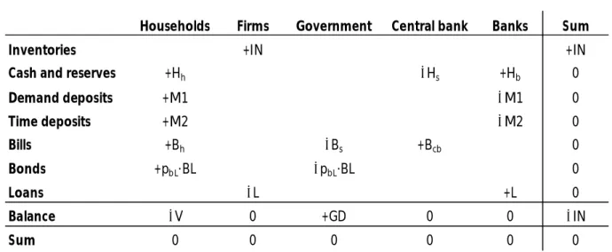
S

This subsection presents the balance-sheet matrix for the model REFORM2. The table below depicts all real and financial assets and liabilities each sector can hold. Naturally, all columns and rows sum to zero except for real assets (inventories).

[Insert Table 1]

The balance sheet matrix of REFORM2 is very similar to the balance sheet matrix of INSOUT in Godley and Lavoie (2012). Households hold cash, demand deposits, time deposits, government bills, and government bonds. Firms finance their inventories (working capital) with bank loans. Fixed capital is omitted. The government finances its budget deficit by issuing bills and bonds. The central bank buys government bills in order to issue cash and reserves. Banks hold reserves and loans as assets and demand and time deposits as liabilities. Thus, the model is, effectively, a combination of the Chicago Plan (demand deposits held with banks) and sovereign money (banks can make loans by issuing time deposits).

6

The only differences between REFORM2 and Godley and Lavoie’s (2012) INSOUT model are that banks do not hold bills and banks do not have access to central bank advances.

Government bonds are the only asset of which value can change between periods as in Godley and Lavoie’s (2012) model INSOUT. Bonds are long-term securities here defined as perpetuities (also called consols) because they are never redeemed. It is assumed that each perpetuity pays the owner one unit of currency (e.g., dollar) after one period has elapsed. The one unit of currency is the coupon of the perpetuity. Bills are assumed to be short-term securities that mature within each period; therefore, their value cannot change between periods.

2.2 T

F

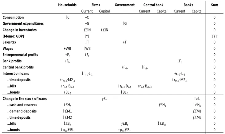
This subsection presents the transaction-flow matrix for the model REFORM2. The table below presents the transaction-flow matrix, which captures all transactions and flows between sectors and between periods. Thus, what happens within a sector or within a period is not depicted. As usual, all the rows and columns of the transaction-flow matrix sum to zero.

[Insert Table 2]

The upper part of the transaction-flow matrix is the national income part. The key features are that only sales are taxed (no income tax) and all profits are always distributed (no retained earnings). GDP is added only as a memo item for clarification.

7

The lower part of the transaction-flow matrix is the flow-of-funds part which records change in financial assets. The changes must exactly match the national income part. For example, if households have more inflows than outflows in the national income part, they are saving. In the flow-of-funds part this means that they are accumulating at least one type of asset (which is recorded with a minus sign in order to balance the column).

The national income part of the transaction-flow matrix (the upper part) is exactly the same as in Godley and Lavoie’s (2012) model INSOUT. The only differences in REFORM2 are that there are no changes in the stocks of advances or bills held by banks (as banks do not hold advances or bills) and, thus, there are, of course, no interest payments on central bank advances or on banks’ holdings of bills either.

3 E

QUATIONS

This section presents the equations of the model REFORM2. In total there are 80 equations of which 74 enter the model. The equations of firms and some of the equations of households are put in an appendix as they are almost straightforward replications of Godley and Lavoie’s (2012) model INSOUT.

It should, however, be stated that equations alone are insignificant. What matters are the underlying theories, which try to shed light on how the economy functions. The equations described in this section convey many elements from post-Keynesian economic theory as well as more specific theoretical elements related to money and banking.

8

The notation of equations follows that of Godley and Lavoie (2012). Thus, for readers ofMonetary Economics this section should be quite easy to follow.

Capital letters denote nominal values while lower case letters denote real (inflation accounted) values. Greek letters are parameters.

Subscript–1 refers to the end of previous period value (starting value for the current period). Subscriptss andd refer to supply and demand, respectively, in a broad sense. Subscriptsf,h,g,cb,

andb refer to different sectors: firms, households, government, central bank, and banks, respectively. Variables without subscript refer to realized values.

Superscripte refers to short-term expected or target value while superscriptT refers to long-term target value. Short-term and long-term target values differ as short-term targets typically follow a partial adjustment process. That is, economic agents do not try to immediately (within one period) reach their term targets, but instead slowly adjust their short-term targets towards their long-term targets.

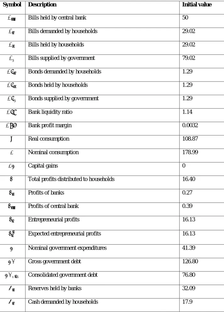
SuffixA in the numbering of equations denotes that the equation is dropped from the model either because it is redundant or it is there only for clarification. All endogenous variables are allowed to appear only once on the left-hand side of an equation. The full list of variables with (initial) values is provided in the second appendix.

3.1 H

9 = + + ∙ 2 + ∙ + (H.1) = (∆ )∙ (H.2) = + (H.3) = + (H.4) = + − (H.5) = + 1 + 2 + + ∙ (H.6A) = − (H.7) = − ∙ (H.8) = + (H.9) = + ∆ (H.10A) = (H.11)

Unlike with firms, I describe the equations for households starting from realized outcomes and only then proceeding to decisions. Regular disposable income includes wages, profits, and interest revenue on time deposits, bills, and bonds (H.1). Capital gains are the change in the price of bonds multiplied by the end-of-period amount of bonds (H.2). Haig-Simons nominal disposable income includes regular disposable income and capital gains (H.3). Total profits distributed to households consist of entrepreneurial profits and banks’ profits (H.4). Notice that profits are always distributed in full and, therefore, there are no retained earnings.

Wealth of households is the wealth inherited from the previous period plus Haig-Simons disposable income minus consumption (H.5). Wealth of households could also be written as the sum of all financial assets (H.6A), but as will be later seen this equation is saved for another purpose. Wealth of households expressed as net of cash will be useful in portfolio equations (H.7). Real regular disposable income is nominal regular disposable income minus the inflation tax on real wealth

10

(H.8). Similarly as before, Haig-Simons real disposable income is real regular disposable income plus real capital gains (H.9), which is the same as real consumption plus the change in real wealth (H.10A). Real wealth is, of course, nominal wealth divided by the price level (H.11).

The equations of households describing the decision-making process and the demand for assets (H.12 to H.22) can be found in the appendix.

Realized asset holdings:

= (H.23) 1 = −( 2 − ) (H.24) 2 = 2 (H.25) = (H.26) = − − 1 − 2 − ∙ (H.27) = − (H.28A) = ∙ ∙ ∙ (H.29)

Although portfolio equations determine the demand for assets, the realized holding of some assets differs as realized wealth and income usually differ from what was expected. The realized holding of cash, however, is exactly equal to its demand (H.23).

As in Godley and Lavoie (2012), demand deposits act as a “buffer” which reconciles the

discrepancy between expected and realized outcomes. The realized holding of demand deposits is determined by central bank reserves minus the difference between time deposits and loans (H.24). This can also be read from banks’ balance sheet. The idea behind this is that demand deposits are initially equal to reserves. However, households can invest in time deposits offered by banks, which

11

reduces demand deposits held by households. Banks’ can now use these funds to make loans. As banks make loans, demand deposits are returned into circulation (thus, bank lending does not create money under FRB). If banks do not make loans as much as households make time deposits, demand deposits do not get returned into circulation and, therefore, their amount is less than reserves.

Time deposits and bonds are determined more straightforwardly. The realized holdings of time deposits and bonds equal their demand (H.25 and H.26).

The realized amount of bills held by households is total wealth minus other financial assets (H.27). This equation is simply (H.6A) rearranged. However, the amount of bills left for households is entirely determined by the decisions of the government (how many bills it issues) and the central bank (how many bills it buys to monetize government debt) (H.28A). In other words, households are the residual buyer of bills. Nevertheless, households cannot be forced to hold bills against their will.

In order to ensure that households buy exactly all the remaining bills, the interest rate on bills must be endogenous (also shown by Godley and Lavoie 2012 in the Appendix of Chapter 4). Thus, the interest rate on bills, rb, is determined by the portfolio equation (H.21A) solved for the bill rate instead of the amount of bills (H.29). In the model the bill rate is the benchmark interest rate which banks use as a basis for setting their loan rate.

The redundant equation is the equation indicating that households are the residual buyer of bills (H.28A). Although equation (H.28A) does not explicitly enter the model, it gives exactly the same result as (H.27). The equation is dropped from the model as otherwise the model would be

12

overdetermined. This means that all the other equations together already imply the dropped equation.

3.2 G

The government collects taxes according to the sales tax rate it sets exogenously (G.1). Nominal government expenditures are simply real government expenditures, which are set exogenously, multiplied by the price level (G.2).

The government budget deficit, that is, the public sector borrowing requirement (PSBR) is the difference between total outlays (including spending and interest payments on bills and bonds) and total income (including taxes and central bank profits) (G.3). The government issues (redeems) bills to finance the part of the budget deficit (surplus) that is not financed by the issuance of government bonds (G.4). The government lets households decide how many bonds they want to hold (G.5) with

13

the interest rate set exogenously by the government (G.6). The price of bonds is simply the coupon (one unit of currency) divided by the bond rate (G.7).

Gross government debt4is simply the value of outstanding bills and bonds (G.8). Consolidated government debt5 is the value of bills and bonds held by non-public entities (G.9). Put differently, consolidated government debt is gross government debt minus intra-government debt (in this case bills held by the central bank). Consolidated government debt can alternatively be called as net government debt.

3.3 C

B

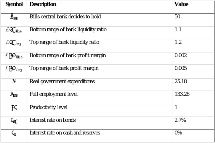
The central bank can greatly influence the money supply through reserves. As can be directly read from the balance-sheet matrix, the central bank sets the amount of reserves by determining how many bills it holds (C.1). The simplest monetary policy rule is to keep the amount of bills constant, that is, the amount of bills is exogenous (C.2). Alternative monetary policy rules are worth

considering but they are not the topic of this paper.

As it is assumed that interest is not paid on cash or reserves (C.3), the profit of the central bank is determined by the interest payments it receives on bills from the government (C.4).

14

3.4 B

The full-reserve requirement is incorporated by setting the reserve requirement for demand deposits equal to 1 (B.1). There is no reserve requirement for time deposits so is equal to zero. Banks hold whatever reserves they are left with after the central bank has decided the amount and

households have satisfied their demand for cash (B.2). The bank liquidity ratio is the ratio between reserves held by banks and required reserves (B.3). Under FRB this ratio has to be at least 1.

Monetary and credit aggregates:

1 = 1 (B.4)

2 = 2 (B.5)

= (B.6)

Banks supply both demand and time deposits in whatever amount is required (B.4 and B.5). As previously described, the amount of demand deposits can be read from the banks’ balance sheet (H.24). The amount of time deposits is completely determined by their demand (H.20 and H.25). Banks also accommodate the demand for loans for all creditworthy firms (B.6).

15 = + ∆ (B.7) ∆ = ∙( − ) (B.8) = 1, < (B.9) = 1, > (B.10) = + ∆ + ∆ (B.11) ∆ = ∙( − ) (B.12) = 1, < (B.13) = 1, > (B.14) = (B.15) = ∙ − ∙ 2 (B.16)

Banks can set the interest rates on time deposits and loans, while the interest rate on demand deposits is assumed to be zero (which is also very much in line with the real world today). Banks follow a partial adjustment process when setting the interest rate on time deposits (B.7 and B.8). If the bank liquidity ratio falls below its desired level in the previous period, banks increase the deposit rate to attract more time deposits (B.9). As households invest in time deposits, their demand deposits get reduced and this increases the bank liquidity ratio. Symmetrically, when the bank liquidity ratio increases above its desired level in the previous period, banks decrease the deposit rate to reduce the amount of time deposits (B.10). As long as the bank liquidity ratio stays within its desired range, banks do not alter the interest rate on time deposits.

Banks set the interest rate they charge on loans to ensure a sufficient profit margin. When setting the loan rate, banks follow the bill rate and a partial adjustment process (B.11 and B.12). Now, when the bank profit margin is below its desired level, banks increase the interest rate they charge on loans (B.13). Symmetrically, when the bank profit margin is above its desired level, banks decrease the interest rate on loans (B.14). Unlike in mainstream economics, banks do not maximize

16

profits (at least in the short run). Godley and Lavoie (2012, 340) justify this by the banks’ fear of government regulation or consumer outrage. The bank profit margin is determined by average profits divided by the sum of average demand and time deposits (B.15). Finally, banks’ profits are determined by the difference between the interest payments they receive from loans and the interest payments they make on time deposits (B.16). In this model real rates are meaningless but they could be used instead of nominal rates.

4 C

ALIBRATION

AND

S

TEADY

S

TATE

In the simplest SFC models it is possible to obtain a determinate analytical solution for a steady state. However, in more complex models, such as REFORM2, obtaining a determinate steady-state solution analytically becomes impossible as the model is path-dependent. It can be said that the model exhibits deep endogeneity as the steady state depends on the past history. The solution for each set of parameters, exogenous variables and initial stock values can, however, be obtained through simulation.

Before going to the simulation results, it is explained how the model was calibrated. First, all values of parameters, exogenous variables and initial stocks (of endogenous variables) were directly adopted from Godley and Lavoie’s (2012) model INSOUT. Then, some of them were adjusted to yield a suitable solution. That is, the simulation yielded a steady state, no negative values existed for any variable and stock values were convenient (e.g. all monetary aggregates were at least 10). Then, initial stock values were updated from the end values of the previous simulation (in which variables might fluctuate in the early periods) so that the system is at its steady state already from the first period onwards.

17

Now, the properties of the steady state are presented. The steady state of REFORM2 is stationary, that is, the levels of key variables remain constant. Long-term economic growth is excluded from the model as there is no autonomously-growing demand component. Stationary steady state is a necessary precondition for FRB to be compatible with a zero-growth economy.

In the steady state both full employment and zero inflation are sustained. In addition, there is no increase in either public or private debt. Servicing debt is also entirely possible.7 _{Banks are able to} supply all loans that are demanded by creditworthy borrowers. In the long run the availability of loans is secured as banks adjust the interest rate on time deposits to attract enough deposits to fund the loans.

The existence of a steady state in an FRB system implies that the system can be attained indefinitely. However, it is possible that the system becomes unstable as soon as something changes. Next, in order to address this issue, let us conduct money creation experiments with the model REFORM2. Later, the possibility of a credit crunch is considered.

5 M

ONEY

C

REATION

THROUGH

G

OVERNMENT

S

PENDING

Under FRB money can be created through government spending, as has been proposed by Jackson and Dyson (2012) and Sigurjonsson (2015) among others. This section compares what happens when government spending is increased under FRB – with and without money creation – and under endogenous money, that is, the current monetary system. FRB with money creation refers to an increase in government spending financed by the purchase of government securities by the central

18

bank. Contrastively, FRB without money creation means that government spending is financed by issuing bills and bonds to the market. FRB is studied with the model REFORM2 described in the previous sections while endogenous money is studied with the model INSOUT (full description of the model can be found in Godley and Lavoie 2012, Ch. 10).

In all cases, real government spending is temporarily increased by 36% for one period and then returned to its original value (initially public expenditures account for 19% of GDP). Under FRB with money creation, the government increases its spending in nominal terms by 15. At the same time, the central bank buys bills worth 15 which increases reserves by 15. The increases are 7% of GDP.

The increase in government spending takes place in period 6. For clarification, the following subsections use notationt=0 for indicating period 6, that is, exactly when government spending takes place,t=1 for the following period, etc.

When interpreting the figures, it is important to take the scale into account as the figures are scaled appropriately to depict the movements of variables. Therefore, depending on the scale, a radical-looking movement can be insignificant and, vice versa, a minor-radical-looking movement can be very significant.

19

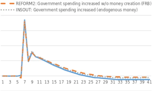
As can be seen from Figure 1, below, the development of output, employment and inflation is very similar under FRB – either with or without money creation – and under the current monetary system. Real GDP, employment and inflation speed up temporarily after government spending is increased. The level of real GDP peaks at a 7% higher level and then returns to its “new” steady state value which is exactly the same as the “old” steady state (in the figure the initial levels are normalized to 1).

[Insert Figure 1]

The development of employment resembles very closely the development of output (in the figure employment is compared to the “old” steady state). This is completely in line with post-Keynesian economic theory as post-Keynesians often maintain that employment is mainly determined in the product market rather than in the labour market. Also employment peaks at a 7% higher level before converging back to the original level as the effect of government spending stimulus fades away.

The period-on-period inflation rate peaks at 0.5% before returning to zero in the “new” steady state. In the peak the price level is 3% higher, but as inflation is very slightly negative for multiple

periods, the price level also ultimately converges to its “old” steady-state value.

The identical development of output, employment and inflation in all cases might strike somebody as surprising. However, it is completely in line with post-Keynesian literature as what matters are

20

stocks and flows. FRB or money creation under it does not in itself create any additional income or expenditure flows and thus significantly alter, for instance, consumption or investment decisions (government spending decision is made identical in all cases by design).

5.2 G

D

D

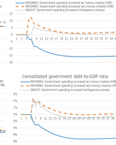
As post-Keynesians often emphasize, relying on an accounting identity, public sector debt increases private sector wealth. The net financial wealth of the whole private sector – comprising households, firms, and banks – is exactly equal to gross government debt (when the foreign sector is excluded as is the case here). Figure 2 shows the government deficit in absolute terms and the development of bills and government debt compared to the “old” steady state.

[Insert Figure 2]

In all experiments the government runs a brief but large budget deficit followed by a persistent but small budget surplus. Not surprisingly, gross government debt first increases and then slowly reverts back in all cases. As pointed out, this also represents the development of the net financial wealth of the private sector. The temporary increase in net financial wealth encourages households to consume more (wealth enters the consumption function as equation H.12 indicated), but when gross government debt is reduced also consumption returns to its “old” steady state level.

21

However, more interesting is the smooth and permanent reduction in consolidated government debt under FRB when government spending is financed with money creation. The consolidated

government debt-to-GDP ratio drops by 7 percentage points which is exactly equal to the amount new money was created.

It has at least three implications. First, it reduces interest payments on government debt which can be used otherwise to service the public interest.

Second, it allows fiscal stimulus while simultaneously reducing the relevant measure of government debt. The same result could, of course, be accomplished in the current monetary system too if the government engages fiscal stimulus while at the same time the central bank executes quantitative easing by buying government debt.

Third, in the long run after more and more money was created the government could also become “debt-free,” if so decided, in the sense that it would not be indebted towards any private agent. As Fontana and Sawyer (2016) point out, this, however, is not necessarily desirable as there is a recognized demand for risk-free financial assets bearing interest.

Another interesting issue is that under FRB with money creation bills held by households decrease – and they keep on decreasing over multiple periods even after the government does not receive any additional funds from money creation (notice that all government debt is held in the form of bills and bonds). In the experiment the central bank buys bills worth 15, the government increases its

22

spending by 15 for one period, and then government spending returns to its previous value. Intuitively, the amount of bills held by households should stay constant as households are the residual buyer of bills.

The counterintuitive result can be explained as follows. As some of the government spending also increases tax revenue for the government, the government budget deficit is less than 15, that is, less than the increase in government spending (this is true also for the other cases as the figure above indicates). Although originally the government issues new bills worth 15, additional tax revenue is collected already during the accounting period and by the end of the period 6 (t=0) government bills have only increased by 12. Under FRB with money creation this leads to the situation where

households’ holding of bills is reduced by 3 during period 6 (t=0) as the central bank buys 15 of them.

In periods 7 and 8 (t=1–2) households reallocate their wealth and increase their holdings of bonds of which the interest rate remains unchanged (not depicted in a figure). This further reduces the amount of bills households hold as government debt can be restructured by households; that is, an increase in bonds means an equal decrease in bills (given the amount of government debt), as can also be read from equation (G.4).9

From period 7 onwards (t=1+), the government runs a small but persistent budget surplus which also partly reduces bills and bonds held by households. Finally, the economy finds the “new” steady state where households have reduced their holding of bills by 16.

23

Under FRB with no money creation the consolidated government debt-to-GDP ratio moves in tandem with the gross government debt-to-GDP ratio. Also under endogenous money the

developments are similar although the central bank has to buy part of the newly issued bills in order to keep the interest rate on bills constant. This explains why consolidated government debt is in the end slightly lower under endogenous money than under FRB without money creation.

Even though output, employment and inflation evolved very similarly across experiments (see Figure 1), FRB could generate more capacity for fiscal policy. As Figure 2 showed, consolidated government debt decreases under FRB when new money creation occurs. In other words, FRB could increase the fiscal space of governments (a similar result could be achieved under the current monetary system too should the central bank monetize fiscal stimulus). In particular, when these reductions in consolidated government debt accumulate over time, this can, potentially, allow more emancipatory economic policies although, obviously, they are not an automatic consequence of FRB.

5.3 M

C

A

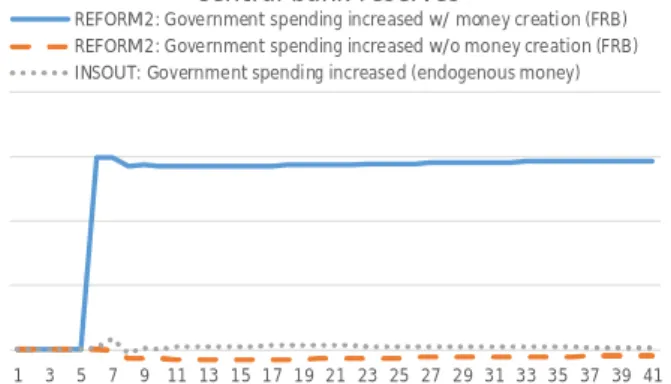
Figure 3, below, shows the evolution of central bank money compared to the “old” steady state. Central bank money is the sum of cash and reserves. Notice that under FRB the amount of central bank money is in total control of the central bank while under the current monetary system the amount of central bank money is determined endogenously.

24 [Insert Figure 3]

The amount of cash barely changes as its demand is a tenth of consumption (notice the scale). It also evolves very similarly in all cases as consumption develops similarly.

Under FRB when money is created central bank reserves held by banks permanently increase by 15. The reason is that money creation, which in this experiment finances the increase in government spending, takes the form of central bank money. The small fluctuation in reserves is due to substitution between cash and reserves. In the other two cases, the amount of reserves hardly changes.

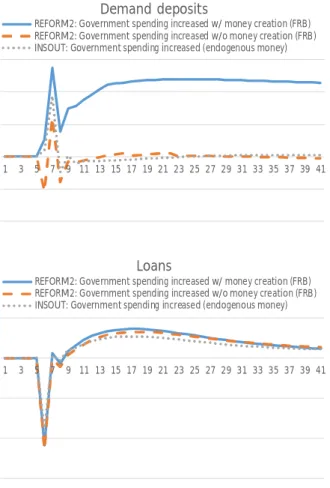
Figure 4, below, indicates the development of demand deposits, time deposits and loans relative to the “old” steady state. In all cases demand deposits fluctuate in a parallel direction but they

permanently remain on a higher level only under FRB with money creation while in the other two cases they return to their initial level.

[Insert Figure 4]

In all cases demand deposits act as a “buffer” and their amount is determined as a residual. As equation (H.24) indicated, demand deposits held by households depends on reserves and the

discrepancy between time deposits and loans. Should time deposits and loans stay constant or move by the same amount in the same direction, changes in demand deposits would exactly match

25

changes in reserves. However, this is not the case, as households will reallocate their wealth and firms will adjust their demand for loans.

Under FRB with money creation the reason why an increase in reserves does not instantly translate into an equal increase in demand deposits is that households and firms adjust their behaviour gradually. In typical neoclassical models agents have rational expectations, that is, they can foresee the future and therefore adjust their behaviour accordingly. This is generally not the case in post-Keynesian economics as agents have adaptive expectations and expectations are not normally realized.

Finally in the “new” steady state, all monetary and credit aggregates level off (there are only very minor movements as variables continue to converge to their ultimate values). In the end, under FRB with money creation, after increasing reserves by 15, demand deposits increased by 12, time

deposits by 4, and loans by 1. To put it briefly, increasing central bank money under FRB translates into an almost equal (80%) increase in demand deposits.

The next subsection discusses how interest rates (are) adjust(ed) as a reaction to changes in monetary and credit aggregates.

26

Perhaps the most significant differences between the experiments can be found in interest rates. Figure 5 depicts the development of interest rates on government bills, loans and time deposits relative to the “old” steady state. The interest rate on government bills is the main interest rate in all cases.

[Insert Figure 5]

The determination and development of the bill rate varies across experiments. In a FRB system the bill rate is determined endogenously as equation (H.29) revealed. As the central bank sets the amount of central bank money by buying or selling government bills and households are the residual buyer of bills, the bill rate has to adjust in order to reconcile demand with supply.

Contrastively, in the current monetary system the bill rate is the target policy rate and therefore it is set exogenously by the central bank. Thus, it is the amount of bills that has to adjust. This is also the reason why the bill rate does not react to any changes in government spending under endogenous money.

Under FRB the bill rate moves in tandem with the amount of bills held by households. If money is not created, the government has to issue more bills to households in order to finance the increase in expenditure. Households are only willing to buy the additional bills if their return is higher. Thus, the bill rate temporarily increases.

27

However, under FRB with money creation the bill rate drops to a permanently lower level. As explained in Subsection 5.2, the bill rate drops immediately after government spending is increased as the budget deficit is less than the amount that central bank monetizes government debt. In other words, as households are left with fewer bills, the interest rate on bills drops slightly to reconcile demand with supply. The subsequent decrease in the bill rate follows the same rationale as discussed in Subsection 5.2.

The interest rate on loans is determined in the same way in all experiments. The loan rate depends on the bill rate and banks further adjust it according to their profit margin. Under FRB without money creation the bank profit margin remains within its target range and, consequently, the loan rate is a pure reflection of the development of the bill rate.

Under FRB with money creation, however, the bank profit margin drops below its bottom range. Thus, the interest rate on loans is adjusted upwards and it does not simply follow the bill rate. In the end, the loan rate settles to a slightly lower level. The main reason for the drop in bank profitability is that the amount of time deposits increases and, thus, banks have to pay more interest to

depositors. Also the sharp drop in the amount of loans reduces the income stream of banks although the drop is only very brief as the amount of loans recovers quickly.

Under endogenous money the loan rate goes in the opposite direction. The bank profit margin increases above its top range and, therefore, banks temporarily lower the loan rate. Nevertheless, this reduces bank profits and eventually banks adjust the loan rate back to its initial level. The reason for the temporary increase in bank profitability are changes in bank balance sheet, chiefly, as

28

they acquire more bills (which is not allowed in REFORM2), and because the interest rate on time deposits drops.

Finally, let us examine the development of the interest rate on time deposits. In all experiments the driving force is bank liquidity. The definition of bank liquidity, however, differs. In REFORM2 the bank liquidity ratio was defined by equation (B.3) as reserves relative to demand deposits. Under FRB this ratio has to be at least 1 to satisfy the liquidity requirement. In the model banks have a safety margin as their target range is 10–20% above the requirement. In INSOUT the bank liquidity ratio is defined in terms of government bills held by banks relative to both demand and time

deposits. Moreover, in INSOUT also the bill rate has a proportional impact on the deposit rate (although the bill rate is exogenous and, thus, does not change in the experiment).

Under FRB banks can indirectly influence their liquidity ratio by changing the interest rate they offer on time deposits. This can partly help to explain the above-observed fluctuations in time deposits.

Under FRB with money creation the adjustment process goes as follows. The central bank injects extra liquidity into the banking system. Banks react to this by reducing the interest rate on time deposits to curb households’ demand for them. Banks lower the deposit rate in steps for multiple periods until their liquidity ratio is within the desired range.

29

In the other two cases the interest rate on time deposits first drops and then increases above the initial level. In both cases the liquidity of banks first increases although due to different reasons. Under FRB without money creation demand deposits decrease while under endogenous money government debt increases which leaves the banks with more bills. Subsequently, in both cases the liquidity of banks decreases and banks hike up the deposit rate – again for different reasons. Under FRB without money creation the reason is that demand deposits recover and increased demand for cash reduces central bank reserves held by banks while under endogenous money the government surplus reduces the amount of bills held by banks. Eventually, in both cases the interest rate on time deposits ends up slightly above the initial level.

According to the experiments above, in contrast to what some claim (e.g. Dow et al 2015; Dittmer 2015; Fontana and Sawyer 2016), FRB does not lead to excessively volatile interest rates. Both experiments with FRB led to a smooth and relatively small change in the bill rate on its path to its “new” steady-state value (under the current monetary system the bill rate was exogenous and thus constant by design). Surprisingly, interest rates on loans and time deposits were actually more volatile in the current monetary system than in a FRB system. Therefore, the fear that FRB would destabilize interest rates seems exaggerated.

5.5 O

O

M

C

In addition to government spending new money into circulation, Jackson and Dyson (2012) and Sigurjonsson (2015) give three additional ways to create money in a FRB system: reduce taxes; pay dividend for citizens; and repay government debt (i.e. quantitative easing). This subsection

30

compares these alternative options to create money to the case when new money was created through government spending.

Reducing taxes yields very similar – although more turbulent – results than when new money is created through government spending. Notice that only firms are taxed in the model so that the tax cut is a temporary reduction to firms’ sales tax from 24.2% to 15.7% for one period. The most significant difference is that especially the inflation rate fluctuates more. Both inflation and deflation peak at 6% while in the previous case period-on-period inflation peaked at a mere 0.5%. Ultimately, however, the price level returns to its previous level as it did when money was created through government spending.

Again, creating new money through a one-shot citizen’s dividend, advocated by Joan Robinson (1937) among others, the dynamics are very similar.8 _{Unlike in the previous cases, however, the} government has to borrow exactly the same amount than new money is created. That is, the government budget deficit peaks at 15 while in the previous cases the deficit peaked at 12. The reason is that in the previous cases some of the stimulus is returned in the form of higher tax

revenue already within the accounting period when new money was created. In this case households alter their behavior only in the following periods due to recursive expectations. Introducing more simultaneous or forward-looking expectation formation or consumption decision for households would, of course, mean that part of the stimulus is returned as higher tax revenue already within the accounting period.

Whennewmoneyiscreatedthroughquantitativeeasing,governmentdebtismonetizedwithoutany stimulus(exceptperhapsthroughlowerinterestrates).Contraryto the previous experiments,

31

on the real economy. If not accompaniedwithfiscalstimulus,quantitativeeasingaloneisnotenough tostimulatetherealeconomyunderFRB(astheaftermathoftheGFCshowed,thisseemstobeoften thecasealsointhecurrentbankingsystem).

6 C

REDIT

C

RUNCHES

In all the previous money creation experiments banks were always able to supply all demanded loans and, thus, there were no credit crunches. Although it caused some fluctuations to the banks’ liquidity ratio, money creation under FRB did not impose any serious threats to the full-reserve requirement. However, this is not always the case.

Basically, a credit crunch can occur under FRB due to two reasons: liquidity or funding. There can be insufficient liquidity if either reserves held by banks drop or demand deposits supplied by banks increase and, consequently, the FRB requirement is violated. Funding can cause trouble if banks are unable to finance their loans as the demand for loans increases or the amount of time deposits drops. By implication, these two reasons are the same in the model REFORM2: if there is insufficient liquidity, there is also insufficient funding (see Table 1). This, however, is not necessarily the case in reality as banks hold a variety of assets although liquidity and funding are often interrelated also in that case.

This section studies the conditions and mechanisms of potential credit crunches under FRB with the model REFORM2. In the steady state (or in the long run) the banks’ liquidity target ensures that

32

banks respect the FRB requirement. Nevertheless, in the short run it is possible that banks have to limit their supply of loans or the economy has to adjust otherwise in order to avoid the violation of the FRB requirement.

In this section I will, first, study how the private sector can cause credit crunches. Second, I examine how economic policy, in particular, monetary and fiscal policy can cause credit crunches. Finally, I discuss how the economy can cope with and possibly even avoid credit crunches under FRB.

6.1 P

B

This subsection experiments how a change in private behaviour can induce a credit crunch. More precisely, the subsection examines with the model REFORM2 how certain exogenous parameters should change so that there would be a credit crunch. In the first two experiments households’ liquidity preference is increased while in the third experiment firms’ demand for loans is raised.

In the first experiment households’ liquidity preference increases as they demand more cash. This drains reserves from the banking system which are used for 100% backing of demand deposits. A credit crunch would occur if households would like to increase their holding of cash from 10% to 13.2% compared to their consumption. In other words, a credit crunch occurs should households suddenly like to hold 32% more of cash than previously.

33

Also in the second experiment households’ liquidity preference increases but, instead of cash, they desire more demand deposits. Instead of draining reserves from the banking system, this increases the amount of reserves banks are required to hold (while the amount of reserves is not altered). As equation (H.24) indicated, demand deposits held by households can only be affected indirectly. In this experiment demand deposits increase as the demand for time deposits decreases (i.e.

households withdraw time deposits and receive demand deposits in return). Banks would have to limit their supply of loans if households would suddenly like to shift 3% of their wealth (net of cash) from time deposits to demand deposits. This means that households would like to hold 18% more demand deposits and 9% less time deposits.

In the third experiment firms demand more loans. As equation (H.24) shows, this adds demand deposits into the economy and, again, they are required to be fully-backed by reserves. In this experiment the demand for loans is increased through an increase in firms’ targeted inventories. It turns out that it would be enough to induce a credit crunch if firms suddenly want to raise their target inventories-to-sales ratio by 5% points. This would translate into a 16% increase in desired inventories which also means that the demand for loans increases by 16%.

6.2 M

F

P

This subsection examines how contractionary monetary and fiscal policy can both separately and together cause credit crunches under FRB. Again, the three experiments are studied with the model REFORM2.

34

Most obviously, tightening of monetary policy can cause a credit crunch by reducing the amount of reserves available to banks for backing demand deposits. If the central bank reduces the amount of reserves by selling out government debt, a credit crunch occurs when the amount of central bank money drops by 9. That is, monetary authorities can cause a credit crunch by reducing cash and reserves by 18% (recall that in the previous section central bank money was increased by 30%).

Fiscal policy alone can also cause credit crunches. Should the government pursue austerity measures and decrease nominal spending by 12 (29%) or more banks could not fund their loans with time deposits. The reason is that firms would accumulate inventories as sales expectations are not met due to sluggish aggregate demand. Firms finance inventories with bank loans and,

therefore, the demand for loans suddenly increases. As there is no significant change in time deposits, banks would not be able to fund all demanded loans.

Finally, a combination of contractionary monetary and fiscal policy can potentially violate the FRB requirement. This experiment is diametrically opposite to the money creation experiment in the previous section. While in the experiment in Section 5 money was created through government spending, in this case money is destroyed through fiscal austerity. A credit crunch occurs should the government cut back nominal spending by 6 (15%) and the money supply is reduced by the same amount (12% relatively).

35

In the above experiments, credit crunches occurred as a consequence of noteworthy changes in private behaviour or economic policy. Thus, credit crunches seem quite possible although they are not an everyday phenomenon. This final subsection discusses how credit crunches could be coped with or even avoided under FRB and its implications.

The occurrence of credit crunches under FRB depends on the magnitude of changes and the safety margins adopted by banks. Obviously, gradual changes should be favoured over sudden revisions as they give economic agents more time to adjust. It is also easier to avoid credit crunches emanating from economic policy than from private behaviour simply by abstaining from those kinds of policies. This, however, could limit the policy space otherwise available to the government or central bank.

In the model REFORM2 banks target a safety margin from 10% to 20% above the required liquidity ratio. A lower bank liquidity target would induce a credit crunch more easily. The probability of credit crunches under FRB could be reduced by encouraging banks to keep higher safety margins in terms of liquidity. This, however, would further limit the funding capacity of banks. Thus, there is a trade-off between safety and funding.

A more elaborate model would describe the likelihood of credit crunches more accurately. The current model lacks long-term economic growth. Introducing autonomously-growing demand component, for instance, investment in fixed capital and productivity growth would probably add substantially to the demand for loans and, thus, increase the likelihood of credit crunches.

36

Moreover, there are a number of ways how banks could address the problems arising from an insufficient capability to issue loans. Firstly, banks could, of course, simply limit the supply of loans and the economy would have to adjust to that (i.e. credit crunch would be realized). Secondly, banks could adjust their interest rates faster which would prevent credit crunches from arising but would add to volatility of interest rates. The latter option would involve a trade-off between interest rate volatility and availability of funding.

The only way to ensure that FRB would not cause credit crunches would be to allow banks to borrow reserves from the central bank. As suggested by Jackson and Dyson (2012), the central bank could allow access to its discount window with penalty interest rates in order to ensure sufficient credit availability for the real economy. This could eliminate all additional sources of credit crunches under FRB although credit crunches could still emanate from the same sources as in the current monetary system (e.g. due to inadequate quality of collateral in order to access the central bank’s discount window or due to weak profitability perceptions). Nevertheless, this would reduce the control the central bank is able to impose on the money supply. Thus, there would be a trade-off between monetary control and the availability of funding.

7 C

ONCLUSIONS

This paper built a simple, yet coherent and complete, SFC model of FRB called REFORM2. The paper conducted an experiment with the model in which money was created through government spending. The paper compared the development of variables to the cases in which government

37

spending was increased in a FRB system without money creation and in the current monetary system.

It was found that in all cases the evolvement of output, employment and inflation was practically identical. Unlike in other cases, however, money creation in a FRB system led to a permanent reduction in consolidated government debt. This could potentially enlarge the fiscal capacity available to governments (the same result could, however, be accomplished under the current monetary system too). Monetary policy seemed to transmit quite effectively as an increase in central bank reserves translated into an almost equal increase in demand deposits. Furthermore, FRB did not lead to excessively volatile interest rates in contrast to some previous claims (e.g. Dow et al 2015; Dittmer 2015; Fontana and Sawyer 2016).

The paper also compared three additional options to create money in a FRB system. Creating new money through tax reduction and citizen’s dividend yielded quite similar results than when money was created through government spending. In contrast, creating new money through quantitative easing influenced monetary aggregates and interest rates but had a negligible effect on the real economy. As the effects of money creation vary according to the form it takes, money creation under FRB would require some coordination between the government and the central bank. In other words, the appropriate amount of new money should depend on how it enters the economy.

Credit crunches could occur under FRB. They could occur if liquidity preference suddenly increased or demand for loans rose. Economic policy could also induce credit crunches by tightening the stance of monetary or fiscal policy. Moreover, introducing long-term economic growth into the model would increase the likelihood of credit crunches. Ultimately, the occurrence

38

of credit crunches depended on the magnitude of changes, the safety margins of banks and central bank’s willingness to offer emergency liquidity assistance to banks.

The present study could be extended in several ways.Toexplorewhatwouldhappenwhen a credit crunchoccurscouldserveas a viableavenueforfurtherresearch. Furthermore, comparative analysis could be conducted to test the robustness of the model with various parameter values – especially for reaction parameters. The functioning of different stabilization rules (e.g. inflation, employment and GDP targeting) for both monetary and fiscal policy should be studied in a FRB environment. Realism could be added into the model by allowing long-term economic growth by including an autonomously-growing demand component (e.g. investment in fixed capital or government expenditures). Finally, instead of a theoretical model, it would be ambitious to study the effects of FRB in an empirical SFC model which would adopt parameter values from empirical studies and stock values from an existing economy.

39

R

EFERENCES

Anonymous 2015a.

Anonymous 2015b.

Benes, J. and Kumhof, M. 2013. ‘The Chicago Plan Revisited’, Revised Paper, February 12. Available at: http://web.stanford.edu/~kumhof/chicago.pdf

Benes, J. and Kumhof, M. 2012. ‘The Chicago Plan Revisited’, IMF Working Paper No. 12/202

Chiarella, C. and Flaschel, P. and Hartmann, F. and Proaño, C. 2011. ‘Stock Market Booms, Endogenous Credit Creation and the Implications of Broad and Narrow Banking for Macroeconomic Stability’, New School for Social Research, Working Paper No. 7/2011

Dittmer, K. 2015. ‘100 percent reserve banking: A critical review of green perspectives’,Ecological Economics vol. 109, 9–16.

Dow, S. and Johnsen, G. and Montagnoli, A. 2015. ‘A critique of full reserve banking’, Sheffield Economic Research Paper No. 2015008, March

Egmond, N. D. van and Vries, B. J. M. de 2015. ‘Dynamics of a sustainable financial-economic system’, Sustainable Finance Lab, Working Paper, March

40

Flaschel, P. and Hartmann, F. and Malikane, C. and Semmler, W. 2010. Broad Banking, Financial Markets and the Return of the Narrow Banking Idea,Journal of Economic

Asymmetries vol. 7, no. 2, 105–37

Fontana, G. and Sawyer, M. 2016. ‘Full Reserve Banking: More ‘cranks’ than ‘brave heretics’’,

Cambridge Journal of Economics vol. 40, no. 5, 1333–1350.

Godley, W. and Lavoie, M. 2012.Monetary Economics: An Integrated Approach to Credit, Money, Income, Production and Wealth, Second Edition [First Edition published in 2007], Basingstoke, Palgrave Macmillan

Jackson, A. and Dyson, B. 2012.Modernising Money: Why Our Monetary System is Broken and How It Can Be Fixed, London, Positive Money

Keynes, J. M. 1936.The General Theory of Employment, Interest and Money, London, Macmillan [Reprinted in 2008 by BN Publishing]

KPMG 2016. ‘Money Issuance: Alternative Money Systems’, Report Commissioned by the Icelandic Prime Minister’s Office, September

Mäki, U. 2011. ‘Models and the locus of their truth’,Synthese vol. 180, no. 1, 47–63.

41

Sigurjonsson, F. 2015. ‘Monetary Reform: A Better Monetary System for Iceland’, Report Commissioned by the Prime Minister of Iceland, March

Suntum, U. van and Neugebauer, T. 2015. ‘Vollgeld, Public Debt, and the Natural Rate of Interest’, Centrum für Angewandte Wirtschaftsforschung Münster, Revised Working Paper, June

Tobin, J. 1969. A general equilibrium approach to monetary theory,Journal of Money, Credit and Banking vol. 1, no. 1, 15–29

Wolf, M. 2014a. Strip private banks of their power to create money,Financial Times, April 24

Wolf, M. 2014b.The Shifts and the Shocks: What We’ve Learned—and Have Still to Learn—from the Financial Crisis, London, Penguin Books

Yamaguchi, K. 2014.Money and Macroeconomic Dynamics: Accounting System Dynamics Approach, Second Edition, Awaji Island, Japan Futures Research Center

Yamaguchi, K. 2011. ‘Workings of a Public Money System of Open Macroeconomies: Modeling the American Monetary Act Completed’, paper presented at the 7th Annual AMI Monetary Reform Conference in Chicago, September 30

Yamaguchi, K. 2010. ‘On the Liquidation of Government Debt under a Debt-Free Money System: Modeling the American Monetary Act’, paper presented at the 28th International Conference of the System Dynamics Society in Seoul, Korea, July 26

43

A

PPENDIX

:

O

THER

E

QUATIONS

F

Real output is determined by expected sales and the expected change in inventories (F.1). This yields precisely the same result as using realized values as when sales differ from expected, inventories differ exactly by the same amount in different direction. Employment is determined by real output divided by productivity (F.2). The total wage bill is employment times nominal wage (F.3), while unit costs are the wage bill divided by real output (F.4). Expected sales depend on previous realized sales and what was expected in the previous period (F.5). The long-term target for inventories is a fraction of expected sales (F.6), where the fraction depends on an autonomous term and negatively on the interest rate on loans (F.7). The short-term target for inventories follows a

44

partial adjustment process, where the inventories are steered gradually towards their long-term target (F.8). The price level of the economy depends on a mark-up set over normal historic unit costs and sales tax rate (F.9). Normal historic unit costs depend on current and previous unit costs, including financing costs (F.10). Expected entrepreneurial profits can be written in terms of nominal expected sales, the sales tax rate, and the mark-up (F.11A), but this equation does not explicitly enter the model.

Wage inflation:

= = + ∙ + ∙ (F.12)

= ∙{1 + ∙( − )} (F.13)

Inflationary forces are introduced into the model through wages. Workers target a real wage which is positively related to productivity and employment (F.12). Workers partially adjust their nominal wage according to the discrepancy between the targeted and realized real wage in the previous period (F.13). Realized outcomes: = + (F.14) = ∙ (F.15) = + − (F.16) = (F.17) = ∙ (F.18) = (F.19) = − − + ∆ − ∙ (F.20) = (F.21)

45

= ∙ + ∙ ∆ (F.22)

Real sales are the sum of real consumption and government expenditures (F.14), while nominal sales are simply real sales multiplied by the price level (F.15). Real inventories are inventories inherited from the previous period plus the discrepancy between real output and sales (what is produced but not sold must add to the inventory stock) (F.16). Realized fraction of inventories to sales is the end-of-period inventories divided by sales (F.17). As is customary, the nominal value of inventories is real inventories multiplied by unit costs, that is, inventories are valued at their

production cost and not, for instance, at their expected sale price (F.18). Firms demand loans to finance their inventories (F.19). Realized entrepreneurial profits are nominal sales and the change in the nominal value of inventories minus taxes, wages, and interest payments on loans (F.20).

Inflation is defined, as usual, as the relative change in the price level (F.21). Finally, nominal output is nominal sales plus the change in nominal inventories (F.22).

H

Households make a two-stage decision following Keynes (1936, 166). First, they decide how much they will save (by deciding how much they spend). Second, they decide how to allocate their wealth

46

(portfolio equations below). Real consumption of households depends on expected real regular disposable income, real wealth of previous period, and an autonomous term (H.12). In turn, expected real regular disposable income depends on previous real regular disposable income and what was previously expected (H.13). Nominal consumption is real consumption times the price level (H.14). However, expected nominal regular disposable income depends on expected real regular disposable income times the price level but also on inflation revenue on real wealth (H.15). Putting things together, nominal expected wealth depends on previous wealth plus expected saving (expected nominal regular disposable income minus consumption) (H.16). Nominal expected wealth net of cash is simply nominal expected wealth minus cash (H.17).

Demand for assets (portfolio equations):

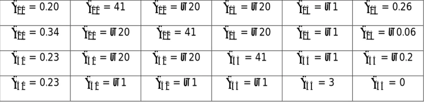
= ∙ (H.18) = + ∙ + ∙ + ∙ + ∙ (H.19A) = + ∙ + ∙ + ∙ + ∙ (H.20) = + ∙ + ∙ + ∙ + ∙ (H.21A) ∙ = + ∙ + ∙ + ∙ + ∙ (H.22)

Now, we arrive to the second stage of Keynes’s (1936, 166) decision-making process in which households decide how they allocate their wealth. Demand for various assets is depicted in the portfolio equations above following Tobinesque principles. Adding-up constraints, emphasized by Tobin (1969), are satisfied.

The demand for cash is a fraction of consumption as in Godley and Lavoie’s (2012) model INSOUT (H.18). The underlying idea is that households conduct a certain amount of their

47

consumption transactions with cash and its demand does not depend on the rates of return on other assets.

The fraction of demand deposits to expected wealth net of cash depends positively (the coefficient is positive) on an autonomous and a transaction term (first and last term on the right-hand side) and negatively on rates of return on other assets (H.19A). In turn, the fraction of time deposits depends positively on an autonomous term and its own rate of return (first two terms on the right-hand side) and negatively on rates of return on other assets and transactions (H.20). Similarly to time deposits, the fraction of bills depends positively on an autonomous term and its own rate of return and negatively on rates of return on other assets and transactions (H.21A). As with time deposits and bills, the fraction of bonds also depends positively on an autonomous term and its own rate of return and negatively on rates of return on other assets and transactions (H.22).

48

A

PPENDIX

:

L

IST

OF

V

ARIABLES

[InsertTable3]

[InsertTable4]

[InsertTable5]

49

F

OOTNOTES

1 _{For a detailed discussion on the similarities and differences of various FRB versions see} Anonymous (2015a).

2 _{A previous version of the model called REFORM was published in Anonymous (2015b).}

4_{The market value of government debt can differ from its recorded historical value, which is} generally reported by officials, to the extent that bond prices have appreciated or depreciated. However, as the bond rate is set exogenously, there cannot be any changes in bond prices and, thus, in this instance the market value of government debt also equals its recorded historical value.

8 _{In the model INSOUT bills are also held by banks. This – in addition to the fact that households} can directly decide in which form they want to hold government debt and not only as a result of reallocation – explains why households do not buy as many bills under endogenous money than under FRB without money creation.

9_{To analyze the effects of creating new money through citizen’s dividend some equations have} been modified. Citizen’s dividend has been added as an additional source of funds to regular disposable income of households (H.1). Similarly, citizen’s dividend is added as an additional expenditure for the government (G.2).

50

Table 1. Balance sheet matrix

Households Firms Government Central bank Banks Sum

Inventories +IN +IN

Cash and reserves +Hh −Hs +Hb 0

Demand deposits +M1 −M1 0 Time deposits +M2 −M2 0 Bills +Bh −Bs +Bcb 0 Bonds +pbL·BL −pbL·BL 0 Loans −L +L 0 Balance −V 0 +GD 0 0 −IN Sum 0 0 0 0 0 0

52

Table 2. Transaction-flow matrix

Households Government Sum

Current Capital Current Capital Current Capital

Consumption −C +C 0

Government expenditures +G −G 0

Change in inventories +∆IN −∆IN 0

[Memo: GDP] [Y] [Y]

Sales tax −T +T 0

Wages +WB −WB 0

Entrepreneurial profits +Ff −Ff 0

Bank profits +Fb −Fb 0

Central bank profits +Fcb −Fcb 0

Interest on loans −rl -1·L-1 +rl-1·L-1 0

…time deposits +rm-1·M2-1 −rm-1·M2-1 0

...bills +rb-1·Bh-1 −rb-1·Bs-1 +rb-1·Bcb-1 0

...bonds +BL-1 −BL-1 0

Change in the stock of loans +∆L −∆L 0

…cash and reserves −∆Hh +∆Hs −∆Hb 0

…demand deposits −∆M1 +∆M1 0

…time deposits −∆M2 +∆M2 0

...bills −∆Bh +∆Bs −∆Bcb 0

...bonds −pbL·∆BL +pbL·∆BL 0

Sum 0 0 0 0 0 0 0 0 0

Note: Plus signs indicate sources of funds and minus signs uses of funds.

53

Table 3. List of Endogenous Variables

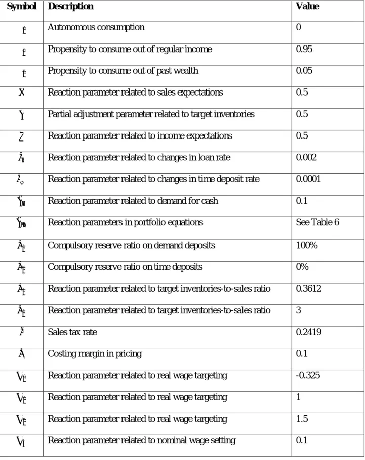
Symbol Description Initial value

Bills held by central bank 50

Bills demanded by households 29.02

Bills held by households 29.02

Bills supplied by government 79.02

Bonds demanded by households 1.29

Bonds held by households 1.29

Bonds supplied by government 1.29

Bank liquidity ratio 1.14

Bank profit margin 0.0032

Real consumption 108.87

Nominal consumption 178.99

Capital gains 0

Total profits distributed to households 16.40

Profits of banks 0.27

Profits of central bank 0.39

Entrepreneurial profits 16.13

Expected entrepreneurial profits 16.13

Nominal government expenditures 41.39

Gross government debt 126.80

Consolidated government debt 76.80

Reserves held by banks 32.09

54

Cash held by households 17.9

Reserves required from banks 28.02

Cash and reserves supplied by central bank 50

Real inventories 43.54

Real short-term target inventories 43.54

Real long-term target inventories 43.54

Nominal inventories 52.2

Loans demanded by firms 52.2

Loans supplied by banks 52.2

1 Demand deposits demanded by households 28.02

1 Demand deposits held by households 28.02

1 Demand deposits supplied by banks 28.02

2 Time deposits demanded by households 56.27

2 Time deposits held by households 56.27

2 Time deposits supplied by banks 56.27

Employment level 134.05

Normal historic unit costs 1.203

Price level 1.64

Price of bonds 37.03

Public sector borrowing requirement (government budget deficit) -0.01

Interest rate on bills 0.80%

Interest rate on loans 1.2%

Interest rate on time deposits 0.64%