Technical trading with open interest:
evidence from the German market
• Thorben Manfred Lubnau
Department of Business Administration,
in particular Finance and Capital Market Theory European University Viadrina
Große Scharrnstraße 59 D-15230 Frankfurt (Oder) Germany
E-mail: lubnau@europa-uni.de
• Neda Todorova, corresponding author
Department of Business Administration,
in particular Finance and Capital Market Theory European University Viadrina
Große Scharrnstraße 59 D-15230 Frankfurt (Oder) Germany
E-mail: todorova@europa-uni.de
This article investigates whether options’ open interest can be incorporated suc-cessfully into technical trading strategies. A set of 2040 trading rules is applied to the German index DAX 30 and to the ten German stocks with the highest market capitalization. The results show that open interest rules, when combined with infor-mation from the spot market, can improve the predictive power of technical trading rules. Both put and call open interest appear to contain information regarding future equity prices while the open interest differential performs very poorly. Best results are achieved for the DAX index, showing economically significant profits even when transaction costs are taken into account whereas the results are more mixed for individual options. Across all assets, out-of-the-money calls and in-the-money puts exhibit the strongest forecasting power for the utilized rules.
I. Introduction
Technical analysis may be defined as a variety of methods that aim at forecasting the movements of prices of financial instruments by extracting information from his-torical data. Technical analysts try to identify trends at an early stage and maintain their positions until a trend reversal is signalled. This article links technical analy-sis to options market activity and investigates whether traders who use information contained by options markets are better off than traders who do not. Specifically, we investigate the German equity market by deriving trading signals from the spot market and the open interest of options.
The discussion among academics and practitioners about the merits of technical analysis has been ongoing over decades. As pointed out by Taylor and Allen (1992) and Menkhoff and Taylor (2007), technical rules are widespread amongst practition-ers, for example in the foreign exchange market. However, technical analysis has been the black sheep in financial economics as it is not built on solid theoretical foundations but is rather a set of ad-hoc rules. Neftci (1991) calls it ”a broad class of prediction rules with unknown statistical properties, developed by practitioners without reference to any formalism”, and Malkiel (2003) an ”anathema to the aca-demic world”, as it contradicts one of the main foundations of modern finance, the Efficient Market Hypothesis (EMH), proposed by Fama (1970). The EMH states that prices on efficient capital markets fully reflect all information and will adjust immediately to new information. Fama (1970) proposed an additional subdivision of the EMH into three forms of efficiency: The weak form, in which the informa-tion set contains only historical capital market data, the semi strong form, in which the information set comprises all public available information, and the strong form, in which the information set contains all available information. Therefore, if price trends could be exploited profitably by means of technical analysis, capital markets are not even efficient in the weak form.
of studies have researched the performance of technical trading rules. A concise overview on the topic is given by Park and Irwin (2007). Most researchers in the field of technical trading rules (e. g. Brock et al., 1992; Bessembinder and Chan, 1998) focus on historic prices in the spot market without searching for other po-tential sources of information like the derivatives market. Options are redundant securities in a complete, Black-Scholes market. In real world settings, however, if the options market attracts informed traders, option transactions may first reflect in-formation which has not been incorporated in the spot market yet. The asymmetry of information and the preference for trading in derivatives would thus cause op-tion trading activity to reveal informaop-tion about future changes in stock and opop-tion prices. Stephan and Whaley (1990) note that because the options market offers low transaction costs and high financial leverage, both liquidity and informed traders will be attracted to it. Furthermore, trading in options may overcome possible short sale restrictions. Cao (1999) shows within theoretical settings that increased trad-ing opportunities due to derivatives create an incentive for traders to collect private information about asset payoffs.
In early studies, Manaster and Rendleman (1982), Bhattacharya (1987) and An-thony (1988) find that the options market actually leads the spot market. Stephan and Whaley (1990), by contrast, find stocks to lead their options in terms of both intraday price changes and trading activity. A large body of following literature examines the price discovery relations between the spot and options market empir-ically, mostly focusing on options trading volume. Examples include but are not limited to Vijh (1990), Mayhew et al. (1995), Kumar et al. (1998), Chan et al.
(2002), Chakravarty et al. (2004) and Pan and Poteshman (2006). Their findings confirm that options are not redundant in explaining the returns of risky assets and can actually lead the spot market. A theoretical treatment of the lead-lag relation between option and spot markets is provided by Easley et al. (1998) who assume that the decision of informed traders to participate in the option market arises
endogenously within an equilibrium framework. They show that under plausible assumptions informed investors would actually trade in the option rather than the spot market so that option transactions should contain valuable information about future prices.
Regarding the profitability of trading rules, fewer researchers study the informa-tional content of options markets. Most of these studies focus on specific trading strategies based on the options’ implied volatilities and examine trading in options and not in the underlying asset (e.g. Bluhm and Yu, 2000; Jha and Kalimipalli, 2010). Goyal and Saretto (2009) for instance refer to the mean-reverting feature of stock volatility and show that trading strategies based on sorting stocks according to the difference between historical realized volatility and implied volatility generates statistically significant returns. Applying classical technical trading rules to options open interest is considered, to our knowledge, only in the study of Charlebois and Sapp (2007). They report that the differential of call and put options open inter-est has the potential to generate significant excess returns in the foreign exchange market.
This article contributes to the existing literature in two ways. First, the study of Charlebois and Sapp (2007) is extended to the equity market. Recognizing the po-tential concerns of data snooping regarding the results of technical trading rules, we do not concentrate on one asset only but investigate eleven securities. Specifically, we apply a uniform set of 2040 trading rules to the German index DAX 30 and to the ten stocks with the highest market capitalization on the German market. The only requirement for the selection of the stocks is the availability of open interest data for the whole period under consideration. The sample is hence characterized by a material diversity in terms of total return and return variability. The data set extends from January 2000 to June 2010 and contains only free of cost publicly available data. To assess the significance of the attained results, standard boot-strapping methods are applied. The profitability of the trading rules is evaluated
by establishing break-even transaction costs.
Second, this study comprises a thorough investigation of options’ open interest. Following Charlebois and Sapp (2007), we first explore the differential between calls and puts open interest and find no evidence that it can forecast temporal patterns within the utilized rules. A crucial point for explaining the different results may be the nature of the explored markets. Possibly, hedging activities are predominant on the forex market. In the stock market there might be a clear informational advan-tage regarding important corporate announcements for certain market participants as collecting private information appears to be much simpler for a single equity. In-ferring information from the open interest distribution across the options moneyness, we suppose that some market participants actually possess private information and trade on it. Noting that informed traders can establish bullish positions with puts as well as calls, an increase of the put open interest does not necessarily indicate a market expectation of falling prices. Besides investigating the patterns in the open interest differential, we therefore analyze the open interest behaviour of put and call options separately.
A major finding of the article is that both put and call open interest exhibit forecasting power for establishing profitable trading strategies although they fail to beat a very simple moving average strategy profitwise. The technical trading rules perform by far the best for the DAX index, generating economically significant profits even after trading costs. Results for the individual stocks are more mixed but indicate that open interest may be an useful indicator of future market movements and it is reasonable to incorporate it in technical analysis based on historical prices. Considering different moneyness ranges, out-of-the-money calls and in-the-money puts have the highest potential to generate correct trading signals with the used rules, which is a intriguing result about the trading activity on the Eurex.
The article is arranged as follows. Section II outlines the motivation for the inves-tigated trading strategies based on open interest. Section III presents our
method-ology. Section IV discusses the data sets we use. Results are given in Section V. Section VI concludes.
II. Option markets and open interest
Open interest has been an acknowledged important indicator for future price pat-terns among practitioners but is subject of limited research in the financial literature, as compared to option volume. The informational role and forecasting power of open interest is investigated by Donders et al.(2000), Jayarmanet al.(2001), Yanget al.
(2001), Bhuyan and Chaudhury (2005) and Bhuyan and Williams (2005), among others. These studies suggest that open interest is likely to be informative about the future movements of the stock prices and the behaviour of derivatives markets participants as a whole. Compared to trading volume, open interest offers a crucial advantage. Although trading volume in derivatives markets may contain informa-tion regarding the price discovery process in spot markets, volume itself gives no indication about the direction of the transactions. In extreme cases for example, the whole daily transaction volume may be attributed to closing positions. For this reason, open interest in options markets may provide additional insights in regard to the informational role of options.1
Charlebois and Sapp (2007) investigate whether the differential between the num-ber of outstanding call contracts and outstanding put contracts may be informative for the foreign exchange market and find that strategies using information from at-the-money options are more profitable than the common strategies based solely on historical spot exchange rates. Their approach is motivated by the idea that informed investors would be better off taking long positions in option contracts that match their views. Consequently, an increasing (decreasing) differential between call and put options outstanding is to be interpreted as a bullish (bearish) signal.
The examination of possible option strategies shows that the impact of bullish
strategies on open interest is not necessarily that clear. For example, Easley et al.
(1998) discern between positive and negative option volume. Trades that arise from positive news are buying a call or selling a put. Accordingly, negative news provoke buying a put or selling a call. Caoet al.(1999) and Jayarmanet al.(2001) summarize simple bullish strategies for an informed trader. These may contain purchasing a call option, shorting a put option, purchasing the stock and shorting a call option, closing a previous short call position, closing a previous long put position, establishing a bullish call, bullish put or bullish calendar spread. Such strategies can either increase or decrease the open interest. Since informed traders can employ puts as well as calls as a reaction to a bullish expectation, we argue that an enhanced differential between call and put open interest is not necessarily a sign of rising spot prices. It seems more appropriate to analyze the open interest behaviour of put and call options separately.
In a comprehensive study on the US market, Lakonishok et al. (2007) present surprising results about the trading activity on the CBOE over the period from 1990 to 2001. Among purchased puts and calls, purchased puts appear to be the least common. So, written put open interest prevails over purchased put open interest. Furthermore, Jayarman et al. (2001) show that around merger announce-ments informed traders prefer higher leveraged, shorter-term options and besides the amount of call contracts outstanding, the open interest of put contracts also rises significantly. Their data comprise a large sample of companies with option trades on CBOE from 1986 to 1996. Similar results are reported by Donders et al.(2000) for earnings announcements over the period 1991 to 1993 for assets with options traded on the AEX Options Exchange, indicating that informed traders could prefer put options to profit from private information. Motivated by these research results, we interpret the increase of puts open interest as a bullish signal. To sum up, for identifying profitable trading rules employing open interest, we study whether an increase (decrease) of open interest of call contracts, put contracts or open interest
differential may confirm an upward (downward) trend.
III. Methodology
Trading RulesThe term technical analysis subsumes literally hundreds of different rules based on the evaluation of historic price data, trading volume and open interest. A well known set of technical rules is made up of moving averages (MA) of different lengths. Menkhoff and Taylor (2007) classify MA as quantitative form of technical analysis, in contrast to qualitative forms of chart reading that rely on a more subjective as-sessment of the analyst. Signals are generated whenever the shorter moving average crosses the longer moving average. This system may be considered to be one of the most basic in technical analysis as, when the trader has decided which lengths to use, no further human input is necessary to keep the system going. The possibility to evaluate automated trading system has made moving averages so appealing to researchers. Following the seminal article by Brock et al. (1992), who used moving averages and trading range break-out systems, numerous studies tested the predic-tive power of such systems in various markets (see for example Hudson et al., 1996; Bessembinder and Chan, 1998; Coutts and Cheung, 2000; Wong et al., 2003).
Usually the moving averages are calculated for price series. Information on historic stock prices is in almost all cases readily available. The computational effort is manageable as even spreadsheets allow the calculation of moving averages. The rules of our simple MA system are as follows. The short moving average (SM A) is
SM At= 1 n n−1 X i=0 St−i (1)
For the Long Moving Average we have LM At= 1 m m−1 X i=0 St−i (2)
A Buy signal is generated when the SM A crosses the LM A from below. Con-versely, a Sell signal is generated when theSM Afalls below theLM A. However, we extend the simple moving average of spot prices by combining it with open interest from the option market and by testing the predictive power of a moving average system of open interest series. The latter consists of the rules 1 and 2 and the signal generating algorithm described above. We only substitute the spot prices with the relevant open interest data sets.
The combined system of spot and open interest moving averages divides the sam-ple period into Buy days, Sell days and Neutral days. Whenever the moving average rules of both the spot price series and the open interest series show that a Buy (Sell) signal is in effect, we classify this day as a Buy (Sell) day in the combined system. Opposed to the simple MAs described above, it is now possible that we receive contradictory signals from the spot and the options market, meaning that one MA points to a Buy and the other to a Sell day. In this case, we classify this day to be a Neutral day.
There is no universal rule how to chose m and n. Charlebois and Sapp (2007) use n = {1,2,5,10} and m = {25,50,75,100}. However, in Brock et al. (1992),
n = 1 and m = 200 is referred to as the most popular moving average rule and is tested as well as m = {50,150}. To provide a rather complete survey we use a mixture of the rules employed by Charlebois and Sapp (2007) and Brock et al.
(1992) by setting n = {1,2,5,10} for the simple moving average systems and n =
{1,5} for the combined rules. Incorporating the rules of Brock et al. (1992) we set
m={25,50,75,100,150,200}. So, to summarize, we test open interest differentials as well as puts and calls separately. These three categories are considered for all
options and subsets divided into moneyness ranges. All subsets of open interest data are evaluated on standalone basis and also combined with the spot rules. Therefore, we test a total of 2040 rules for each asset.
Trading Systems
After the Buy and Sell signals are generated an investor has to decide on which strategy to implement. An obvious choice would be to hold the stock or index on Buy days and to move out of the market on Sell days, probably investing in money market instruments.
We, however, consider a different strategy than the one described above as it would not take full advantage of successful technical rules. We implement a Long and Short strategy (LS) where we hold the stock or index on Buy days, short it on Sell days and move into the money market on Neutral days. Obviously, LS is advantageous when the rules are able to identify periods of falling prices. Taking a closer look at returns for the LS, the investor earns the stock’s or index’s return rs
on Buy days. On Neutral days LS earns the risk free raterf. Consequently, on Sell
days LS earns −rs. Bootstrap
To evaluate the statistical significance of our results, we employ the bootstrap methodology as described in Efron and Tibshirani (1986). This statistical method was introduced by Brock et al. (1992) to the field of technical analysis of stock markets and is widely used to assess the power of automated trading rules (Bessem-binder and Chan, 1998; Kwon and Kish, 2002; Charlebois and Sapp, 2007; Levich and Thomas, 1993 for the foreign exchange market). From our point of view, the bootstrap is better suited than an ordinary t-test as the latter poses strict assump-tions on the data tested. It is questionable whether stock returns are normally distributed and possess homoscedastic variance. Furthermore, as we compare re-turn series derived by certain rules from all rere-turns observed, the series may not be independent.
We use a random walk model to perform the bootstrap test for the spot rules. From the original time series, daily returns are randomly drawn with replacement and then a new price series is constructed according to
log St∗+1
= log (St∗) +rt∗+1 (3)
Each new series starts with the natural logarithm of the observed initial price,
S0∗ = S0. For every asset 1000 bootstrap samples are created according to the
rules described above. The technical trading rules are then applied to each of those samples.
To generate bootstrap samples for the open interest series, we resample the daily differences by drawing with replacement from the observed time series. As for the prices we create new open interest histories by starting with the observed initial value and then adding randomly drawn increments.
As in Efron and Tibshirani (1993), the approximated achieved significance level for every statistic of interest (for example mean returns on Buy and Sell days, standard deviations) is given by
[
ASL= #{t(S
∗i)≥t(S)}
B , i= 1, . . . , B, B = 1000 (4)
This means we are counting the number of bootstrap samples showing a larger value for the computed statistic than the original series. This number is divided by
B, the total number of bootstrap samples performed. The resulting approximate significance level can be interpreted as a simulated p-value.
We consider the difference between mean returns on days where a buy signal is in effect (Buy days) and days where a sell signal is in effect (Sell days) to be an appropriate measure of the predictive power of a technical trading system. This is because a significant difference means that the system is able to distinguish between days with a higher return and those with a lower (hopefully negative) return.
Another point of interest is the evaluation of the standard deviation on Buy and Sell days. Previous studies showed that the standard deviation on Buy days tends to be lower than on Sell days. It is also lower than the unconditional standard deviation of a buy and hold strategy. This may be due to the leverage effect, which states that as stock prices fall there is an increase in the debt-equity ratio of a company and investors perceive the stock to be more risky.
Transaction Costs
When evaluating the performance of technical trading systems a crucial point to consider are transaction costs. Way too often investors overlook the fact that just because a trading system is able to predict market trends correctly it does not guarantee economic profits. However, whether one will finally end up with a profit does depend on the number of signals the system generates.
Following the methodology set out in Bessembinder and Chan (1998) we calculate break-even transaction costs. Every Buy or Sell signal leads to a change of 200 % of the investor’s equity position. This can be seen by taking the example of a Buy signal. Let us assume that the investor starts with a neutral position in the LS-system. After observing the Buy signal he shifts his money from the money market to the stock market. This equals 100 % of his initial equity. When the buy signal is no longer in effect, whether because there are contradictory signals or a Sell signal, the position is reversed to neutral. This is again a shift of 100 % back to the neutral position.
To calculate the break-even transaction costs, we therefore count the Buy and Sell signals. To evaluate whether the investor is better off with the trading system or with a buy and hold strategy, we calculate the excess return of the trading rules against buy and hold. Let rex be the excess return, then the break-even transaction
costs T C are calculated as follows,
TC = rex
IV. Data
We use daily closing prices of the German blue-chip index DAX 30 and ten DAX components from XETRA as well as dividend data of these equities. Since the DAX 30 is a performance index, it is not necessary to consider dividend yields for performing technical trading on it. Furthermore, open interest data for the index and stock options traded on the Eurex are considered. As a proxy for the money market interest rates we use the one-month Euribor. The data include the period from January 3, 2000 up to June 30, 2010 for a total of 2667 trading days. The option data from 2000 to 2006 were supplied to us by the Eurex. All other data were obtained from Datastream.
The stock sample consists of the ten companies with the highest market capi-talization as of August 1, 2010.2 The stocks give wide market coverage in terms
of sector representation. Allianz (ALV) and Deutsche Bank (DBK) belong to the financial services sector. The chemical stocks are Bayer (BAY) and BASF (BAS). Volkswagen (VOW) and Daimler (DAI) represent the manufacturing industry. SAP and Siemens (SIE) are technology stocks. RWE is an utilities provider and Deutsche Telekom (DTE) is a telecom stock.
The stocks’ closing prices are first adjusted to stock splits (SAP, 2000 and 2008, BASF 2006) in a prospective manner. Subsequently, spot prices are adjusted, also prospectively, by multiplying them with a dividend adjustment factor. After the first dividend adjustment, this factor amounts to
FAdj = S Ex U nadj+D SEx U nadj (6) where SEX
U nadj is the unadjusted closing spot price after the payment of dividend D.
As the sample period covers multiple dividend payments, updates of the adjustment factor are necessary. The relevant adjustment factor after each subsequent dividend
2E.ON is excluded from the sample as the corresponding stock options are not available for the
payment is obtained by multiplying the extant factor with the new one, which is again computed using equation 6. This procedure ensures that dividend payments do not trigger trading signals within the historical moving averages rules due to sudden drops of the spot price. Furthermore, it guarantees that dividends are taken into account when measuring the returns of the trading strategies.
Table 1 reports key characteristics of the investigated assets. To give some sense of the magnitude of volatility associated with a given asset, the coefficient of variation is reported. It is clearly seen that the sample covers assets with very different characteristics in terms of total return and price variation over time.
Besides the spot market data, we utilize an important source of information from the option market, the open interest. The open interest indicates the number of option contracts outstanding at the end of a given day. The data set comprises the daily amounts of outstanding puts and call option contracts for the existing maturities and strike prices. Because of compiling the data, open interest data is published at 1:30 pm for the previous day on the Eurex website. The data sample from Eurex takes this lag into account. Datastream attributes the corresponding value to the previous day. To establish comparability between both data sources, we lag the Datastream open interest by one trading day. So, as we use open interest data publicly available at the middle of the day to trade in the underlying asset at the end of the same trading day, our results are not vulnerable to nonsynchronicity bias as known from other studies of technical trading.
Since the option interest data from 2000 to 2006 is from Eurex whereas the rest of the sample period is based on Datastream, an important concern is a potential bias arising from the utilization of different data bases. For the time period from January 2006 to September 2006, data from both sources are available. Given this data overlap, we randomly compared pairwise the time series of various individual options to insure conformance. This check did not yield any indications of disparity between the data sources. Therefore, no notable bias is expected to distort the
results of the study.
Only European DAX index options are traded on the Eurex. On the contrary, all equity options are American-style. As the early exercise of American options reduces open interest, dividend payments may generally have a distorting impact on the trading strategies. However, many researchers (e.g. Diz and Finucane, 1991; Poteshman and Serbin, 2003; Haoet al., 2010) provide evidence that option holders often seem to follow a suboptimal exercise policy. Because a thorough investigation of the open interest behaviour around dividend payment days did not identify a consistent strong reduction of the existent open options’ positions, we disregard a special treatment of the dividend days.
We restrict our analysis to options with a time to maturity greater than 15 cal-endar days and less than 90 calcal-endar days as these are the most actively traded options in our sample. We impose a minimum of 15 calendar days to maturity to avoid distorting signals caused by the nearing options maturity. Our results are, however, similar if we allow very short-term options or longer-term options to be included.
Moneyness is defined as the ratio between the price of the underlying asset and the strike price for calls, and the reciprocal value for puts, respectively. As the options in each moneyness category exhibit different properties, they may contain different information so we consider them also separately. For example, at-the-money (ATM) options are often the most liquid so investors may prefer to employ options of this category. On the other hand, deep out-of-the-money (OTM) options offer the highest leverage so informed traders could prefer these contracts. As traders possessing private information would benefit mostly from leveraging their position using OTM options, researchers often concentrate on the informational role of OTM options (e.g. Bates, 1991). This is particularly relevant for stocks, where informed traders may have an obvious informational advantage regarding important corporate events.
Table 2 disaggregates the average daily open interest by moneyness. The options are split into five categories ranging from deep in-the-money (ITM) options (category 1) to deep OTM options (category 5). We compute the moneyness of the option data by referring the strike prices to the unadjusted spot prices of the underlying assets as the Eurex conducts no adjustments of strike prices of existent options due to ordinary dividend payments. For purposes of comparison, it is important to take into account that all equity options have a contract size of 100 shares except ALV (10) and SAP (50).
A number of interesting observations about the distribution of open interest across the moneyness ranges can be made. It is a stylized fact about open interest that a plot of dependence for calls and puts shows a peak near the ATM contracts (see Buraschi and Jiltsov, 2006; Lakonishok et al., 2007). This feature seems to be inde-pendent of the underlying asset and options maturity for many markets. However, Judd and Leisen (2010) show that in incomplete markets under specific theoretical assumptions about investors’ utility functions, the shape of the open interest curve is very sensitive to the number of options traded, to the type of distribution and the location of the strike grid and thus can contradict the aforementioned stylized fact. Table 2 provides evidence that departures from the common distribution of the open interest over strike prices occur on the Eurex. The expected peak for near-the-money contracts can be observed only for the calls on DAX, BAS, RWE and SAP and the puts on DTE. For almost all assets the biggest part of open con-tracts is deep out-of-the-money. This is actually a striking observation. A possible explanation is that a substantial part of the trading activity on the Eurex market is guided by private information or follows speculative purposes such that investors employ OTM options to leverage their positions.
Furthermore, we observe that in most cases there are more open positions in deep ITM options than in options that are slightly ITM. Overall, it is possible that market participants have a tendency to open option positions near the money as observed by
Lakonishoket al. (2007), but their options holdings become less concentrated near-the-money when the underlying prices move away from the original strike prices. This is relevant especially for highly volatile securities.
Lastly, the open interest shows a high variation over time across all moneyness ranges. This may be due to the expiration of the most liquid contracts in March, June, September and December. In the following, we will report whether large changes of open interest may provide information about future spot prices despite of this seasonality.
V. Results
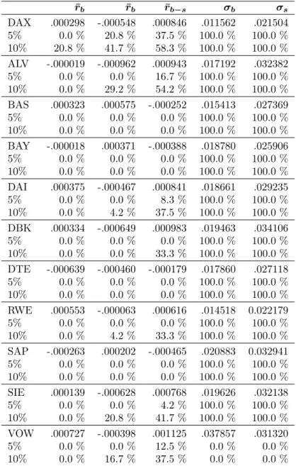
Spot rulesThe results for the trading rules based on historical spot prices are given in table 3. Results for mean Buy and Sell returns across the relevant trading rules are displayed in the columns labelled as r¯b and r¯s. r¯b−s denotes the average difference of returns
on Buy and Sell days. The mean values of the standard deviations are presented in the columns labelled σb and σs. The statistical significance of the results from
each rule is assessed using a bootstrapping methodology with 1000 samples. The percentages below each value of mean returns and standard deviations denote how many of the rules achieved significance according to the simulated p-values at the 5 % and 10 % level, respectively.
The results for popular technical trading rules based on historical prices indicate that moving averages have some forecasting power, which, however, varies substan-tially across assets. The forecasting ability is most pronounced for the DAX. 37.5 % (58.3 %) of the rules applied to the index lead to mean differences of returns on Buy and Sell days significant at the 5 % (10 %) level. Furthermore, six stocks achieve significant values forr¯b−sat the 10 % level with more than 30 % of the explored rules
The remaining four stocks (BAS, BAY, DTE and SAP) exhibit negative values for r¯b−s and without exception achieve no significantly positive differences between
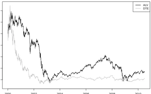
mean Buy and Sell returns. An analysis of the stocks’ price patterns may shed light on the possible reasons for this bad performance. SAP and BAY have the lowest price variation among all considered assets (see table 1). It is generally harder to generate profits from timing an asset without distinct price trends. This is also obvious in the case of DTE: DTE has the lowest total return (-78.04 %), with a sharp price decline of almost 80 % during the first one and a half years of the sample. This price deterioration is followed by years without strong trends. Such a price pattern offers very restricted potential for generating positive Buy returns. For comparison, ALV is characterized by a total return of a similar magnitude (-66.68 %) but shows clear upward and downward periods over the whole sample period. As a matter of fact, for ALV the spot trading rules generate an average negative return. On Sell days, however, mean returns are much lower so that the spot rules manage to beat significantly the buy and hold strategy in 54.2 % of the cases. Fig. 1 shows the price history of both stocks over the period under consideration.
Finally, the poor performance of BAS is surprising as this stock has the highest total return of 170.41 % and a comparatively high variation of the daily price obser-vations. Probably, the inability of technical analysis to capture temporal patterns is due to the fact that over the first five years, the price has a very smooth course. It is a very challenging venture to beat the simple buy and hold strategy in such a context. This observation indicates the necessity of technical trading in separate stocks using only spot rules to be accompanied by fundamental corporate analysis. It is also noteworthy that the standard deviations of the Buy periods for spot rules are significantly lower than those of the Sell periods. Obviously, the trading rules are able to identify periods of low volatility with Buy signals. This is consistent with the results of Brock et al. (1992). The only exception is VOW, implying that the positive excess returns may be interpreted as a compensation for bearing risk.
20 40 60 80 100 120 140 03/01/2000 = 100 2000 2002 2004 2006 2008 2010 ALV DTE
Fig. 1. ALV and DTE stock prices 01/2000 - 06/2010, 03/01/2000 = 100
Open interest and combined rules
Results from trading rules based on open interest (OI rules) are presented in table 4. We distinguish between the results for rules applied to call and put open interest as well as to the open interest differential. A surprising finding is that open interest differential performs worst across all securities. Using solely this source of information does not generate notable and significantly positive Buy-Sell differences. Combining the open interest differential and the spot rules is not able to improve the performance. Exceptions are ALV, SIE and VOW, for which about 45 % to 55 % of the combined rules yield significantly positive values for rb¯−s at the 10 % level.
This strikingly weak performance of the open interest differential is opposite to the findings of Charlebois and Sapp (2007). They argue that using the open interest differential instead of the number of puts or calls positions separately avoids false trading signals triggered by the expiration of options contracts and thus is able to yield more stable results. Obviously, the intuition that an increase in the open interest differential is to be interpreted as a bullish signal is too simplifying for the
Eurex market.
Regarding puts and calls separately, technical trading performs much better for the DAX index than for the equities. This is consistent with the results of the spot rules. Both calls and puts have a pronounced forecasting power with puts being a more powerful predictor. In the case of puts, incorporating both open interest and spot information in the trading strategies generates average Buy-Sell differences which are significant at the 5 % (10 %) level for 97.22 % (100 %) of the explored rules. This result confirms that the market participants react to bullish signals by employing strategies with both puts and calls options. However, the forecasting power of open interest of the DAX index contradicts the findings of Booth
et al. (1999) who investigate the price discovery process of the index DAX and its futures and options contracts using a multivariate vector error correction model and present evidence that the spot index and index futures exhibit considerably larger information shares than index options. The sample period of their study contains much older data (January 1992 to March 1994) when option markets in Germany supposedly played a minor role compared to later years. Furthermore, the study of Booth et al. (1999) is based purely on price relationships and does not take open interest into account.
For all stocks, the open interest rules with calls and puts and the corresponding combined rules generate positive mean differences of returns on Buy and Sell days. It is to be distinguished whether the spot rules for the given stock have exhibited predictive power. For the four equities with weak performance of the spot rules, the OI rules result in positive average returns on Buy days. Utilization of open interest information has obvious forecasting power, especially for BAS and DTE, but com-bining open interest with spot market signals leads to a deteriorating performance, as expected. For the remaining six equities, the OI rules with puts and calls result in higher average returns on Buy days than the spot rules in almost all cases. Em-ploying both the spot and derivatives market as sources of information consistently
improves the results so that much more that 50 % of the combined rules yield sig-nificantly positive Buy-Sell differences. The superiority of puts contracts is obvious for all stocks. Puts perform weaker in terms of the number of rules with significant results only for DTE and SAP from the stocks with poor spot rules’ performance, and for ALV.
This somewhat stronger predictive power of puts may be explained by the results of Lakonishok et al. (2007) which establish that “purchased put open interest is smaller than written put open interest and smaller still relative to both purchased and written call open interest”. Since market participants pursue different expecta-tions when purchasing or writting opexpecta-tions, the forecasting power of purchased and written calls supposedly offsets each other whereas the forecasting power of written put open interest might outweigh the distortion caused by purchased put open in-terest. Moreover, our trading rules for put open interest are appropriate exactly for capturing bullish signals from written puts.
An intriguing observation for rules based solely on open interest is that the stan-dard deviations of the Buy periods are significantly higher than those of the Sell periods across all assets and data sets. The fact that higher returns for Buy days are generated during more volatile periods indicates that trading solely on open interest may comprise substantial risks. Combining information from spot and op-tions market consistently reverses the proportion such that following a Buy signal the volatility is significantly below the volatility after sell signals.
Moneyness ranges
After identifying that consideration of open interest adds value when investing in the underlying asset, it is to be investigated whether forecasting power may be attributed to a specific moneyness range. Table 5 reports results for the open interest and combined rules applied separately for ITM, ATM and OTM options. For brevity, only the percentages of bootstrap samples with inferior results at the
10 % level are presented.3
Regarding calls’ open interest, the best results are achieved with OTM options in most cases. This is in line with the expectation that OTM options are attractive for informed investors. OTM options are generally less liquid and thus have higher rel-ative bid-ask spreads than ATM and ITM options. But, in the presence of superior information, the leverage effect may dominate the liquidity consideration. Consis-tent with our previous results, the performance of the combined rules deteriorates for the stocks with poor spot rules’ results and improves for the remaining assets.
In the case of puts, it can be discerned that ITM puts are often superior to the other moneyness ranges. At first glance, this is a surprising observation, especially in the context of the observed investors’ preference for OTM calls. Probably, the results for OTM puts may be improved by imposing Buy signals for falling open interest, contradictory to our rules. On the other hand, shorting ITM puts prior to price increases offers clear advantages as options with lower strikes provide higher option premiums. Furthermore, the ITM range may allow informed investors to hide their trades better. Our results about the relative superiority of ITM puts are in conformity with Lakonishoket al. (2007) who indicate, as noted above, that written put option interest is much higher than purchased put option interest.
Particularly noteworthy is also the much better performance of the technical strategies applied to the stock index compared to the individual stocks. For all moneyness ranges of the DAX, the trading rules lead to a very high number of sta-tistically significant excess returns. Again, OTM calls and ITM puts yield the best results.
Lastly, there is still conclusive evidence that the combined trading strategies dis-tinguish between days of high and low volatility and Sell signals are mostly attributed to the latter.
Transaction Costs
3Detailed results for the returns and standard deviations across all rules, assets and moneyness
The average break-even transaction costs for all tested rules, divided by utilized source of information and moneyness, are reported in table 6. Our results are quite mixed. For the DAX and six out of the ten stocks analysed, our trading rules are able to generate excess returns over a buy and hold strategy that seem to be large enough to leave an investor with some profit after deducting transaction costs. We assume that break even costs of 0.5 % are large enough to make the implementation of a trading system profitable. Today, even private investors can trade at costs below this threshold at various online brokers.
Of the systems tested, the standalone spot rules fare the best concerning break-even costs. This is due to the fact that they generate the lowest number of trading signals of all systems. For the DAX, ALV, DBK, SIE and VOW we calculate break-even costs in excess of 1 %, with those for ALV being over 2 %. DAI is just below 1 % and DTE at about 0.9 %. For the four other stocks, break-even costs are negative or only slightly positive.
The combined systems generate lower profits due to the rising number of trans-actions that is not offset by higher returns. However, when all options are used to generate signals, the aforementioned assets have break-even costs above 0.5 %. It is an interesting fact that results are worst when we use the open interest differential as input. This confirms our previous results for the poor predictive power of the open interest differential. Puts and calls are more profitable.
Using only open interest without the price moving averages yields results below the simple moving average system and the combined rules. It may be questioned whether they generate economically significant profits. As for the combined rules, we find that the open interest differential cannot keep up with the puts and calls.
Overall, it must be pointed out that disaggregating into moneyness ranges is less profitable as it often increases the number of trading signals. A slight price move-ment at the end of the trading day followed by a reversal on the next day may cause a substantial portion of the open interest to be attributed to a different moneyness
range than on the day before and on the next day, generating unreasonable trading signals. Many such instances were observed during the study. For these reasons, caution is generally necessary regarding options’ moneyness.
VI. Conclusion
In this article we present results of trading strategies that use information from historical prices as well as information from the options’ market in Germany. We find that traditional technical analysis based on spot prices has some predictive power for six of the ten German stocks we tested. Incorporating open interest of puts or calls into technical strategies consistently improves the performance. However, trading on open interest alone is not to be recommended since standard deviations on Buy days are substantially higher than on Sell days. All in all, our results provide indications for the economic value of the informational content of open interest, an area in financial literature which is subject to limited research attention. Like Aguenaou
et al. (2011) note, “it remains curious that there are still so few studies of open interest”.
Unlike Charlebois and Sapp (2007), our results show no significant improvement when we utilize open interest differentials. We believe that the open interest dif-ferential may not be a sound indicator for future price movements on the German stock market, as some strategies implemented by investors with strong beliefs about future trends will not change the differential in the way Charlebois and Sapp (2007) argued. Therefore, analyzing open interest of puts and calls separately appears to be a promising alternative. Our results confirm that the market participants react to bullish signals by involving both puts and calls options in trading strategies.
Surprisingly, technical trading rules perform very well for the DAX index, showing economically significant profits even when transaction costs are taken into consid-eration. This comes as kind of a surprise as we expected the market as a whole to
be more efficient than its components. On the other side, this indicates that the focus of informed market participants is set predominantly on the market as a whole rather than on individual securities. Moreover, a variety of financial instruments is available to implement the proposed trading strategies . For instance, investors can use Exchange Traded Funds offered by numerous issuers for the DAX. ETFs may even be used to implement short strategies.
Considering different moneyness ranges, a major finding is that OTM calls are able to generate good forecasts and profits which is in line with the expectation that OTM options are attractive for informed investors. Regarding puts, best performance is often achieved with ITM options. Possibly, the comparatively higher forecasting power of ITM puts is due to the trading activities of informed investors who enter short positions. As traders of long OTM puts open new positions while betting on falling prices, other trading rules than the ones presented here may lead to better results for this option category.
Our findings do not unanimously support the profitability of technical trading rules for the German stock market. For some stocks, the rules do not perform better than a naive buy and hold strategy. Furthermore, rules based solely on open interest lead to standard deviations of the Buy periods significantly higher than those of the Sell periods. However, technical analysis does seem to be able to make a contribution to an investor’s performance when it is used in combination with fundamental analysis or at least statistical analysis of the stock price patterns in terms of price variation.
We want to close with a word of caution. As we only researched the largest German public companies and the DAX, our research may be prone to bias. However, an in-depth analysis of small companies is left to future research.
References
Aguenaou, S., Gwilym, O. A. and Rhodes, M. (2011) Open interest, cross listing, and information shocks,Journal of Futures Markets, 31, 755–778.
Anthony, J. H. (1988) The interrelation of stock and options market trading-volume data,The Journal of Finance, 43, 949–964.
Bates, D. S. (1991) The crash of 87: was it expected? The evidence from options markets, The Journal of Finance,46, 1009–1044.
Bessembinder, H. and Chan, K. (1998) Market efficiency and the returns to technical analysis, Financial Management, 27, 5–17.
Bhattacharya, M. (1987) Price changes of related securities: the case of call options,
Journal of Financial and Quantitative Analysis, 22, 1–16.
Bhuyan, R. and Chaudhury, M. (2005) Trading on the information content of open interest: evidence from the US equity options market, Derivatives Use, Trading and Regulation,11, 16–36.
Bhuyan, R. and Williams, D. (2005) Information, equity open interests and short-term movements of the underlying stock price: an empirical examination, Deriva-tives Use, Trading and Regulation,10, 349–360.
Bluhm, H. H. and Yu, J. (2000) Forecasting volatility: evidence from the German stock market, inModelling and Forecasting Financial Volatility, (Eds.) P. Franses and M. McAleer, pp. 173–193.
Booth, G. G., So, R. W. and Tse, Y. (1999) Price discovery in the German equity index derivatives markets, Journal of Futures Markets,19, 619–643.
Brock, W., Lakonishok, J. and LeBaron, B. (1992) Simple technical trading rules and the stochastic properties of stock returns,The Journal of Finance,47, 1731–1764.
Buraschi, A. and Jiltsov, A. (2006) Model uncertainty and option markets with heterogeneous beliefs,The Journal of Finance, 61, 2841–2897.
Cao, C., Chen, Z. and Griffin, I. M. (1999) Informed trading in the options market, Discussion Paper, Pennsylvania State University.
Cao, H. H. (1999) The effect of derivative assets on information acquisition and price behavior in a rational expectations equilibrium,Review of Financial Studies, 12, 131-163.
Chakravarty, S., Gulen, H. and Mayhew, S. (2004) Informed trading in stock and option markets, The Journal of Finance, 59, 1235–1258.
Chan, K., Chan, Y. P. and Fong, W.-M. (2002) The informational role of stock and option volume, The Review of Financial Studies, 15, 1049–1075.
Charlebois, M. and Sapp, S. (2007) Temporal patterns in foreign exchange returns,
Journal of Money, Credit, and Banking, 39, 443–470.
Coutts, A. and Cheung, K. (2000) Trading rules and stock returns: some preliminary short run evidence from the Hang Seng 1985-1997,Applied Financial Economics,
10, 579–586.
Diz, F. and Finucane, T. J. (1991) The rationality of early exercise decisions: evi-dence from the S&P 100 index options narket, The Review of Financial Studies,
6, 765–797.
Donders, M. W., Kouwenberg, R. and Vorst, T. C. F. (2000) Options and earnings announcements: an empirical study of volatility, trading volume, open interest and liquidity,European Financial Management, 6, 149–171.
Easley, D., O’Hara, M. and Srinivas, P. S. (1998) Option volume and stock prices: evidence on where informed traders trade,The Journal of Finance, 53, 431–465.
Efron, B. and Tibshirani, R. (1986) Bootstrap methods for standard errors, confi-dence intervals, and other measures of statistical accuracy,Statistical Science, 1, 54–75.
Efron, B. and Tibshirani, R. (1993)An introduction to the bootstrap, Chapman and Hall, New York.
Fama, E. (1970) Efficient capital markets: a review of theory and empirical work,
The Journal of Finance, 25, 383–417.
Goyal, A. and Saretto, A. (2009) Cross-section of option returns and volatility,
Journal of Financial Economics, 94, 310–326.
Hao, J., Kalay, A. and Mayhew, S. (2010) Ex-dividend arbitrage in option markets,
The Review of Financial Studies, 23, 271–303.
Hudson, R., Dempsey, M. and Keasey, K. (1996) A note on the weak efficiency of capital markets: the application of simple technical trading rules to UK stock prices - 1935 to 1994,Journal of Banking and Finance, 20, 1121–1132.
Jayarman, N., Frye, M. and Sabherwal, S. (2001) Informed trading around merger announcements: an empirical test using transaction volume and open interest in the options market, The Financial Review, 37, 45–74.
Jensen, M. (1978) Some anomalous evidence regarding market efficiency, Journal of Financial Economics, 6, 95–101.
Jha, R. and Kalimipalli, M. (2010) The economic significance of conditional skewness in index option markets,Journal of Futures Markets, 30, 378–406.
Judd, K. L. and Leisen, D. P. (2010) Equilibrium open interest,Journal of Economic Dynamics & Control, 38, 1–23.
Kumar, R., Sarin, A. and Shastri, K. (1998) The impact of options trading on the market quality of the underlying security: an empirical analysis, The Journal of Finance, 53, 717–732.
Kwon, K.-Y. and Kish, R. (2002) Technical trading strategies and return predictabil-ity: NYSE, Applied Financial Economics, 12, 639–653.
Lakonishok, J., Lee, I., Pearson, N. D. and Poteshman, A. M. (2007) Option market activity,The Review of Financial Studies,20, 813–857.
Levich, R. and Thomas, L. (1993) The significance of technical trading-rule profits in the foreign exchange market: a bootstrap approach, Journal of International Money and Finance, 12, 451–474.
Malkiel, B. (2003) A random walk down wall street, W.W. Norton, New York.
Manaster, S. and Rendleman, R. J. (1982) Option prices as predictors of equilibrium stock prices, The Journal of Finance,37, 1043–1057.
Mayhew, S., Sarin, A. and Shastri, K. (1995) The allocation of informed trading across related markets: an analysis of the impact of changes in equity-option margin requirements,The Journal of Finance, 50, 1635–1654.
Menkhoff, L., and Taylor, M. (2007) The obstinate passion of foreign exchange professionals: Technical analysis, Journal of Economic Literature, 45, 936–972.
Neftci, S. (1991) Naive trading rules in financial markets and Wiener-Kolmogorov prediction theory: a study of ”technical analysis”, Journal of Business, 64, 549– 571.
Pan, J. and Poteshman, A. M. (2006) The information in option volume for future stock prices, The Review of Financial Studies, 19, 871–908.
Park, C.-H. and Irwin, S. (2007) What do we know about the profitability of tech-nical analysis?, Journal of Economic Surveys, 21, 786–826
Poteshman, A. M. and Serbin, V. (2003) Clearly irrational financial market behavior: evidence from the early exercise of exchange traded stock options,The Journal of Finance, 58, 37–70.
Stephan, J. and Whaley, R. (1990) Intraday price change and trading volume rela-tions in the stock and stock option markets,The Journal of Finance,45, 191–220.
Taylor, M. and Allen, H. (1992) The use of technical analysis in the foreign exchange market,Journal of International Money and Finance, 11, 304–314
Vijh, A. M. (1990) Liquidity of the CBOE equity options, The Journal of Finance,
45, 1157–1179.
Wong, W.-K., Manzur, M. and Chew, B.-K. (2003) How rewarding is technical analysis? Evidence from Singapore stock market, Applied Financial Economics,
13, 543–551.
Yang, J., Bessler, D. A. and Fung, H.-G. (2001) The informational role of open interest in futures markets, Applied Economics Letters, 11, 569–573.
Appendix: Tables
Table 1. Summary statistics for the spot prices
Asset First Last Total Return ∅Return Min Max SD CV
DAX 6750.76 5965.52 -11.63 % -.000044 2202.96 8105.69 1402.98 0.26 ALV 317.50 105.78 -66.68 % -.000250 46.09 441.16 99.48 0.60 BAS 49.75 134.53 170.41 % .000639 31.11 141.78 29.16 0.41 BAY 29.49 47.33 60.49 % .000227 19.73 57.06 6.85 0.18 DAI 74.05 59.97 -19.01 % -.000071 24.35 104.47 14.95 0.29 DBK 79.53 61.10 -23.18 % -.000087 21.53 136.31 22.61 0.29 DTE 69.50 15.26 -78.04 % -.000293 8.99 103.50 14.46 0.72 RWE 38.81 81.63 110.32 % .000414 18.91 127.97 27.46 0.43 SAP 495.00 485.50 -1.92 % -.000007 126.30 859.00 91.88 0.22 SIE 123.50 91.64 -25.80 % -.000097 33.31 192.53 31.98 0.39 VOW 54.25 87.94 62.10 % .000233 30.42 1,153.18 90.79 0.91
Note: First and Last denote the adjusted spot prices on 3 January 2000 and 30 June 2010, respectively. The
total return over the whole sample period is based on these values.∅Return denotes the average daily return. SD
Table 2. Average levels of open interest by moneyness
ITM ATM OTM Total
Moneyness (∞,1.15) [1.15,1.05) [1.05,0.95) [0.95,0.85) [0.85,0)
DAX Av. Calls 81 528 80 480 245 100 221 640 225 735 854 482
St. Dev. 129 765 82 141 184 773 180 840 410 283 652 277
Av. Puts 100 250 62 634 234 393 287 677 321 040 1 005 994
St. Dev. 243 619 87 986 160 870 192 465 344 725 723 215
ALV Av. Calls 99 453 75 185 167 520 152 333 236 266 730 757
St. Dev. 199 514 108 374 189 606 159 780 461 251 744 190
Av. Puts 92 487 52 866 121 151 148 783 277 084 692 371
St. Dev. 273 973 75 568 118 355 145 660 382 450 692 948
BAS Av. Calls 5967 8274 18 145 14 141 13 418 59 946
St. Dev. 10 419 9260 12 500 11 191 32 214 41 215
Av. Puts 9145 3938 13 675 18 731 24 320 69 809
St. Dev. 34 915 6046 10 349 14 502 30 645 57 026
BAY Av. Calls 25 135 5974 6298 5760 44 117 87 284
St. Dev. 36 793 11 979 12 269 10 249 66 079 62 347
Av. Puts 37 323 6071 5074 7668 33 056 89 192
St. Dev. 71 655 11 175 9231 14 256 40 493 79 494
DAI Av. Calls 29 540 25 474 52 601 52 713 82 800 243 128
St. Dev. 59 862 34 122 50 353 43 121 110 520 177 153 Av. Puts 78 846 31 573 40 929 33 716 49 255 234 320 St. Dev. 145 208 32 874 32 490 30 259 80 736 204 093 DBK Av. Calls 28 012 19 066 38 231 39 254 81 201 205 764 St. Dev. 38 153 21 460 29 815 29 549 128 649 151 678 Av. Puts 31 790 16 760 34 107 38 291 79 057 200 004 St. Dev. 60 018 18 955 24 056 26 029 90 882 135 074
DTE Av. Calls 15 933 24 734 76 808 84 187 117 331 318 994
St. Dev. 56 661 82 304 162 284 164 452 304 038 512 244
Av. Puts 39 838 34 426 66 492 61 924 55 965 258 645
St. Dev. 143 987 83 878 117 879 115 048 132 908 408 751
RWE Av. Calls 6581 7268 16 154 14 927 14 545 59 476
St. Dev. 12 977 9899 14 818 14 764 29 902 50 635
Av. Puts 7430 5297 14 943 16 260 23 887 67 818
St. Dev. 25 731 8177 13 999 14 702 33 985 63 692
SAP Av. Calls 29 779 41 199 110 154 106 404 100 471 388 007
St. Dev. 56 549 56 950 113 273 111 940 176 975 337 611
Av. Puts 24 670 28 770 77 161 79 771 89 147 299 518
St. Dev. 75 947 46 767 83 552 84 122 122 482 270 635
SIE Av. Calls 24 180 20 976 43 519 39 879 56 219 184 774
St. Dev. 41 069 24 917 36 887 29 646 75 236 122 340
Av. Puts 21 468 14 145 33 097 38 272 64 856 171 837
St. Dev. 56 438 14 353 24 871 31 285 74 174 122 520
VOW Av. Calls 14 378 7805 13 628 13 165 16 842 65 817
St. Dev. 26 467 9715 12 201 11 070 21 124 43 894
Av. Puts 7690 5361 13 728 20 690 60 260 107 730
St. Dev. 15628 6502 13 626 26 813 125 891 133 001
Note: The options’ moneyness equals the ratio spot/strike for calls and strike/spot for puts. All equity options have a contract size of 100 shares except ALV (10) and SAP (50). Contract value for the DAX index options is 5 Euro per index point.
Table 3. Returns for spot rules ¯ rb r¯b r¯b−s σb σs DAX .000298 -.000548 .000846 .011562 .021504 5% 0.0 % 20.8 % 37.5 % 100.0 % 100.0 % 10% 20.8 % 41.7 % 58.3 % 100.0 % 100.0 % ALV -.000019 -.000962 .000943 .017192 .032382 5% 0.0 % 0.0 % 16.7 % 100.0 % 100.0 % 10% 0.0 % 29.2 % 54.2 % 100.0 % 100.0 % BAS .000323 .000575 -.000252 .015413 .027369 5% 0.0 % 0.0 % 0.0 % 100.0 % 100.0 % 10% 0.0 % 0.0 % 0.0 % 100.0 % 100.0 % BAY -.000018 .000371 -.000388 .018780 .025906 5% 0.0 % 0.0 % 0.0 % 100.0 % 100.0 % 10% 0.0 % 0.0 % 0.0 % 100.0 % 100.0 % DAI .000375 -.000467 .000841 .018661 .029235 5% 0.0 % 0.0 % 8.3 % 100.0 % 100.0 % 10% 0.0 % 4.2 % 37.5 % 100.0 % 100.0 % DBK .000334 -.000649 .000983 .019463 .034106 5% 0.0 % 0.0 % 0.0 % 100.0 % 100.0 % 10% 0.0 % 0.0 % 33.3 % 100.0 % 100.0 % DTE -.000639 -.000460 -.000179 .017860 .027118 5% 0.0 % 0.0 % 0.0 % 100.0 % 100.0 % 10% 0.0 % 0.0 % 0.0 % 100.0 % 100.0 % RWE .000553 -.000063 .000616 .014518 0.022179 5% 0.0 % 0.0 % 0.0 % 100.0 % 100.0 % 10% 0.0 % 4.2 % 33.3 % 100.0 % 100.0 % SAP -.000263 .000202 -.000465 .020883 0.032941 5% 0.0 % 0.0 % 0.0 % 100.0 % 100.0 % 10% 0.0 % 0.0 % 0.0 % 100.0 % 100.0 % SIE .000139 -.000628 .000768 .019626 .032138 5% 0.0 % 0.0 % 4.2 % 100.0 % 100.0 % 10% 0.0 % 20.8 % 41.7 % 100.0 % 100.0 % VOW .000727 -.000398 .001125 .037857 .031320 5% 0.0 % 0.0 % 12.5 % 0.0 % 0.0 % 10% 0.0 % 16.7 % 37.5 % 0.0 % 0.0 %
Note: r¯i, i=b, sis the mean return per trading period classified as Buy/ Sell.r¯s−bis the difference between mean
Buy and Sell returns. σi, i=b, sis the standard deviation of the Buy/ Sell returns. 24 spot rules are evaluated for
T able 4. Returns for op en in terest and com bined rules ¯ rb ¯ rs ¯ rb − s σb σs ¯ rb ¯ rs ¯ rb − s σb σs ¯ rb ¯ rs ¯ rb − s σb σs Cal ls op en inter est Puts op en inter est O p en inter est differ ential D AX OI .000307 -.000505 .000812 .0176 15 .015479 .000466 -.000748 .001215 .017155 .015989 -.000613 .000441 -.00 1053 .018289 .014923 5% 20.8 % 20.8 % 16.7 % 0 .0 % 0.0 % 70.8 % 70.8 % 75.0 % 0.0 % 0.0 % 0.0 % 0.0 % 0.0 % 0.0 % 0.0 % 10% 50.0 % 50.0 % 50.0 % 0.0 % 0.0 % 87.5 % 87.5 % 87.5 % 0.0 % 0.0 % 0. 0 % 0.0 % 0.0 % 0.0 % 0.0 % OI/Sp ot .000398 -.001677 .002076 .012106 .020536 .000623 -.001714 .00233 6 .011921 .020649 -.000452 -.000097 -.000355 .011626 .020205 5% 0.0 % 81.3 % 82.6 % 100.0 % 10 0. 0 % 2.1 % 86.8 % 97.2 % 10 0. 0 % 100.0 % 0.0 % 0.0 % 0.0 % 100.0 % 95.8 % 10% 5.6 % 91.0 % 95.8 % 100.0 % 100.0 % 31.9 % 95.1 % 100.0 % 100.0 % 100.0 % 0.0 % 0.7 % 0.0 % 100.0 % 99.3 % AL V OI -.000195 -.000842 .000646 .027932 .02 3745 -.000180 -.000835 .000655 .027132 .024715 -.000344 -.000669 .000326 .028235 .023236 5% 8.3 % 8.3 % 8.3 % 0.0 % 0.0 % 0 .0 % 0.0 % 0.0 % 0.0 % 0.0 % 0.0 % 0.0 % 0.0 % 0.0 % 0.0 % 10% 12.5 % 12.5 % 16.7 % 0.0 % 0.0 % 8.3 % 4.2 % 4.2 % 0.0 % 0.0 % 0.0 % 0.0 % 0.0 % 0.0 % 0.0 % OI/Sp ot .000579 -.001671 .002251 .017362 .029908 .000293 -.001656 .00194 9 .017711 .030846 .000593 -.001015 .001608 .016344 .028865 5% 6.3 % 21.5 % 44.4 % 100.0 % 80.6 % 0.0 % 37.5 % 34.0 % 100.0 % 100.0 % 10.4 % 9.7 % 17.4 % 100.0 % 57.6 % 10% 29.2 % 37.5 % 72.2 % 100.0 % 88.2 % 3.5 % 59.7 % 63.9 % 100.0 % 1 00.0 % 38.2 % 13.9 % 47.2 % 100.0 % 70.8 % BAS OI .000968 -.000132 .001100 .021 643 .018441 .001195 -.000357 .001552 .020907 .019356 .000149 .000707 -.000558 .020573 .019630 5% 50.0 % 41.7 % 50.0 % 0 .0 % 0.0 % 83.3 % 79.2 % 79.2 % 0.0 % 0.0 % 0.0 % 0.0 % 0.0 % 0.0 % 0.0 % 10% 62.5 % 54.2 % 62.5 % 0.0 % 0.0 % 83.3 % 83.3 % 83 .3 % 0.0 % 0.0 % 0.0 % 0.0 % 0.0 % 0.0 % 0.0 % OI/Sp ot .000779 -.000197 .000976 .016137 .024980 .000860 -.000552 .00141 2 .016232 .026329 .000123 .001100 -.000977 .015175 .027347 5% 4.7 % 17.4 % 22.2 % 96 .5 % 79.9 % 0.0 % 25.7 % 32.6 % 98.6 % 96.5 % 0.0 % 0.0 % 0.0 % 100.0 % 100.0 % 10% 13.2 % 26.4 % 29.2 % 99.3 % 8 8.2 % 2.1 % 40.3 % 49.3 % 10 0. 0 % 100.0 % 0.0 % 0.7 % 0.0 % 100.0 % 100.0 % BA Y OI .000346 -.000003 .000349 .023 385 .021070 .000424 -.000117 .000541 .022924 .021532 .000112 .000205 -.000093 .022055 .022381 5% 4.2 % 0.0 % 0.0 % 0.0 % 0.0 % 16.7 % 0.0 % 8.3 % 0.0 % 0.0 % 0.0 % 0 .0 % 0.0 % 0.0 % 0.0 % 10% 12.5 % 0.0 % 4.2 % 0.0 % 0.0 % 25.0 % 16.7 % 16.7 % 0.0 % 0.0 % 0.0 % 0.0 % 0.0 % 0.0 % 0.0 % OI/Sp ot -.000148 -.000255 .000108 .020056 .024820 .000112 -.000197 .000309 .019 561 .024937 -.000280 .000135 -.000415 .018473 .026524 5% 0.0 % 0.7 % 0.0 % 71.5 % 56.3 % 0.0 % 1.4 % 0.0 % 84.7 % 56.3 % 0.0 % 0.0 % 0.0 % 97.2 % 91.0 % 10% 0.0 % 2.8 % 0.7 % 83.3 % 77.8 % 0.0 % 12.5 % 8.3 % 88.9 % 83.3 % 0.0 % 2.1 % 0.0 % 98.6 % 95.1 % D AI OI .000478 -.000479 .000956 .025 987 .022255 .000595 -.000590 .001185 .025563 .022849 -.000613 .00044 1 -. 00 1053 .018289 .014923 5% 4.2 % 0.0 % 0.0 % 0.0 % 0.0 % 8 .3 % 0.0 % 0.0 % 0.0 % 0.0 % 0.0 % 0.0 % 0.0 % 0.0 % 0.0 % 10% 33.3 % 12.5 % 29.2 % 0.0 % 0.0 % 62.5 % 25.0 % 37 .5 % 0.0 % 0.0 % 0.0 % 0.0 % 0.0 % 0.0 % 0.0 % OI/Sp ot .000394 -.001644 .002038 .019887 .027027 .000516 -.001582 .0020 99 .019789 .027605 -.000452 -.000097 -.000355 .011626 .020205 5% 0.0 % 56.9 % 61.1 % 95 .8 % 73.6 % 0.0 % 46.5 % 66.7 % 97.2 % 86.8 % 0.0 % 0.0 % 0.0 % 100.0 % 9 5. 8 % 10% 0.0 % 79.9 % 80.6 % 100.0 % 8 4.7 % 5.6 % 79.9 % 83.3 % 10 0. 0 % 94.4 % 0.0 % 0.7 % 0.0 % 100.0 % 99.3 % DBK OI .000294 -.000534 .000828 .028 460 .025914 .000458 -.000643 .001101 .029598 .024857 -.000340 .00006 8 -. 00 0408 .028979 .025547 5% 0.0 % 0.0 % 0.0 % 0.0 % 0.0 % 16.7 % 4.2 % 8.3 % 0.0 % 0.0 % 0.0 % 0 .0 % 0.0 % 0.0 % 0.0 % 10% 12.5 % 0.0 % 4.2 % 0.0 % 0.0 % 50.0 % 12.5 % 33.3 % 0.0 % 0.0 % 0.0 % 0.0 % 0.0 % 0.0 % 0.0 % OI/Sp ot .000618 -.001261 .001879 .019772 .032337 .000764 -.001174 .0019 38 .020273 .030415 .000091 -.000719 .000810 .019377 .032644 5% 2.8 % 22.2 % 19.4 % 100.0 % 93.1 % 2.1 % 21.5 % 27 .1 % 100.0 % 43.1 % 0.0 % 0.0 % 0.0 % 100.0 % 92.4 % 10% 12.5 % 41.7 % 54.9 % 100.0 % 98.6 % 15.3 % 45.8 % 70.8 % 100.0 % 51.4 % 0.0 % 3.5 % 0.7 % 100.0 % 98.6 % ( Continue d )
T able 4. Returns for op en in terest and com bined rules ¯ rb ¯ rs ¯ rb − s σb σs ¯ rb ¯ rs ¯ rb − s σb σs ¯ rb ¯ rs ¯ rb − s σb σs Cal ls op en inter est Puts op en inter est Op en in ter est differ ential DTE OI .000044 -.001090 .001133 .024369 .0 22486 -.000084 -.000934 .000850 .024006 .022785 -.000324 -.000771 .000447 .024402 .022 588 5% 58.3 % 20.8 % 41.7 % 0.0 % 0.0 % 37.5 % 25.0 % 29.2 % 0.0 % 0.0 % 0.0 % 0.0 % 0.0 % 0.0 % 0.0 % 10% 70.8 % 66.7 % 70.8 % 0.0 % 0.0 % 41.7 % 37.5 % 37.5 % 0.0 % 0.0 % 12.5 % 8.3 % 12.5 % 0.0 % 0.0 % OI/Sp ot -.000466 -.001129 .000663 .018389 .026277 -.000655 -.001023 .000368 .017888 .026208 -.000366 -.0005 19 .000154 .018224 .026253 5% 0.0 % 3.5 % 0.0 % 95.8 % 0.6 % 0.0 % 1.4 % 0.0 % 96.5 % 46.5 % 0.0 % 0.7 % 0 .0 % 97.2 % 53.47 % 10% 0.0 % 14.6 % 2.8 % 97.2 % 63.2 % 0.0 % 9.0 % 1.4 % 97.2 % 54.2 % 0.0 % 4.2 % 0.0 % 100.0 % 61.8 % R WE OI .000747 -.000167 .000914 .019514 .0 16288 .000750 -.000117 .000867 .019060 .016717 -.000319 .001131 -.001450 .0194 04 .015758 5% 45.8 % 33.3 % 41.7 % 0.0 % 0.0 % 41.7 % 16.7 % 20.8 % 0.0 % 0.0 % 0.0 % 0.0 % 0.0 % 0.0 % 0.0 % 10% 66.7 % 54.2 % 62.5 % 0.0 % 0.0 % 66.7 % 50.0 % 58.3 % 0.0 % 0.0 % 0.0 % 0.0 % 0.0 % 0.0 % 0.0 % OI/Sp ot .001062 -.000522 .001584 .014562 .018824 .001062 -.000510 .001572 .0147 31 .019795 -.000126 .000849 -.000976 .014653 .018469 5% 25.0 % 14.6 % 54.2 % 92.4 % 6.3 % 24.3 % 11.8 % 53.5 % 98.6 % 31.9 % 0.0 % 0.0 % 0.0 % 93.8 % 12.5 % 10% 61.1 % 31.3 % 72.9 % 95.1 % 17.4 % 56.3 % 30.6 % 75.7 % 100.0 % 56.3 % 0.0 % 0.0 % 0.0 % 94.4 % 22.9 % SAP OI .000293 -.000512 .000806 .030359 .0 22249 .000256 -.000431 .000687 .030373 .022530 .000200 -.000361 .00056 1 .027829 .025722 5% 4.2 % 4.2 % 0.0 % 0.0 % 0.0 % 4.2 % 0.0 % 0.0 % 0.0 % 0.0 % 8.3 % 4. 2 % 4.2 % 0.0 % 0.0 % 10% 25.0 % 20.8 % 20.3 % 0.0 % 0.0 % 12.5 % 4.2 % 8.3 % 0.0 % 0.0 % 8.3 % 8.3 % 8.3 % 0.0 % 0.0 % OI/Sp ot -.000263 -.001071 .000809 .021949 .025728 -.000187 -.000667 .000480 .022411 .026598 -.000304 -.0007 43 .000438 .020555 .031172 5% 0.0 % 8.3 % 0.0 % 94.4 % 0.0 % 0.0 % 0.7 % 0.0 % 92.4 % 0 .7 % 0.0 % 6.9 % 0.0 % 100.0 % 54.9 % 10% 0.0 % 33.3 % 11.8 % 95.8 % 0.0 % 1.2 % 7.6 % 0.0 % 94.4 % 4.2 % 0.0 % 13.9 % 4.2 % 100.0 % 72.9 % SIE OI .000223 -.000606 .000829 .02708 9 .0 24975 .000479 -.000856 .001335 .026443 .025726 -.000059 -.000342 .000282 .0275 80 .024452 5% 0.0 % 0.0 % 0.0 % 0.0 % 0.0 % 41.7 % 4.2 % 12.5 % 0.0 % 0 .0 % 0.0 % 0.0 % 0.0 % 0.0 % 0.0 % 10% 25.0 % 4.2 % 8.3 % 0.0 % 0.0 % 79.2 % 41.7 % 66.7 % 0.0 % 0.0 % 4.2 % 4.2 % 4.2 % 0.0 % 0.0 % OI/Sp ot .000365 -.001529 .001894 .020422 .031145 .000478 -.001623 .002100 .0200 02 .031015 -.000046 -.001856 .001810 .021257 .031989 5% 0.0 % 41.0 % 41.0 % 93.8 % 56.2 % 0.0 % 48.6 % 46.5 % 95.8 % 61.1 % 0.0 % 53.5 % 31.3 % 75.0 % 75.0 % 10% 1.4 % 57.6 % 63.9 % 93.8 % 59.0 % 5.6 % 68.1 % 72.2 % 96.5 % 66.0 % 0.0 % 67.4 % 55.6 % 75.0 % 92.4 % V O W OI .001059 -.000557 .001616 .04291 2 .0 27106 .001029 -.000609 .001638 .042736 .025681 .000715 -.000192 .00090 6 .025742 .043324 5% 29.2 % 25.0 % 29.2 % 0.0 % 0.0 % 20.8 % 20.8 % 20.8 % 0.0 % 0.00% 0.0 % 4.2 % 0.0 % 0.0 % 16.7 % 10% 79.2 % 37.5 % 54.2 % 0.0 % 0.0 % 41.7 % 54.2 % 54.2 % 0.0 % 0.0 % 4.2 % 20.8 % 12.5 % 0.0 % 16.7 % OI/Sp ot .000665 -.002040 .002705 .044146 .027862 .000196 -.002606 .002802 .0440 79 .027708 .001615 -.000401 .002016 .023407 .036967 5% 5.6 % 59.0 % 45.1 % 4.9 % 0.0 % 0.0 % 86.1 % 38.2 % 0.0 % 0.0 % 0.0 % 18.8 % 25.0 % 11.1 % 6.25 % 10% 13.2 % 86.8 % 61.1 % 8.3 % 0.0 % 0.7 % 100.0 % 66.7 % 0.0 % 0.0 % 13.2 % 3 0.6 % 45.8 % 52.1 % 20.1 % Note: ¯ ri , i = b, s is the mean retu rn p er trading p erio d classified as Buy/ Sell. ¯ rs − b is the difference b et w een mean Buy and Sell returns. σi , i = b, s is the standard deviation o f the Buy/ Sell returns. 72 op en in terest rules and 432 com b in ed rules are ev aluated p er asset.