Real-time multiple vehicle detection and tracking
from a moving vehicle
Margrit Betke1,, Esin Haritaoglu2, Larry S. Davis2
1 Boston College, Computer Science Department, Chestnut Hill, MA 02167, USA; e-mail:betke@cs.bu.edu 2 University of Maryland, College Park, MD 20742, USA
Received: 1 September 1998 / Accepted: 22 February 2000
Abstract. A real-time vision system has been developed
that analyzes color videos taken from a forward-looking video camera in a car driving on a highway. The system uses a combination of color, edge, and motion information to recognize and track the road boundaries, lane markings and other vehicles on the road. Cars are recognized by matching templates that are cropped from the input data online and by detecting highway scene features and evaluating how they relate to each other. Cars are also detected by temporal dif-ferencing and by tracking motion parameters that are typical for cars. The system recognizes and tracks road boundaries and lane markings using a recursive least-squares filter. Ex-perimental results demonstrate robust, real-time car detec-tion and tracking over thousands of image frames. The data includes video taken under difficult visibility conditions.
Key words: Real-time computer vision – Vehicle detection
and tracking – Object recognition under ego-motion – Intel-ligent vehicles
1 Introduction
The general goal of our research is to develop an intelligent, camera-assisted car that is able to interpret its surroundings automatically, robustly, and in real time. Even in the specific case of a highway’s well-structured environment, this is a difficult problem. Traffic volume, driver behavior, lighting, and road conditions are difficult to predict. Our system there-fore analyzes the whole highway scene. It segments the road surface from the image using color classification, and then recognizes and tracks lane markings, road boundaries and multiple vehicles. We analyze the tracking performance of our system using more than 1 h of video taken on American and German highways and city expressways during the day
The author was previously at the University of Maryland. Correspondence to: M. Betke
The work was supported by ARPA, ONR, Philips Labs, NSF, and Boston College with grants N00014-95-1-0521, N6600195C8619, DASG-60-92-C-0055, 9871219, and BC-REG-2-16222, respectively.
and at night. The city expressway data includes tunnel se-quences. Our vision system does not need any initialization by a human operator, but recognizes the cars it tracks auto-matically. The video data is processed in real time without any specialized hardware. All we need is an ordinary video camera and a low-cost PC with an image capture board.
Due to safety concerns, camera-assisted or vision-guided vehicles must react to dangerous situations immediately. Not only must the supporting vision system do its processing ex-tremely fast, i.e., in soft real time, but it must also guarantee to react within a fixed time frame under all circumstances, i.e., in hard real time. A hard real-time system can predict in advance how long its computations will take. We have therefore utilized the advantages of the hard real-time oper-ating system called “Maruti,” whose scheduling guarantees – prior to any execution – that the required deadlines are met and the vision system will react in a timely manner [56]. The soft real-time version of our system runs on the Windows NT 4.0 operating system.
Research on vision-guided vehicles is performed in many groups all over the world. References [16, 60] summarize the projects that have successfully demonstrated autonomous long-distance driving. We can only point out a small num-ber of projects here. They include modules for detection and tracking of other vehicles on the road. The NavLab project at Carnegie Mellon University uses the Rapidly Adapting Lateral Position Handler (RALPH) to determine the loca-tion of the road ahead and the appropriate steering direc-tion [48, 51]. RALPH automatically steered a Navlab vehi-cle 98.2% of a trip from Washington, DC, to San Diego, California, a distance of over 2800 miles. A Kalman-filter-based-module for car tracking [18, 19], an optical-flow-based module [2] for detecting overtaking vehicles, and a trinocular stereo module for detecting distant obstacles [62] were added to enhance the Navlab vehicle performance. The projects at Daimler-Benz, the University of the Fed-eral Armed Forces, Munich, and the University of Bochum in Germany focus on autonomous vehicle guidance. Early multiprocessor platforms are the “VaMoRs,” “Vita,” and “Vita-II” vehicles [3,13,47,59,63]. Other work on car detec-tion and tracking that relates to these projects is described in [20, 21, 30, 54]. The GOLD (Generic Obstacle and Lane
Detection) system is a stereo-vision-based massively parallel architecture designed for the MOB-LAB and Argo vehicles at the University of Parma [4, 5, 15, 16].
Other approaches for recognizing and/or tracking cars from a moving camera are, for example, given in [1, 27, 29, 37, 38, 42–45, 49, 50, 58, 61] and for road detection and fol-lowing in [14, 17, 22, 26, 31, 34, 39, 40, 53]. Our earlier work was published in [6, 7, 10]. Related problems are lane tran-sition [36], autonomous convoy driving [25, 57] and traffic monitoring using a stationary camera [11, 12, 23, 28, 35, 41]. A collection of articles on vision-based vehicle guidance can be found in [46].
System reliability is required for reduced visibility con-ditions that are due to rainy or snowy weather, tunnels and underpasses, and driving at night, dusk and dawn. Changes in road appearance due to weather conditions have been ad-dressed for a stationary vision system that detects and tracks vehicles by Rojas and Crisman [55]. Pomerleau [52] de-scribes how visibility estimates lead to reliable lane tracking from a moving vehicle.
Hansson et al. [32] have developed a non-vision-based, distributed real-time architecture for vehicle applications that incorporates both hard and soft real-time processing.
2 Vision system overview
Given an input of a video sequence taken from a moving car, vision system outputs an online description of road parame-ters, and locations and sizes of other vehicles in the images. This description is then used to estimate the positions of the vehicles in the environment and their distances from the camera-assisted car. The vision system contains four main components: the car detector, road detector, tracker, and pro-cess coordinator (see Fig. 1). Once the car detector recog-nizes a potential car in an image, the process coordinator creates a tracking process for each potential car and provides the tracker with information about the size and location of the potential car. For each tracking process, the tracker ana-lyzes the history of the tracked areas in the previous image frames and determines how likely it is that the area in the current image contains a car. If it contains a car with high probability, the tracker outputs the location and size of the hypothesized car in the image. If the tracked image area con-tains a car with very low probability, the process terminates. This dynamic creation and termination of tracking processes optimizes the amount of computational resources spent.
3 The hard real-time system
The ultimate goal of our vision system is to provide a car control system with a sufficient analysis of its changing en-vironment, so that it can react to a dangerous situation im-mediately. Whenever a physical system like a car control system depends on complicated computations, as are carried out by our vision system, the timing constraints on these computations become important. A “hard real-time system” guarantees – prior to any execution – that the system will react in a timely manner. In order to provide such a guar-antee, a hard real-time system analyzes the timing and re-source requirements of each computation task. The temporal
successful unsuccessful car detector video input road detector process coordinator tracking
car 1 trackingcar n
tracking car i crop online template
compute car features evaluate objective function temporal differences edge features, symmetry, rear lights correlation
Fig. 1. The real-time vision system
correctness of the system is ensured if a feasible schedule can be constructed. The scheduler has explicit control over when a task is dispatched.
Our vision system utilizes the hard real-time system Maruti [56]. Maruti is a “dynamic hard real-time system” that can handle on-line requests. It either schedules and ex-ecutes them if the resources needed are available, or rejects them. We implemented the processing of each image frame as a periodic task consisting of several subtasks (e.g., distant car detection, car tracking). Since Maruti is also a “reactive system,” it allows switching tasks on-line. For example, our system could switch from the usual cyclic execution to a different operational mode. This supports our ultimate goal of improving traffic safety: The car control system could re-act within a guaranteed time frame to an on-line warning by the vision system which may have recognized a dangerous situation.
The Maruti programming language is a high-level lan-guage based on C, with additional constructs for timing and resource specifications. Our programs are developed in the Maruti virtual runtime environment within UNIX. The hard real-time platform of our vision system runs on a PC.
4 Vehicle detection and tracking
The input data of the vision system consists of image se-quences taken from a camera mounted inside our car, just behind the windshield. The images show the environment in front of the car – the road, other cars, bridges, and trees next to the road. The primary task of the system is to distinguish the cars from other stationary and moving objects in the im-ages and recognize them as cars. This is a challenging task, because the continuously changing landscape along the road and the various lighting conditions that depend on the time of day and weather are not known in advance. Recognition of vehicles that suddenly enter the scene is difficult. Cars
a b
Fig. 2. a A passing car is detected by image differencing. b Two model images
and trucks come into view with very different speeds, sizes, and appearances.
First we describe how passing vehicles are recognized by an analysis of the motion information provided by multiple consecutive image frames. Then we describe how vehicles in the far distance, which usually show very little relative motion between themselves and the camera-assisted car, can be recognized by an adaptive feature-based method. Imme-diate recognition from one or two images, however, is very difficult and only works robustly under cooperative condi-tions (e.g., enough brightness contrast between vehicles and background). Therefore, if an object cannot be recognized immediately, our system evaluates several image frames and employs its tracking capabilities to recognize vehicles.
4.1 Recognizing passing cars
When other cars pass the camera-assisted car, they are usu-ally nearby and therefore cover large portions of the image frames. They cause large brightness changes in such im-age portions over small numbers of frames. We can exploit these facts to detect and recognize passing cars. The image in Fig. 2a illustrates the brightness difference caused by a passing car.
Large brightness changes over small numbers of frames are detected by differencing the current image framej from an earlier frame k and checking if the sum of the absolute brightness differences exceeds a threshold in an appropriate region of the image. RegionRof image sequenceI(x, y) in framej is hypothesized to contain a passing car if
x,y∈R
|Ij(x, y)−Ij−k(x, y)|> θ, whereθis a fixed threshold.
The car motion from one image to the next is approx-imated by a shift of i/d pixels, where d is the number of frames since the car has been detected, and iis a constant that depends on the frame rate. (For a car that passes the camera-assisted car from the left, for example, the shift is up and right, decreasing from frame to frame.)
If large brightness changes are detected in consecutive images, a gray-scale template T of a size corresponding to the hypothesized size of the passing car is created from a model image M using the method described in [8, 9]. It is correlated with the image region R that is hypothesized to contain a passing car. The normalized sample correlation coefficientris used as a measure of how well regionRand
Fig. 3. An example of an image with distant cars and its thresholded edge map
template imageT correlate or match: r=
pTx,yR(x, y)T(x, y)−x,yR(x, y)x,yT(x, y)
pTx,yR(x, y)2−x,yR(x, y) 2 × 1 pTx,yT(x, y)2−x,yT(x, y) 2,
wherepT is the number of pixels in the template image T that have nonzero brightness values. The normalized corre-lation coefficient is dimensionless, and |r| ≤1. Region R and templateT are perfectly correlated ifr= 1. A high cor-relation coefficient verifies that a passing car is detected. The model imageM is chosen from a set of models that contains images of the rear of different kinds of vehicles. The average gray-scale value in regionRdetermines which modelM is transformed into template T (see Fig. 2b). Sometimes the correlation coefficient is too low to be meaningful, even if a car is actually found (e.g.,r≤0.2). In this case, we do not base a recognition decision on just one image, but instead use the results for subsequent images, as described in the next sections.
4.2 Recognizing distant cars
Cars that are being approached by the camera-assisted car usually appear in the far distance as rectangular objects. Gen-erally, there is very little relative motion between such cars and the camera-assisted car. Therefore, any method based only on differencing image frames will fail to detect these cars. Therefore, we use a feature-based method to detect distant cars. We look for rectangular objects by evaluating horizontal and vertical edges in the images (Fig. 3). The horizontal edge map H(x, y, t) and the vertical edge map V(x, y, t) are defined by a finite-difference approximation of the brightness gradient. Since the edges along the top and bottom of the rear of a car are more pronounced in our data, we use different thresholds for horizontal and vertical edges (the threshold ratio is 7:5).
Due to our real-time constraints, our recognition algo-rithm consists of two processes, a coarse and a refined search. The refined search is employed only for small re-gions of the edge map, while the coarse search is used over the whole image frame. The coarse search determines if the refined search is necessary. It searches the thresholded edge maps for prominent (i.e., long, uninterrupted) edges. When-ever such edges are found in some image region, the refined
search process is started in that region. Since the coarse search takes a substantial amount of time (because it pro-cesses the whole image frame), it is only called every 10th frame.
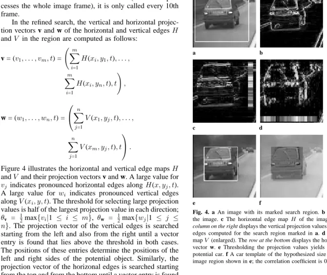
In the refined search, the vertical and horizontal projec-tion vectors v and w of the horizontal and vertical edgesH andV in the region are computed as follows:
v = (v1, . . . , vm, t) = m i=1 H(xi, y1, t), . . . , m i=1 H(xi, yn, t), t , w = (w1, . . . , wn, t) = n j=1 V(x1, yj, t), . . . , n j=1 V(xm, yj, t), t .
Figure 4 illustrates the horizontal and vertical edge mapsH andV and their projection vectors v and w. A large value for vj indicates pronounced horizontal edges along H(x, yj, t). A large value for wi indicates pronounced vertical edges alongV(xi, y, t). The threshold for selecting large projection values is half of the largest projection value in each direction; θv = 12max{vi|1 ≤ i ≤ m}, θw = 12max{wj|1 ≤ j ≤
n}. The projection vector of the vertical edges is searched starting from the left and also from the right until a vector entry is found that lies above the threshold in both cases. The positions of these entries determine the positions of the left and right sides of the potential object. Similarly, the projection vector of the horizonal edges is searched starting from the top and from the bottom until a vector entry is found that lies above the threshold in both cases. The positions of these entries determine the positions of the top and bottom sides of the potential object.
To verify that the potential object is a car, an objective function is evaluated as follows. First, the aspect ratio of the horizontal and vertical sides of the potential object is computed to check if it is close enough to 1 to imply that a car is detected. Then the car template is correlated with the potential object marked by the four corner points in the image. If the correlation yields a high value, the object is recognized as a car. The system outputs the fact that a car is detected, its location in the image, and its size.
4.3 Recognition by tracking
The previous sections described methods for recognizing cars from single images or image pairs. If an object can-not be recognized from one or two images immediately, our system evaluates several more consecutive image frames and employs its tracking capabilities to recognize vehicles.
The process coordinator creates a separate tracking pro-cess for each potential car (see Fig. 1). It uses the initial parameters for the position and size of the potential car that are determined by the car detector and ensures that no other
a b
c d
e f
Fig. 4. a An image with its marked search region. b The edge map of the image. c The horizontal edge mapH of the image (enlarged). The
column on the right displays the vertical projection values v of the horizontal
edges computed for the search region marked in a. d The vertical edge mapV (enlarged). The row at the bottom displays the horizontal projection vector w. e Thresholding the projection values yields the outline of the potential car. f A car template of the hypothesized size is overlaid on the image region shown in e; the correlation coefficient is 0.74
process is tracking the same image area. The tracker creates a “tracking window” that contains the potential car and is used to evaluate edge maps, features and templates in sub-sequent image frames. The position and size of the tracking window in subsequent frames is determined by a simple re-cursive filter: the tracking window in the current frame is the window that contains the potential car found in the previ-ous frame plus a boundary that surrounds the car. The size of this boundary is determined adaptively. The outline of the potential car within the current tracking window is com-puted by the refined feature search described in Sect. 4.2. As a next step, a template of a size that corresponds to the hy-pothesized size of the vehicle is created from a stored model image as described in Sect. 4.1. The template is correlated with the image region that is hypothesized to contain the ve-hicle (see Fig. 4f). If the normalized correlation of the image region and the template is high and typical vehicle motion and feature parameters are found, it is inferred that a vehicle is detected. Note that the normalized correlation coefficient is invariant to constant scale factors in brightness and can therefore adapt to the lighting conditions of a particular im-age frame. The model imim-ages shown in Sect. 4.1 are only used to create car templates on line as long as the tracked object is not yet recognized to be a vehicle; otherwise, the
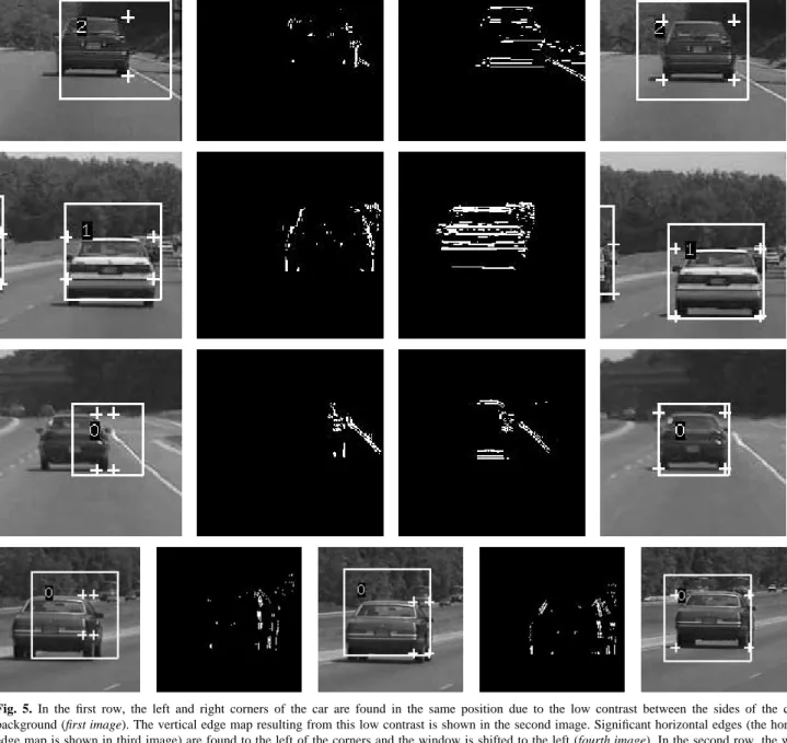
Fig. 5. In the first row, the left and right corners of the car are found in the same position due to the low contrast between the sides of the car and background (first image). The vertical edge map resulting from this low contrast is shown in the second image. Significant horizontal edges (the horizontal edge map is shown in third image) are found to the left of the corners and the window is shifted to the left (fourth image). In the second row, the window shift compensates for a 10-pixel downward motion of the camera due to uneven pavement. In the third row, the car passed underneath a bridge, and the tracking process is slowly “recovering.” The tracking window no longer contains the whole car, and its vertical edge map is therefore incomplete (second
image). However, significant horizontal edges (third image) are found to the left of the corners and the window is shifted to the left. In the last row, a
passing car is tracked incompletely. First its bottom corners are adjusted, then its left side
model is created on line by cropping the currently tracked vehicle.
4.3.1 Online model creation
The outline of the vehicle found defines the boundary of the image region that is cropped from the scene. This cropped region is then used as the model vehicle image, from which templates are created that are matched with subsequent im-ages. The templates created from such a model usually cor-relate extremely well (e.g., 90%), even if their sizes
substan-tially differ from the cropped model, and even after some image frames have passed since the model was created. As long as these templates yield high correlation coefficients, the vehicle is tracked correctly with high probability. As soon as a template yields a low correlation coefficient, it can be deduced automatically that the outline of the vehicle is not found correctly. Then the evaluation of subsequent frames either recovers the correct vehicle boundaries or ter-minates the tracking process.
4.3.2 Symmetry check
In addition to correlating the tracked image portion with a previously stored or cropped template, the system also checks for the portion’s left-right symmetry by correlating its left and right image halves. Highly symmetric image por-tions with typical vehicle features indicate that a vehicle is tracked correctly.
4.3.3 Objective function
In each frame, the objective function evaluates how likely it is that the object tracked is a car. It checks the “credit and penalty values” associated with each process. Credit and penalty values are assigned depending on the aspect ratio, size, and, if applicable, correlation for the tracking window of the process. For example, if the normalized correlation coefficient is larger than 0.6 for a car template of≥30×30 pixels, ten credits are added to the accumulated credit of the process, and the accumulated penalty of the process is set to zero. If the normalized correlation coefficient for a process is negative, the penalty associated with this process is in-creased by five units. Aspect ratios between 0.7 and 1.4 are considered to be potential aspect ratios of cars; one to three credits are added to the accumulated credit of the process (the number increases with the template size). If the accu-mulated credit is above a threshold (ten units) and exceeds the penalty, it is decided that the tracked object is a car. These values for the credit and penalty assignments seem somewhat ad hoc, but their selection was driven by careful experimental analysis. Examples of accumulated credits and penalties are given in the next section in Fig. 10.
A tracked car is no longer recognized if the penalty ex-ceeds the credit by a certain amount (three units). The track-ing process then terminates. A process also terminates if not enough significant edges are found within the tracking dow for several consecutive frames. This ensures that a win-dow that tracks a distant car does not “drift away” from the car and start tracking something else.
The process coordinator ensures that two tracking pro-cesses do not track objects that are too close to each other in the image. This may happen if a car passes another car and eventually occludes it. In this case, the process coordinator terminates one of these processes.
Processes that track unrecognized objects terminate them-selves if the objective function yields low values for several consecutive image frames. This ensures that oncoming traf-fic or objects that appear on the side of the road, such as traffic signs, are not falsely recognized and tracked as cars (see, for example, process 0 in frame 4 in Fig. 9).
4.3.4 Adaptive window adjustments
An adaptive window adjustment is necessary if – after a vehicle has been recognized and tracked for a while – its correct current outline is not found. This may happen, for example, if the rear window of the car is mistaken to be the whole rear of the car, because the car bottom is not contained in the current tracking window (the camera may have moved
up abruptly). Such a situation can be determined easily by searching along the extended left and right side of the car for significant vertical edges. In particular, the pixel values in the vertical edge map that lie between the left bottom corner of the car and the left bottom border of the window, and the right bottom corner of the car and the right bottom border of the window, are summed and compared with the corresponding sum on the top. If the sum on the bottom is significantly larger than the sum on the top, the window is shifted towards the bottom (it still includes the top side of the car). Similarly, if the aspect ratio is too small, the correct positions of the car sides are found by searching along the extended top and bottom of the car for significant horizontal edges, as illustrated in Fig. 5.
The window adjustments are useful for capturing the outline of a vehicle, even if the feature search encounters thresholding problems due to low contrast between the ve-hicle and its environment. The method supports recognition of passing cars that are not fully contained within the track-ing window, and it compensates for the up and down motion of the camera due to uneven pavement. Finally, it ensures that the tracker does not lose a car even if the road curves.
Detecting the rear lights of a tracked object, as described in the following paragraph, provides additional information that the system uses to identify the object as a vehicle. This is benefical in particular for reduced visibility driving, e.g. in a tunnel, at night, or in snowy conditions.
4.4 Rear-light detection
The rear-light detection algorithm searches for bright spots in image regions that are most likely to contain rear lights, in particular, the middle 3/5 and near the sides of the tracking windows. To reduce the search time, only the red component of each image frame is analyzed, which is sufficient for rear-light detection.
The algorithm detects the rear lights by looking for a pair of bright pixel regions in the tracking window that exceeds a certain threshold. To find this pair of lights and the centroid of each light, the algorithm exploits the symmetry of the rear lights with respect to the vertical axis of the tracking window. It can therefore eliminate false rear-light candidates that are due to other effects, such as specular reflections or lights in the background.
For windows that track cars at less than 10 m distance, a threshold that is very close to the brightest possible value 255, e.g. 250, is used, because at such small distances bright rear lights cause “blooming effects” in CCD cameras, espe-cially in poorly lit highway scenes, at night or in tunnels. For smaller tracking windows that contain cars at more than 10 m distance, a lower threshold of 200 was chosen experi-mentally.
Note that we cannot distinguish rear-light and rear-break-light detection, because the position of the rear rear-break-lights and the rear break lights on a car need not be separated in the US. This means that our algorithm finds either rear lights (if turned on) or rear break lights (when used). Fig-ures 11 and 12 illustrate rear-light detection results for typ-ical scenes.
model are used to obtain distance estimates. The coordinate origin of the 3D world coordinate system is placed at the pin-hole, theX- andY-coordinate axes are parallel to the image coordinate axes xandy, and theZ-axis is placed along the optical axis. Highway lanes usually have negligible slopes along the width of each lane, so we can assume that the camera’s pitch angle is zero if the camera is mounted hori-zontally level inside the car. If it is also placed at zero roll and yaw angles, the actual roll angle depends on the slope along the length of the lane, i.e., the highway inclination, and the actual yaw angle depends on the highway’s curva-ture. Given conversion factorschoriz andcvert from pixels to millimeters for our camera and estimates of the widthW and heightH of a typical car, we use the perspective equa-tions Z = chorizf W/w and Z = cvert f H/h, where Z is the distance between the camera-assisted car and the car that is being tracked in meters,wis the estimated car width andhthe estimated car height in pixels, andf is the focal length in millimeters. Given our assumptions, the distance estimates are most reliable for typically sized cars that are tracked immediately in front of the camera-assisted car.
5 Road color analysis
The previous sections discussed techniques for detecting and tracking vehicles based on the image brightness, i.e., gray-scale values and their edges. Edge maps carry information about road boundaries and obstacles on the road, but also about illumination changes on the roads, puddles, oil stains, tire skid marks, etc. Since it is very difficult to find good threshold values to eliminate unnecessary edge information, additional information provided by the color components of the input images is used to define these threshold values dy-namically. In particular, a statistical model for “road color” was developed, which is used to classify the pixels that im-age the road and discriminate them from pixels that imim-age obstacles such as other vehicles.
To obtain a reliable statistical model of road color, im-age regions are analyzed that consist entirely of road pix-els, for example, the black-bordered road region in the top image in Fig. 6, and regions that also contain cars, traffic signs, and road markings, e.g., the white-bordered region in the same image. Comparing the estimates for the mean and variance of red, green, and blue road pixels to respective es-timates for nonroad pixels does not yield a sufficient classi-fication criterion. However, an HSV = (hue, saturation, gray
value) representation [24] of the color input image proves
more effective for classification. Figure 6 illustrates such an HSV representation. In our data, the hue and saturation components give uniform representations of regions such as pavement, trees and sky, and eliminate the effects of un-even road conditions, but highlight car features, such as rear lights, traffic signs, lane markings, and road boundaries as can be seen, for example, in Fig. 6. Combining the hue and saturation information therefore yields an image representa-tion that enhances useful features and suppresses undesired ones. In addition, combining hue and saturation information
Fig. 6. The black-bordered road region in the top image is used to estimate the sample mean and variance of road color in the four images below. The
middle left image illustrates the hue component of the color image above,
the middle right illustrates the saturation component. The images at the
bottom are the gray-scale component and the composite image, which is
comprised of the sum of the horizontal and vertical brightness edge maps, hue and saturation images
with horizontal and vertical edge maps into a “composite
image,” provides the system with a data representation that
is extremely useful for highway scene analysis. Figure 6 shows a composite image in the bottom right. Figure 7 il-lustrates that thresholding pixels in the composite image by the mean (mean±3∗standard deviation) yields 96% correct
classification.
In addition, a statistical model for “daytime sky color” is computed off line and then used on line to distinguish daytime scenes from tunnel and night scenes.
6 Boundary and lane detection
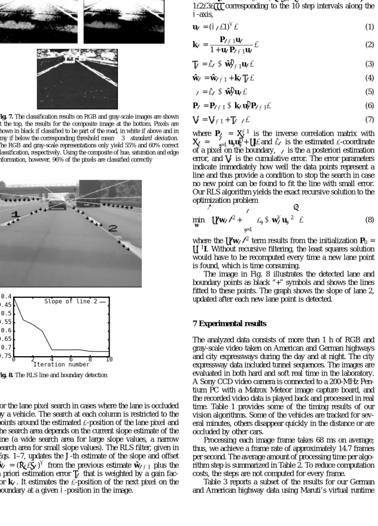
Road boundaries and lane markings are detected by a spatial recursive least squares filter (RLS) [33] with the main goal of guiding the search for vehicles. A linear model (y=ax+b) is used to estimate the slope a and offset b of lanes and road boundaries. This first-order model proved sufficient in guiding the vehicle search.
For the filter initialization, the left and right image boundaries are searched for a collection of pixels that do not fit the statistical model of road color and are there-fore classified to be potential initial points for lane and road boundaries. After obtaining initial estimates foraandb, the boundary detection algorithm continues to search for pix-els that do not satisfy the road color model at every 10th image column. In addition, each such pixel must be accom-panied to the below by a few pixels that satisfy the road color model. This restriction provides a stopping condition
Fig. 7. The classification results on RGB and gray-scale images are shown at the top, the results for the composite image at the bottom. Pixels are shown in black if classified to be part of the road, in white if above and in gray if below the corresponding threshold mean±3∗standard deviation.
The RGB and gray-scale representations only yield 55% and 60% correct classification, respectively. Using the composite of hue, saturation and edge information, however, 96% of the pixels are classified correctly
-0.75 -0.7 -0.65 -0.6 -0.55 -0.5 -0.45 -0.4 0 2 4 6 8 10 Iteration number Slope of line 2
Fig. 8. The RLS line and boundary detection
for the lane pixel search in cases where the lane is occluded by a vehicle. The search at each column is restricted to the points around the estimatedy-position of the lane pixel and the search area depends on the current slope estimate of the line (a wide search area for large slope values, a narrow search area for small slope values). The RLS filter, given in Eqs. 1–7, updates the n-th estimate of the slope and offset
ˆ
wn = ( ˆan,ˆbn)T from the previous estimate ˆwn−1 plus the
a priori estimation error ξn that is weighted by a gain fac-tor kn. It estimates the y-position of the next pixel on the boundary at a givenx-position in the image.
The algorithm is initialized by setting P0 = δ−1I, δ =
10−3, ε
0 = 0, wˆ0 = ( ˆa0,bˆ0)T. For each iteration n =
1,2,3, . . . corresponding to the 10 step intervals along the x-axis, un= (xn,1)T, (1) kn= Pn−1un 1 + unPn−1un, (2) ξn = ˆyn−wˆtn−1un, (3) ˆ wn= ˆwn−1+ knξn, (4) en= ˆyn−wˆtnun, (5) Pn= Pn−1−knutnPn−1, (6) εn=εn−1+ξnen, (7) where Pn = Φ−1
n is the inverse correlation matrix with Φn = ni=1uiuit+δI, and ˆyn is the estimatedy-coordinate
of a pixel on the boundary,en is the a posteriori estimation error, andεn is the cumulative error. The error parameters indicate immediately how well the data points represent a line and thus provide a condition to stop the search in case no new point can be found to fit the line with small error. Our RLS algorithm yields the exact recursive solution to the optimization problem min wn δwn2+ n i=1 |yi−wTnui|2 , (8)
where the δwn2 term results from the initialization P0 =
δ−1I. Without recursive filtering, the least squares solution
would have to be recomputed every time a new lane point is found, which is time consuming.
The image in Fig. 8 illustrates the detected lane and boundary points as black “+” symbols and shows the lines fitted to these points. The graph shows the slope of lane 2, updated after each new lane point is detected.
7 Experimental results
The analyzed data consists of more than 1 h of RGB and gray-scale video taken on American and German highways and city expressways during the day and at night. The city expressway data included tunnel sequences. The images are evaluated in both hard and soft real time in the laboratory. A Sony CCD video camera is connected to a 200-MHz Pen-tium PC with a Matrox Meteor image capture board, and the recorded video data is played back and processed in real time. Table 1 provides some of the timing results of our vision algorithms. Some of the vehicles are tracked for sev-eral minutes, others disappear quickly in the distance or are occluded by other cars.
Processing each image frame takes 68 ms on average; thus, we achieve a frame rate of approximately 14.7 frames per second. The average amount of processing time per algo-rithm step is summarized in Table 2. To reduce computation costs, the steps are not computed for every frame.
Table 3 reports a subset of the results for our German and American highway data using Maruti’s virtual runtime
0 20 40 60 80 100 120 140 160 180 200 20 40 60 80 100 120 140 160 180 200
x-coordinates of three detected cars
frame number
Fig. 9. Example of an image sequence in which cars are recognized and tracked. At the top, images are shown with their frame numbers in their lower right corners. The black rectangles show regions within which moving objects are detected. The corners of these objects are shown as crosses. The rectangles and crosses turn white when the system recognizes these objects to be cars. The graph at the bottom shows thex-coordinates of the positions of the three recognized cars
Table 1. Duration of vehicle tracking Tracking time No. of Average
vehicles time
<1 min 41 20 s
1–2 min 5 90 s
2–3 min 6 143 s
3–7 min 5 279 s
environment. During this test, a total of 48 out of 56 cars are detected and tracked successfully. Since the driving speed on American highways is much slower than on German
high-Table 2. Average processing time
Step Time Average time
Searching for potential cars 1–32 ms 14 ms Feature search in window 2–22 ms 13 ms Obtaining template 1–4 ms 2 ms Template match 2–34 ms 7 ms Lane detection 15–23 ms 18 ms
ways, less motion is detectable from one image frame to the next and not as many frames need to be processed.
0 50 100 150 200 250 300 0 20 40 60 80 100 120 140 160 180 200
Corner positions of process 0
frame number Sequence 1: Process 0 "top" "bottom" "right" "left" 0 20 40 60 80 100 120 0 20 40 60 80 100 120 140 160 180 200 Situation assessment frame number Sequence 1: Process 0 "detected" "credits" "penalties" 0 50 100 150 200 250 300 0 20 40 60 80 100 120 140 160 180 200
Corner positions of process 1
frame number Sequence 1: Process 1 "top" "bottom" "right" "left" 0 10 20 30 40 50 60 0 20 40 60 80 100 120 140 160 180 200 Situation assessment frame number Sequence 1: Process 1 "detected" "credits" "penalties" 0 50 100 150 200 250 0 20 40 60 80 100 120 140 160 180 200
Corner positions of process 2
frame number Sequence 1: Process 2 "top" "bottom" "right" "left" 0 20 40 60 80 100 120 140 0 20 40 60 80 100 120 140 160 180 200 Situation assessment frame number Sequence 1: Process 2 "detected" "credits" "penalties"
Fig. 10. Analysis of the sequence in Fig. 9: The graphs at the left illustrate they-coordinates of the top and bottom and thex-coordinates of the left and right corners of the tracking windows of processes 0, 1, and 2, respectively. In the beginning, the processes are created several times to track potential cars, but are quickly terminated, because the tracked objects are recognized not to be cars. The graphs at the right show the credit and penalty values associated with each process and whether the process has detected a car. A tracking process terminates after its accumulated penalty values exceed its accumulated credit values. As seen in the top graphs and in Fig. 9, process 0 starts tracking the first car in frame 35 and does not recognize the right and left car sides properly in frames 54 and 79. Because the car sides are found to be too close to each other, penalties are assessed in frames 54 and 79
Table 3. Detection and tracking results on gray-scale video
Data origin German American
Total number of frames ca. 5572 9670
No. of frames processed (in parentheses: every 2nd every 6th every 10th results normalized for every frame)
Detected and tracked cars 23 20 25
Cars not tracked 5 8 3
Size of detected cars (in pixels) 10×10–80×80 10×10–80×80 20×20–100×80 Avg. No. of frames during tracking 105.6 (211.2) 30.6 (183.6) 30.1 (301) Avg. No. of frames until car tracked 14.4 (28.8) 4.6 (27.6) 4.5 (45) Avg. No. of frames until stable detection 7.3 (14.6) 3.7 (22.2) 2.1 (21)
0 50 100 150 200 0 50 100 150 200 250 300 350 x coordinates, process 0 frame number "l" "r" "ll" "rl" 0 20 40 60 80 100 120 140 160 180 0 50 100 150 200 250 300 350 y coordinates, process 0 frame number "car bottom" "rear lights" 0 5 10 15 20 25 30 35 40 45 50 0 50 100 150 200 250 300 350 car distances frame number "process 0" "process 1"
Fig. 11. Detecting and tracking two cars on a snowy highway. In frame 3, the system determines that the data is taken at daytime. The black rectangles show regions within which moving objects are detected. Gray crosses indicate the top of the cars and white crosses indicate the bottom left and right car corners and rear light positions. The rectangles and crosses turn white when the system recognizes these objects to be cars. Underneath the middle image row, one of the tracking processes is illustrated in three ways: on the left, the vertical edge map of the tracked window is shown, in the middle, pixels identified not to belong to the road, but instead to an obstacle, are shown in white, and on the right, the most recent template used to compute the normalized correlation is shown. The text underneath shows the most recent correlation coefficient and distance estimate. The three graphs underneath the image sequence show position estimates. The left graph shows thex-coordinates of the left and right side of the left tracked car (“l” and “r”) and thex-coordinates of its left and right rear lights (“ll” and “rl”). The middle graph shows they-coordinates of the bottom side of the left tracked car (“car bottom”) and they-coordinates of its left and right rear lights (“rear lights”). The right graph shows the distance estimates for both cars
Figure 9 shows how three cars are recognized and tracked in an image sequence taken on a German highway. The graphs in Fig. 10 illustrate how the tracking processes are analyzed. Figures 11 and 12 show results for sequences in reduced visibility due to snow, night driving, and a tun-nel. These sequences were taken on an American highway and city expressway.
The lane and road boundary detection algorithm was tested by visual inspection on 14 min. of data taken on a two-lane highway under light-traffic conditions at daytime. During about 75% of the time, all the road lanes or
bound-aries are detected and tracked (three lines); during the re-maining time, usually only one or two lines are detected.
8 Discussion and conclusions
We have developed and implemented a hard real-time vision system that recognizes and tracks lanes, road boundaries, and multiple vehicles in videos taken from a car driving on German and American highways. Our system is able to run in real time with simple, low-cost hardware. All we rely on
Fig. 12. Detecting and tracking cars at night and in a tunnel (see caption of previous figure for color code). The cars in front of the camera-assisted car are detected and tracked reliably. The front car is detected and identified as a car at frame 24 and tracked until frame 260 in the night sequence, and identified at frame 14 and tracked until frame 258 in the tunnel sequence. The size of the cars in the other lanes are not detected correctly (frame 217 in night sequence and frame 194 in tunnel sequence)
is an ordinary video camera and a PC with an image capture board.
The vision algorithms employ a combination of bright-ness, hue and saturation information to analyze the high-way scene. Highhigh-way lanes and boundaries are detected and tracked using a recursive least squares filter. The highway scene is segmented into regions of interest, the “tracking windows,” from which vehicle templates are created on line and evaluated for symmetry in real time. From the track-ing and motion history of these windows, the detected fea-tures and the correlation and symmetry results, the system infers whether a vehicle is detected and tracked.
Experimen-tal results demonstrate robust, real-time car recognition and tracking over thousands of image frames, unless the system encounters uncooperative conditions, e.g., too little bright-ness contrast between the cars and the background, which sometime occurs at daytime, but often at night, and in very congested traffic. Under reduced visibility conditions, the system works well on snowy highways, at night when the background is uniformly dark, and in certain tunnels. How-ever, at night on city expressways, when there are many city lights in the background, the system has problems finding vehicle outlines and distinguishing vehicles on the road from obstacles in the background. Traffic congestion worsens the
the cars or misidentifies the sizes of the cars in adjacent lanes. If a precise 3D site model of the adjacent lanes and the highway background could be obtained and incorporated into the system, more reliable results in these difficult con-ditions could be expected.
Acknowledgements. The authors thank Prof. Ashok Agrawala and his group
for support with the Maruti operating system and the German Department of Transportation for providing the European data. The first author thanks her Boston College students Huan Nguyen for implementing the break-light detection algorithm, and Dewin Chandra and Robert Hatcher for helping to collect and digitize some of the data.
References
1. Aste M, Rossi M, Cattoni R, Caprile B (1998) Visual routines for real-time monitoring of vehicle behavior. Mach Vision Appl, 11:16–23 2. Batavia P, Pomerleau D, Thorpe C (1997) Overtaking vehicle detection
using implicit optical flow. In: Proceedings of the IEEE Conference on Intelligent Transportation Systems, Boston, Mass., November 1997, p 329
3. Behringer R, H¨otzel S (1994) Simultaneous estimation of pitch angle and lane width from the video image of a marked road. In: Proceedings of IEEE/RSJ/GI International Conference on Intelligent Robots and Systems, Munich, Germany, September 1994, pp 966–973
4. Bertozzi M, Broggi A (1997) Vision-based vehicle guidance. IEEE Comput 30(7), pp 49–55
5. Bertozzi M, Broggi A (1998) GOLD: A parallel real-time stereo vision system for generic obstacle and lane detection. IEEE Trans Image Process, 7(1):62–81
6. Betke M, Haritaoglu E, Davis L (1996) Multiple vehicle detection and tracking in hard real time. In Proceedings of the Intelligent Vehicles Symposium, Tokyo, Japan, September 1996. IEEE Industrial Electron-ics Society, Piscataway, N.J., pp 351–356
7. Betke M, Haritaoglu E, Davis LS (1997) Highway scene analysis in hard real time. In: Proceedings of the IEEE Conference on Intelligent Transportation Systems, Boston, Mass., November 1997, p 367 8. Betke M, Makris NC (1995) Fast object recognition in noisy images
using simulated annealing. In: Proceedings of the Fifth International Conference on Computer Vision, Cambridge, Mass., June 1995. IEEE Computer Society, Piscataway, N.J., pp 523–530
9. Betke M, Makris NC (1998) Information-conserving object recogni-tion. In: Proceedings of the Sixth International Conference on Com-puter Vision, Mumbai, India, January 1998. IEEE ComCom-puter Society, Piscataway, N.J., pp 145–152
10. Betke M, Nguyen H (1998) Highway scene analysis from a moving vehicle under reduced visibility conditions. In: Proceedings of the International Conference on Intelligent Vehicles, Stuttgart, Germany, October 1998. IEEE Industrial Electronics Society, Piscataway, N.J., pp 131–136
11. Beymer D, Malik J (1996) Tracking vehicles in congested traffic. In: Proceedings of the Intelligent Vehicles Symposium, Tokyo, Japan, 1996. IEEE Industrial Electronics Society, Piscataway, N.J., pp 130– 135
12. Beymer D, McLauchlan P, Coifman B, Malik J (1997) A real-time computer vision system for measuring traffic parameters. In: Proceed-ings of the IEEE Computer Vision and Pattern Recognition Confer-ence, Puerto Rico, June 1997. IEEE Computer Society, Piscataway, N.J., pp 495–501
13. Bohrer S, Zielke T, Freiburg V (1995) An integrated obstacle detection framework for intelligent cruise control on motorways. In: Proceed-ings of the Intelligent Vehicles Symposium, Detroit, MI, 1995. IEEE Industrial Electronics Society, Piscataway, N.J., pp 276–281 14. Broggi A (1995) Parallel and local feature extraction: A real-time
approach to road boundary detection. IEEE Trans Image Process, 4(2):217–223
Guidance: The Experience of the ARGO Autonomous Vehicle. World Scientific, Singapore
17. Crisman JD, Thorpe CE (1993) SCARF: A color vision system that tracks roads and intersections. IEEE Trans Robotics Autom, 9:49–58 18. Dellaert F, Pomerleau D, Thorpe C (1998) Model-based car tracking
integrated with a road-follower. In: Proceedings of the International Conference on Robotics and Automation, May 1998, IEEE Press, Pis-cataway, N.J., pp 197–202
19. Dellaert F, Thorpe C (1997) Robust car tracking using Kalman filtering and Bayesian templates. In: Proceedings of the SPIE Conference on Intelligent Transportation Systems, Pittsburgh, Pa, volume 3207, SPIE, 1997, pp 72–83
20. Dickmanns ED, Graefe V (1988) Applications of dynamic monocular machine vision. Mach Vision Appl 1(4):241–261
21. Dickmanns ED, Graefe V (1988) Dynamic monocular machine vision. Mach Vision Appl 1(4):223–240
22. Dickmanns ED, Mysliwetz BD (1992) Recursive 3-D road and relative ego-state recognition. IEEE Trans Pattern Anal Mach Intell 14(2):199– 213
23. Fathy M, Siyal MY (1995) A window-based edge detection technique for measuring road traffic parameters in real-time. Real-Time Imaging 1(4):297–305
24. Foley JD, van Dam A, Feiner SK, Hughes JF (1996) Computer Graph-ics: Principles and Practice. Addison-Wesley, Reading, Mass. 25. Franke U, B¨ottinger F, Zomoter Z, Seeberger D (1995) Truck
pla-tooning in mixed traffic. In: Proceedings of the Intelligent Vehicles Symposium, Detroit, MI, September 1995. IEEE Industrial Electronics Society, Piscataway, N.J., pp 1–6
26. Gengenbach V, Nagel H-H, Heimes F, Struck G, Kollnig H (1995) Model-based recognition of intersection and lane structure. In: Proceed-ings of the Intelligent Vehicles Symposium, Detroit, MI, September 1995. IEEE Industrial Electronics Society, Piscataway, N.J., pp 512– 517
27. Giachetti A, Cappello M, Torre V (1995) Dynamic segmentation of traffic scenes. In: Proceedings of the Intelligent Vehicles Symposium, Detroit, MI, September 1995. IEEE Computer Society, Piscataway, N.J., pp 258–263
28. Gil S, Milanese R, Pun T (1996) Combining multiple motion esti-mates for vehicle tracking. In: Lecture Notes in Computer Science. Vol. 1065: Proceedings of the 4th European Conference on Computer Vision, volume II, Springer, Berlin Heidelberg New York, April 1996, pp 307–320
29. Gillner WJ (1995) Motion based vehicle detection on motorways. In: Proceedings of the Intelligent Vehicles Symposium, Detroit, MI, September 1995. IEEE Industrial Electronics Society, Piscataway, N.J., pp 483–487
30. Graefe V, Efenberger W (1996) A novel approach for the detection of vehicles on freeways by real-time vision. In: Proceedings of the Intelligent Vehicles Symposium, Tokyo, Japan, 1996. IEEE Industrial Electronics Society, Piscataway, N.J., pp 363–368
31. Haga T, Sasakawa K, Kuroda S (1995) The detection of line bound-ary markings using the modified spoke filter. In: Proceedings of the Intelligent Vehicles Symposium, Detroit, MI, September 1995. IEEE Industrial Electronics Society, Piscataway, N.J., pp 293–298 32. Hansson HA, Lawson HW, Str¨omberg M, Larsson S (1996)
BASE-MENT: A distributed real-time architecture for vehicle applications. Real-Time Systems 11:223–244
33. Haykin S (1991) Adaptive Filter Theory. Prentice Hall
34. Hsu J-C, Chen W-L, Lin R-H, Yeh EC (1997) Estimations of previewd road curvatures and vehicular motion by a vision-based data fusion scheme. Mach Vision Appl 9:179–192
35. Ikeda I, Ohnaka S, Mizoguchi M (1996) Traffic measurement with a roadside vision system – individual tracking of overlapped vehicles. In: Proceedings of the 13th International Conference on Pattern Recog-nition, volume 3, pp 859–864
36. Jochem T, Pomerleau D, Thorpe C (1995) Vision guided lane-transition. In: Proceedings of the Intelligent Vehicles Symposium,
Detroit, Mich., September 1995. IEEE Industrial Electronics Society, Piscataway, N.J., pp 30–35
37. Kalinke T, Tzomakas C, von Seelen W (1998) A texture-based object detection and an adaptive model-based classification. In: Proceedings of the International Conference on Intelligent Vehicles, Stuttgart, Ger-many, October 1998. IEEE Industrial Electronics Society, Piscataway, N.J., pp 143–148
38. Kaminski L, Allen J, Masaki I, Lemus G (1995) A sub-pixel stereo vision system for cost-effective intelligent vehicle applications. In: Proceedings of the Intelligent Vehicles Symposium, Detroit, Mich., September 1995. IEEE Industrial Electronics Society, Piscataway, N.J., pp 7–12
39. Kluge K, Johnson G (1995) Statistical characterization of the visual characteristics of painted lane markings. In: Proceedings of the In-telligent Vehicles Symposium, Detroit, Mich., September 1995. IEEE Industrial Electronics Society, Piscataway, N.J., pp 488–493 40. Kluge K, Lakshmanan S (1995) A deformable-template approach to
line detection. In: Proceedings of the Intelligent Vehicles Symposium, Detroit, Mich., September 1995. IEEE Industrial Electronics Society, Piscataway, N.J., pp 54–59
41. Koller D, Weber J, Malik J (1994) Robust multiple car tracking with occlusion reasoning. In: Lecture Notes in Computer Science. Vol. 800: Proceedings of the 3rd European Conference on Computer Vision, volume I, Springer, Berlin Heidelberg New York, May 1994, pp 189– 196
42. Kr¨uger W (1999) Robust real-time ground plane motion compensation from a moving vehicle. Machine Vision and Applications, 11(4):203– 212
43. Kr¨uger W, Enkelmann W, R¨ossle S (1995) Real-time estimation and tracking of optical flow vectors for obstacle detection. In: Proceedings of the Intelligent Vehicles Symposium, Detroit, Mich., September 1995. IEEE Industrial Electronics Society, Piscataway, N.J., pp 304–309 44. Luong Q, Weber J, Koller D, Malik J (1995) An integrated
stereo-based approach to automatic vehicle guidance. In: Proceedings of the International Conference on Computer Vision, Cambridge, Mass., 1995. IEEE Computer Society, Piscataway, N.J., pp 52–57
45. Marmoiton F, Collange F, Derutin J-P, Alizon J (1998) 3D localization of a car observed through a monocular video camera. In: Proceedings of the International Conference on Intelligent Vehicles, Stuttgart, Ger-many, October 1998. IEEE Industrial Electronics Society, Piscataway, N.J., pp 189–194
46. Masaki I (ed.) (1992) Vision-based Vehicle Guidance. Springer, Berlin Heidelberg New York
47. Maurer M, Behringer R, F¨urst S, Thomarek F, Dickmanns ED (1996) A compact vision system for road vehicle guidance. In: Proceedings of the 13th International Conference on Pattern Recognition, volume 3, pp 313–317
48. NavLab, Robotics Institute, Carnegie Mellon University. http://www.ri.cmu.edu/labs/lab 28.html.
49. Ninomiya Y, Matsuda S, Ohta M, Harata Y, Suzuki T (1995) A real-time vision for intelligent vehicles. In: Proceedings of the Intelligent Vehicles Symposium, Detroit, Mich., September 1995. IEEE Industrial Electronics Society, Piscataway, N.J., pp 101–106
50. Noll D, Werner M, von Seelen W (1995) Real-time vehicle tracking and classification. In: Proceedings of the Intelligent Vehicles Symposium, Detroit, Mich., September 1995. IEEE Industrial Electronics Society, Piscataway, N.J., pp 101–106
51. Pomerleau D (1995) RALPH: Rapidly adapting lateral position han-dler. In: Proceedings of the Intelligent Vehicles Symposium, Detroit, Mich., 1995. IEEE Industrial Electronics Society, Piscataway, N.J., pp 506–511
52. Pomerleau D (1997) Visibility estimation from a moving vehicle using the RALPH vision system. In: Proceedings of the IEEE Conference on Intelligent Transportation Systems, Boston, Mass., November 1997, p 403
53. Redmill KA (1997) A simple vision system for lane keeping. In: Proceedings of the IEEE Conference on Intelligent Transportation Sys-tems, Boston, Mass., November 1997, p 93
54. Regensburger U, Graefe V (1994) Visual recognition of obstacles on roads. In: IEEE/RSJ/GI International Conference on Intelligent Robots and Systems, Munich, Germany, September 1994, pp 982–987 55. Rojas JC, Crisman JD (1997) Vehicle detection in color images. In:
Proceedings of the IEEE Conference on Intelligent Transportation Sys-tems, Boston, Mass., November 1997, p 173
56. Saksena MC, da Silva J, Agrawala AK (1994) Design and implementa-tion of Maruti-II. In: Sang Son (ed.) Principles of Real-Time Systems. Prentice-Hall, Englewood Cliffs, N.J.
57. Schneiderman H, Nashman M, Wavering AJ, Lumia R (1995) Vision-based robotic convoy driving. Machine Vision and Applications 8(6):359–364
58. Smith SM (1995) ASSET-2: Real-time motion segmentation and shape tracking. In: Proceedings of the International Conference on Computer Vision, Cambridge, Mass., 1995. IEEE Computer Society, Piscataway, N.J., pp 237–244
59. Thomanek F, Dickmanns ED, Dickmanns D (1994) Multiple object recognition and scene interpretation for autonomous road vehicle guid-ance. In: Proceedings of the Intelligent Vehicles Symposium, Paris, France, 1994. IEEE Industrial Electronics Society, Piscataway, N.J., pp 231–236
60. Thorpe CE (ed.) (1990) Vision and Navigation. The Carnegie Mellon Navlab. Kluwer Academic Publishers, Boston, Mass.
61. Willersinn D, Enkelmann W (1997) Robust obstacle detection and tracking by motion analysis. In: Proceedings of the IEEE Conference on Intelligent Transportation Systems, Boston, Mass., November 1997, p 325
62. Williamson T, Thorpe C (1999) A trinocular stereo system for highway obstacle detection. In: Proceedings of the International Conference on Robotics and Automation. IEEE, Piscataway, N.J.
63. Zielke T, Brauckmann M, von Seelen W (1993) Intensity and edge-based symmetry detection with an application to car-following. CVGIP: Image Understanding 58:177–190
Margrit Betke’s research area is computer vision, in particular, object recognition, med-ical imaging, real-time systems, and machine learning. Prof. Betke received her Ph. D. and S. M. degrees in Computer Science and Elec-trical Engineering from the Massachusetts Institute of Technology in 1995 and 1992, re-spectively. After completing her Ph. D. the-sis on “Learning and Vision Algorithms for Robot Navigation,” at MIT, she spent 2 years as a Research Associate in the Institute for Advanced Computer Studies at the Univer-sity of Maryland. She was also affiliated with the Computer Vision Laboratory of the Cen-ter for Automation Research at UMD. She has been an Assistant Professor at Boston College for 3 years and is a Research Scientist at the Massachusetts General Hospital and Harvard Medical School. In July 2000, she will join the Computer Science Department at Boston University.
Larry S. Davis received his B. A. from Colgate University in 1970 and his M. S. and Ph. D. in Computer Science from the University of Maryland in 1974 and 1976, respectively. From 1977 to 1981 he was an Assistant Pro-fessor in the Department of Computer Science at the University of Texas, Austin. He returned to the University of Maryland as an Associate
Pro-of the IEEE in 1997. PrPro-ofessor Davis is known for his research in computer vision and high-performance computing. He has published over 75 papers in journals and has supervised over 12 Ph. D. students. He is an Associate Editor of the International Journal of Computer Vision and an area editor for Computer Models for Image Processor: Image Understanding. He has served as program or general chair for most of the field’s major conferences and workshops, including the 5th International Conference on Computer Vision, the field’s leading international conference.