The DaCapo Benchmarks: Java Benchmarking Development and Analysis (Extended Version)

The DaCapo Benchmarks: Java Benchmarking Development and

Analysis (Extended Version)

∗

Stephen M Blackburn

, Robin Garner

, Chris Hoffmann

, Asjad M Khan

, Kathryn S McKinley

,

Rotem Bentzur

, Amer Diwan

, Daniel Feinberg

, Daniel Frampton

, Samuel Z Guyer

, Martin Hirzel

,

Antony Hosking

, Maria Jump

, Han Lee

, J Eliot B Moss

, Aashish Phansalkar

, Darko Stefanovi´c

,

Thomas VanDrunen

, Daniel von Dincklage

, Ben Wiedermann

α_Intel,β_{Australian National University,} γ_{University of Massachusetts at Amherst,}δ_{University of Texas at Austin,} ε_{University of New Mexico,}ζ_{University of Colorado,}η_Tufts,θ_{IBM TJ Watson Research Center,} ι_{Purdue University,}

κ_{Wheaton College}

Abstract

Since benchmarks drive computer science research and industry product development, which ones we use and how we evaluate them are key questions for the community. Despite complex run-time tradeoffs due to dynamic compilation and garbage collection required for Java programs, many evaluations still use methodolo-gies developed for C, C++, and Fortran. SPEC, the dominant pur-veyor of benchmarks, compounded this problem by institutionaliz-ing these methodologies for their Java benchmark suite. This paper recommends benchmarking selection and evaluation methodolo-gies, and introduces the DaCapo benchmarks, a set of open source, client-side Java benchmarks. We demonstrate that the complex in-teractions of (1) architecture, (2) compiler, (3) virtual machine, (4) memory management, and (5) application require more extensive evaluation than C, C++, and Fortran which stress (4) much less, and do not require (3). We use and introduce new value, time-series, and statistical metrics for static and dynamic properties such as code complexity, code size, heap composition, and pointer muta-tions. No benchmark suite is definitive, but these metrics show that DaCapo improves over SPEC Java in a variety of ways, including more complex code, richer object behaviors, and more demanding memory system requirements. This paper takes a step towards im-proving methodologies for choosing and evaluating benchmarks to foster innovation in system design and implementation for Java and other managed languages.

Categories and Subject Descriptors C.4 [Measurement Techniques] General Terms Measurement, Performance

Keywords methodology, benchmark, DaCapo, Java, SPEC

1.

Introduction

When researchers explore new system features and optimizations, they typically evaluate them with benchmarks. If the idea does not improve a set of interesting benchmarks, researchers are unlikely to submit the idea for publication, or if they do, the community is unlikely to accept it. Thus, benchmarks set standards for innovation and can encourage or stifle it.

∗_{This technical report is an extended version of [6].}

This work is supported by NSF ITR CCR-0085792, NSF CCR-0311829, NSF CCF-CCR-0311829, NSF CISE infrastructure grant EIA-0303609, ARC DP0452011, DARPA F33615-03-C-4106, DARPA NBCH30390004, IBM, and Intel. Any opinions, findings and conclusions expressed herein are those of the authors and do not necessarily reflect those of the sponsors.

For Java, industry and academia typically use the SPEC Java benchmarks (the SPECjvm98 benchmarks and SPECjbb2000 [37, 38]). When SPEC introduced these benchmarks, their evaluation rules and the community’s evaluation metrics glossed over some of the key questions for Java benchmarking. For example, (1) SPEC reporting of the “best” execution time is taken from multiple it-erations of the benchmark within a single execution of the virtual machine, which will typically eliminate compile time. (2) In ad-dition to steady state application performance, a key question for Java virtual machines (JVMs) is the tradeoff between compile and application time, yet SPEC does not require this metric, and the community often does not report it. (3) SPEC does not require re-ports on multiple heap sizes and thus does not explore the space-time tradeoff automatic memory management (garbage collection) must make. SPEC specifies three possible heap sizes, all of which over-provision the heap. Some researchers and industry evaluations of course do vary and report these metrics, but many do not.

This paper introduces the DaCapo benchmarks, a set of gen-eral purpose, realistic, freely available Java applications. This pa-per also recommends a number of methodologies for choosing and evaluating Java benchmarks, virtual machines, and their memory management systems. Some of these methodologies are already in use. For example, Eeckhout et al. recommend that hardware ven-dors use multiple JVMs for benchmarking because applications vary significantly based on JVM [19]. We recommend and use this methodology on three commercial JVMs, confirming none is a con-sistent winner and benchmark variation is large. We recommend here a deterministic methodology for evaluating compiler optimiza-tions that holds the compiler workload constant, as well as the stan-dard steady-state stable performance methodology. For evaluating garbage collectors, we recommend multiple heap sizes and deter-ministic compiler configurations. We also suggest new and previ-ous methodologies for selecting benchmarks and comparing them. For example, we recommend time-series data versus single values, including heap composition and pointer distances for live objects as well as allocated objects. We also recommend principal component analysis [13, 18, 19] to assess differences between benchmarks.

We use these methodologies to evaluate and compare DaCapo and SPEC, finding that DaCapo is more complex in terms of static and dynamic metrics. For example, DaCapo benchmarks have much richer code complexity, class structures, and class hierarchies than SPEC according to the Chidamber and Kemerer metrics [12]. Furthermore, this static complexity produces a wider variety and more complex object behavior at runtime, as measured by data structure complexity, pointer source/target heap distances, live and allocated object characteristics, and heap composition. Principal component analysis using code, object, and architecture behavior metrics differentiates all the benchmarks from each other.

The main contributions of this paper are new, more realistic Java benchmarks, an evaluation methodology for developing benchmark suites, and performance evaluation methodologies. Needless to say,

the DaCapo benchmarks are not definitive, and they may or may not be representative of workloads that vendors and clients care about most. Regardless, we believe this paper is a step towards a wider community discussion and eventual consensus on how to select, measure, and evaluate benchmarks, VMs, compilers, runtimes, and hardware for Java and other managed languages.

2.

Related Work

We build on prior methodologies and metrics, and go further to recommend how to use them to select benchmarks and for best practices in performance evaluation.

2.1 Java Benchmark Suites

In addition to SPEC (discussed in Section 3), prior Java bench-marks suites include Java Grande [26], Jolden [11, 34], and Ashes [17]. The Java Grande Benchmarks include programs with large demands for memory, bandwidth, or processing power [26]. They focus on array intensive programs that solve scientific com-puting problems. The programs are sequential, parallel, and dis-tributed. They also include microbenchmark tests for language and communication features, and some cross-language tests for com-paring C and Java. DaCapo also focuses on large, realistic pro-grams, but not on parallel or distributed programs. The DaCapo benchmarks are more general purpose, and include both client and server side applications.

The Jolden benchmarks are single-threaded Java programs rewritten from parallel C programs that use dynamic pointer data structures [11, 34]. These programs are small kernels (less than 600 lines of code) intended to explore pointer analysis and paralleliza-tion, not complete systems. The Soot project distributes the Ashes benchmarks with their Java compiler infrastructure, and include the Jolden benchmarks, a few more realistic benchmarks such as their compiler, and some interactive benchmarks [17]. The DaCapo benchmarks contain many more realistic programs, and are more ambitious in scope.

2.2 Benchmark Metrics and Characterization

Dufour et al. recommend characterizing benchmarks with architec-ture independent value metrics that summarize: (1) size and struc-ture of program, (2) data strucstruc-tures, (3) polymorphism, (4) memory, and (5) concurrency into a single number [17]. We do not consider concurrency metrics to limit the scope of our efforts. We use met-rics from the first four categories and add metmet-rics, such as filter-ing for just the live objects, that better expose application behavior. Our focus is on continuous metrics, such as pointer distributions and heap composition graphs, rather than single values. Dufour et al. show how to use these metrics to drive compiler optimization explorations, whereas we show how to use these metrics to develop methodologies for performance and benchmark evaluation.

Prior work studied some of the object properties we present here [4, 15, 21, 39], but not for the purposes of driving benchmark selection and evaluation methodologies. For example, Dieckmann and H¨olzle [15] measure object allocation properties, and we add to their analysis live object properties and pointer demographics. Stefanovi´c pioneered the use of heap composition graphs which we use here to show inherent object lifetime behaviors [39].

2.3 Performance Evaluation Methodologies

Eeckhout et al. study SPECjvm98 and other Java benchmarks using a number of virtual machines on one architecture, AMD’s K7 [19]. Their cluster analysis shows that methodologies for designing new hardware should include multiple virtual machines and benchmarks because each widely exercises different hardware aspects. One limitation of their work is that they use a fixed heap size, which as we show masks the interaction of the memory manager’s space-time tradeoff in addition to its influence on mutator locality. We

add to Eeckhout et al.’s good practices in methodology that the hardware designers should include multiple heap sizes and memory management strategies. We confirm Eeckhout et al.’s finding. We present results for three commercial JVMs on one architecture that show a wide range of performance sensitivities. No one JVM is best across the suite with respect to compilation time and code quality, and there is a lot a variation. These results indicate there is plenty of room for improving current commercial JVMs.

Many recent studies examine and characterize the behavior of Java programs in simulation or on hardware [19, 21, 23, 28, 29, 30, 31, 32, 33]. This work focuses on workload characterization, application behavior on hardware, and key differences with C pro-grams. For example, Hauswirth et al. mine application behavior to understand performance [21]. The bulk of our evaluation fo-cuses on benchmark properties that are independent of any particu-lar hardware or virtual machine implementation, whereas this prior work concentrates on how applications behave on certain hardware with one or more virtual machines. We extend these results to sug-gest that these characteristics can be used to separate and evaluate the benchmarks in addition to the software and hardware running them. Much of this Java performance analysis work either disables garbage collection [15, 35], which introduces unnecessary mem-ory fragmentation, or holds the heap size and/or garbage collector constant [19, 28], which may hide locality effects.

A number of researchers examine garbage collection and its in-fluence on application performance [3, 4, 20, 22, 28, 40]. For ex-ample, Kim and Hsu use multiple heap sizes and simulate different memory hierarchies with a whole heap mark-sweep algorithm, as-sisted by occasional compaction [28]. Kim and Hsu, and Rajan et al. [33] note that a mark-sweep collector has a higher miss rate than the application itself because the collector touches reachable data that may not be in the program’s current working set. Blackburn et al. use the methodology we recommend here for studying the influence of copying, mark-sweep, and reference counting collec-tors, and their generational variants on three architectures [4]. They show a contiguously allocating generational copying collector de-livers better mutator cache performance and total performance than a whole-heap mark-sweep collector with a free-list. A few studies explore heap size effects on performance [9, 10, 28], and as we show here, garbage collectors are very sensitive to heap size, and in particular to tight heaps. Diwan et al. [16, 41], Hicks et al. [22], and others [7, 8, 24] measure detailed, specific mechanism costs and architecture influences [16], but do not consider a variety of collection algorithms. Our work reflects these results and method-ologies, but makes additional recommendations.

3.

Benchmark and Methodology Introduction

This section describes SPEC Java and SPEC execution rules, how we collected DaCapo benchmarks, and our execution harness.

3.1 SPEC Java Benchmarks.

We compare the DaCapo suite to SPECjvm98 [37] and a modified version of SPECjbb2000 [38], and call them the SPEC Java bench-marks, or SPEC for short. We exclude SPECjAppServer because it requires multiple pieces of hardware and software to execute. The original SPECjbb2000 is a server-side Java application and reports its score as work done over a fixed time rather than elapsed time for a fixed work load. Although throughput (measuring work done over a fixed time) is one important criteria for understanding applica-tions such as transaction processing systems, most applicaapplica-tions are not throughput oriented. Superficially, the difference between fix-ing the time and workload is minor, however a variable workload is methodologically problematic. First, throughput workloads force a repetitive loop into the benchmark, which influences JIT optimiza-tion strategies and opportunities for parallelism, but is not represen-tative of the wide range of non-repetitive workloads. Furthermore,

variable workloads make performance hard to analyze and reason about. For example, the level and number of classes optimized and re-optimized at higher levels and the number of garbage collec-tions vary with the workload, leading to complex cascading effects on overall performance. We therefore modify SPECjbb2000, creat-ing pseudojbb, which executes a fixed workload (by default, 70,000 transactions execute against a single warehouse).

SPEC benchmarking rules discourage special casing the vir-tual machine, compiler, and/or architecture for a specific SPEC Java benchmark. They specify the largest input size (100), se-quencing through the benchmarks, no harness caching, and no pre-compilation of classes. The SPECjvm98 harness runs all the bench-marks multiple times, and intersperses untimed and timed execu-tions. Benchmarkers may run all the programs as many times as they like, and then report the best and worst results using the same virtual machine and compiler configurations. SPEC indicates that reporting should specify the memory sizes: 48MB, 48–256MB, and greater than 256MB, but does not require reporting all three. All these sizes over provision the heap. Excluding the virtual machine, SPEC programs allocate up to 271MB, and have at most 8MB live in the heap at any time, except for pseudojbb with 21MB live (see Section 7). Since 2000, none of the vendors has published results for the smaller heaps.

The SPEC committee is currently working on collecting a new set of Java benchmarks. The SPEC committee consists of industrial representatives and a few academics. One of their main criteria is representativeness, which industry is much better to judge than academia. When SPEC releases new benchmark sets, they include a performance comparison point. They do not include or describe any measured metrics on which they based their selection. This paper suggests methodologies for both selecting and evaluating Java Benchmarks, which are not being used or recommended in current industrial standards, SPEC or otherwise.

3.2 DaCapo Benchmarks

We began the DaCapo benchmarking effort in mid 2003 as the re-sult of an NSF review panel in which the panel and the DaCapo research group agreed that the existing Java benchmarks were lim-iting our progress. What followed was a two-pronged effort to iden-tify suitable benchmarks, and develop a suite of analyses to char-acterize candidate benchmarks and evaluate them for inclusion. We began with the following criteria.

1. Diverse real applications. We want applications that are widely used to provide a compelling focus for the community’s innova-tion and optimizainnova-tions, as compared to synthetic benchmarks. 2. Ease of use. We want the applications to be relatively easy to

use and measure.

We implemented these criteria as follows.

1. We chose only open source benchmarks and libraries.

2. We chose diverse programs to maximize coverage of application domains and application behaviors.

3. We focused on client-side benchmarks that are easy to measure in a completely standard way, with minimal dependences out-side the scope of the host JVM.

4. We excluded GUI applications since they are difficult to bench-mark systematically. In the case of eclipse, we exercise a non-GUI subset.

5. We provide a range of inputs. With the default input sizes, the programs are timely enough that it takes hours or days to execute thousands of invocations of the suite, rather than weeks. With the exception of eclipse, which runs for around a minute, each benchmark executes for between 5 and 20 seconds on contemporary hardware and JVMs.

We considered other potential criteria, such as long running, GUI, and client-server applications. We settled on the above character-istics because their focus is similar to the existing SPEC bench-marks, while addressing some of our key concerns. Around 20 stu-dents and faculty at six institutions then began an iterative process of identifying, preparing, and experimenting with candidate bench-marks. Realizing the difficulty of identifying a good benchmark suite, we made the DaCapo benchmark project open and transpar-ent, inviting feedback from the community [14]. As part of this process, we have released three beta versions.

We identified a broad range of static and dynamic metrics, including some new ones, and developed a framework in Jikes RVM [1] for performing these detailed analyses. Sections 6, 7, and 8 describe these metrics. We systematically analyzed each can-didate to identify ones with non-trivial behavior and to maximize the suite’s coverage. We included most of the benchmarks we eval-uated, excluding only a few that were too trivial or whose license agreements were too restrictive, and one that extensively used ex-ceptions to avoid explicit control flow.

The Constituent Benchmarks We now briefly describe each benchmark in the final pre-release of the suite (beta-2006-08) that we use throughout the paper. More detailed descriptions appear in Figures 4 through 22. The source code and the benchmark harness are available on the DaCapo benchmark web site [14].

antlr A parser generator and translator generator.

bloat A bytecode-level optimization and analysis tool for Java. chart A graph plotting toolkit and pdf renderer.

eclipse An integrated development environment (IDE). fop An output-independent print formatter.

hsqldb An SQL relational database engine written in Java. jython A python interpreter written in Java.

luindex A text indexing tool. lusearch A text search tool.

pmd A source code analyzer for Java.

xalan An XSLT processor for transforming XML documents.

The benchmark suite is packaged as a single jar file containing a harness (licensed under the Apache Public License [2]), all the benchmarks, the libraries they require, three input sizes, and input data (e.g., luindex, lusearch and xalan all use the works of Shake-speare). We experimented with different inputs and picked repre-sentative ones.

The Benchmark Harness We provide a harness to invoke the benchmarks and perform a validity check that insures each bench-mark ran to completion correctly. The validity check performs checksums onerrandoutstreams during benchmark execution and on any generated files after benchmark execution. The harness passes the benchmark if its checksums match pre-calculated values. The harness supports a range of options, including user-specified hooks to call at the start and end of the benchmark and/or after the benchmark warm-up period, running multiple benchmarks, and printing a brief summary of each benchmark and its origins. It also supports workload size (small, default, large), which iteration (first, second, or nth), or a performance-stable iteration for reporting ex-ecution time. To find a performance-stable iteration, the harness takes a window size w (number of executions) and a convergence target v, and runs the benchmark repeatedly until either the coef-ficient of variation,σ_µ, of the last w runs drops below v, or reports failure if the number of runs exceeds a maximum m (whereσis the standard deviation and µ is the arithmetic mean of the last w exe-cution times). Once performance stabilizes, the harness reports the execution time of the next iteration. The harness provides defaults for w and v, which the user may override.

1 1.2 1.4 1.6 1.8 2 2.2 2.4 1 2 3 4 5 6 10 20 30 40 50 60 70 80 90 Normalized Time

Heap size relative to minimum heap size Heap size (MB) PPC 1.6 SS PPC 1.6 MS P4 3.0 SS P4 3.0 MS AMD 2.2 SS AMD 2.2 MS PM 2.0 SS PM 2.0 MS (a) SPEC 1 1.2 1.4 1.6 1.8 2 2.2 2.4 1 2 3 4 5 6 50 100 150 200 Normalized Time

Heap size relative to minimum heap size Heap size (MB) PPC 1.6 SS PPC 1.6 MS P4 3.0 SS P4 3.0 MS AMD 2.2 SS AMD 2.2 MS PM 2.0 SS PM 2.0 MS (b) DaCapo

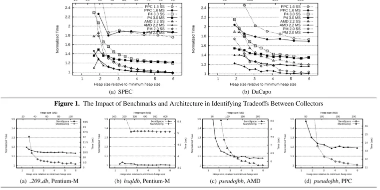
Figure 1. The Impact of Benchmarks and Architecture in Identifying Tradeoffs Between Collectors

1 1.1 1.2 1.3 1.4 1.5 1 2 3 4 5 6 9 9.5 10 10.5 11 11.5 12 12.5 13 13.5 20 40 60 80 100 Normalized Time Time (sec)

Heap size relative to minimum heap size Heap size (MB) SemiSpace MarkSweep (a) 209 db, Pentium-M 1 1.1 1.2 1.3 1.4 1.5 1 2 3 4 5 6 3.5 4 4.5 5 5.5 100 200 300 400 500 600 Normalized Time Time (sec)

Heap size relative to minimum heap size Heap size (MB) SemiSpace MarkSweep (b) hsqldb, Pentium-M 1 1.1 1.2 1.3 1.4 1.5 1 2 3 4 5 6 6 6.5 7 7.5 8 8.5 50 100 150 200 Normalized Time Time (sec)

Heap size relative to minimum heap size Heap size (MB) SemiSpace MarkSweep (c) pseudojbb, AMD 1 1.1 1.2 1.3 1.4 1.5 1 2 3 4 5 6 11 12 13 14 15 16 50 100 150 200 Normalized Time Time (sec)

Heap size relative to minimum heap size Heap size (MB)

SemiSpace MarkSweep

(d) pseudojbb, PPC

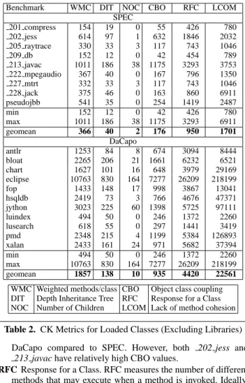
Figure 2. Gaming Your Results

4.

Virtual Machine Experimental Methodologies

We modified Jikes RVM [1] version 2.4.4+ to report static met-rics, dynamic metmet-rics, and performance results. We use this virtual machine because it is open source and performs well. Unless other-wise specified, we use a generational collector with a variable sized copying nursery and a mark-sweep older space because it is a high performance collector configuration [4], and consequently is popu-lar in commercial virtual machines. We call this collector GenMS. Our research group and others have used and recommended the fol-lowing methodologies to understand virtual machines, application behaviors, and their interactions.

Mix. The mix methodology measures an iteration of an

applica-tion which mixes JIT compilaapplica-tion and recompilaapplica-tion work with application time. This measurement shows the tradeoff of total time with compilation and application execution time. SPEC’s “worst” number may often, but is not guaranteed to, correspond to this measurement.

Stable. To measure stable application performance, researchers

typically report a steady-state run in which there is no JIT com-pilation and only the application and memory management sys-tem are executing. This measurement corresponds to the SPEC “best” performance number. It measures final code quality, but does not guarantee the compiler behaved deterministically.

Deterministic Stable & Mix. This methodology eliminates

sam-pling and recompilation as a source of non-determinism. It modifies the JIT compiler to perform replay compilation which applies a fixed compilation plan when it first compiles each method [25]. We first modify the compiler to record its sam-pling information and optimization decisions for each method, execute the benchmark n times, and select the best plan. We then execute the benchmark with the plan, measuring the first iteration (mix) or the second (stable) depending on the experi-ment.

The deterministic methodology produces a code base with opti-mized hot methods and baseline compiled code. Compiling all the

methods at the highest level with static profile information or us-ing all baseline code is also deterministic, but it does not provide a realistic code base. These methodologies provide compiler and memory management researchers a way to control the virtual ma-chine and compiler, holding parts of the system constant to tease apart the influence of proposed improvements. We highly recom-mend these methodologies together with a clear specification and justification of which methodology is appropriate and why. In Sec-tion 5.1, we provide an example evaluaSec-tion that uses the determin-istic stable methodology which is appropriate because we compare garbage collection algorithms across a range of architectures and heap sizes, and thus want to minimize variation due to sampling and JIT compilation.

5.

Benchmarking Methodology

This section argues for using multiple architectures and multiple heap sizes related to each program’s maximum live size to evaluate the performance of Java, memory management, and its virtual ma-chines. In particular, we show a set of results in which the effects of locality and space efficiency trade off, and therefore heap size and architecture choice substantially affect quantitative and quali-tative conclusions. The point of this section is to demonstrate that because of the variety of implementation issues that Java programs encompass, measurements are sensitive to benchmarks, the under-lying architecture, the choice of heap size, and the virtual machine. Thus presenting results without varying these parameters is at best unhelpful, and at worst, misleading.

5.1 How not to cook your books.

This experiment explores the space-time tradeoff of two full heap collectors: SemiSpace and MarkSweep as implemented in Jikes RVM [1] with MMTk [4, 5] across four architectures. We exper-imentally determine the minimum heap size for each program us-ing MarkCompact in MMTk. (These heap sizes, which are specific to MMTk and Jikes RVM version 2.4.4+, can be seen in the top x-axes of Figures 2(a)–(d).) The virtual machine triggers collec-tion when the applicacollec-tion exhausts the heap space. The SemiSpace

First iteration Second iteration Third iteration

Benchmark A B/A C/A Best A B/A C/A Best 2nd_/1st _{A B/A C/A Best 3}rd_/1st SPEC 201 compress 7.2 0.76 0.75 0.75 3.3 1.51 1.65 1.00 0.75 3.2 1.02 1.69 1.00 0.65 202 jess 3.2 0.80 0.58 0.58 2.0 1.27 0.81 0.81 0.82 2.0 0.63 0.79 0.63 0.65 205 raytrace 2.6 0.86 0.54 0.54 1.5 0.99 0.82 0.82 0.66 1.5 0.64 0.82 0.64 0.58 209 db 8.0 1.07 1.00 1.00 6.9 1.14 1.14 1.00 0.91 6.8 1.05 1.14 1.00 0.88 213 javac 6.0 0.48 0.69 0.48 2.5 0.93 1.34 0.93 0.62 2.2 1.06 1.50 1.00 0.60 222 mpegaudio 3.8 1.73 1.22 1.00 2.8 1.11 1.65 1.00 0.69 2.7 1.10 1.64 1.00 0.67 227 mtrt 2.9 0.72 0.51 0.51 1.4 1.53 0.94 0.94 0.74 1.5 0.61 0.81 0.61 0.56 228 jack 5.7 1.08 0.61 0.61 3.1 1.27 1.05 1.00 0.66 3.0 1.21 1.08 1.00 0.64 geomean 0.94 0.74 0.68 1.22 1.18 0.94 0.73 0.91 1.18 0.86 0.65 DaCapo antlr 6.0 0.53 0.68 0.53 3.4 0.69 0.94 0.69 0.66 3.2 0.69 0.97 0.69 0.64 bloat 12.0 0.98 1.03 0.98 9.7 1.28 1.20 1.00 0.93 9.1 1.24 1.28 1.00 0.88 chart 12.2 0.97 1.47 0.97 9.5 1.30 1.68 1.00 0.90 9.2 0.73 1.71 0.73 0.75 eclipse 61.7 1.28 0.96 0.96 39.4 1.60 1.17 1.00 0.74 23.8 1.60 1.94 1.00 0.54 fop 7.1 0.40 0.40 0.40 4.8 0.33 0.36 0.33 0.63 5.1 0.31 0.35 0.31 0.66 hsqldb 12.0 0.82 0.47 0.47 7.7 0.67 0.66 0.66 0.66 7.3 0.86 0.68 0.68 0.67 luindex 15.5 1.04 0.94 0.94 9.8 1.41 1.41 1.00 0.80 9.1 1.55 1.49 1.00 0.79 lusearch 13.1 0.74 0.90 0.74 10.6 0.92 1.06 0.92 0.91 10.5 1.56 1.07 1.00 1.10 jython 16.5 0.52 0.68 0.52 8.3 0.92 2.87 0.92 1.09 7.9 0.92 0.83 0.83 0.59 pmd 10.4 1.04 0.95 0.95 7.5 1.50 1.15 1.00 0.89 6.9 1.18 1.27 1.00 0.76 xalan 8.3 0.87 0.90 0.87 5.3 1.53 1.20 1.00 0.86 5.0 1.24 1.26 1.00 0.76 geomean 0.84 0.85 0.76 1.10 1.25 0.86 0.83 1.08 1.17 0.84 0.74

Table 1. Cross JVM Comparisons

collector must keep in reserve half the heap space to ensure that if the remaining half of the heap is all live, it can copy into it. The MarkSweep collector uses segregated fits free-lists. It collects when there is no element of the appropriate size, and no completely free block that can be sized appropriately. Because it is more space effi-cient, it collects less often than the SemiSpace collector. However, SemiSpace’s contiguous allocation offers better locality to contem-poraneously allocated and used objects than MarkSweep.

Figure 1 shows how this tradeoff plays out in practice for SPEC and DaCapo. Each graph normalizes performance as a function of heap size, with the heap size varying from 1 to 6 times the mini-mum heap in which the benchmark can run. Each line shows the geometric mean of normalized performance using either a Mark-Sweep (MS) or SemiSpace (SS) garbage collector, executing on one of four architectures. Each line includes a symbol for the ar-chitecture, unfilled for SS and filled for MS. The first thing to note is that the MS and SS lines converge and cross over at large heap sizes, illustrating the point at which the locality/space efficiency break-even occurs. Note that the choice of architecture and bench-mark suite impacts this point. For SPEC on a 1.6GHz PPC, the tradeoff is at 3.3 times the minimum heap size, while for DaCapo on a 3.0GHz Pentium 4, the tradeoff is at 5.5 times the minimum heap size. Note that while the 2.2GHz AMD and the 2.0 GHz Pen-tium M are very close on SPEC, the PenPen-tium M is significantly faster in smaller heaps on DaCapo. Since different architectures have different strengths, it is important to have a good coverage in the benchmark suite and a variety of architectures. Such results can paint a rich picture, but depend on running a large number of benchmarks over many heap sizes across multiple architectures.

The problem of using a subset of a benchmark suite, using a single architecture, or choosing few heap sizes is further illustrated in Figure 2. Figures 2(a) and (b) show how careful benchmark selection can tell whichever story you choose, with 209 db and

hsqldb performing best under the opposite collection regimens.

Figures 2(c) and (d) show that careful choice of architecture can paint a quite different picture. Figures 2(c) and (d) are typical of many benchmarks. The most obvious point to draw from all of these graphs is exploring multiple heap sizes should be required for Java and should start at the minimum in which the program can execute with a well performing collector. Eliminating the left hand

side in either of these graphs would lead to an entirely different interpretation of the data.

This example shows the tradeoff between space efficiency and locality due to the garbage collector, and similar issues arise with almost any performance analysis of Java programs. For example, a compiler optimization to improve locality would clearly need a similarly thorough evaluation [4].

5.2 Java Virtual Machine Impact

This section explores the sensitivity of performance results to JVMs. Table 1 presents execution times and differences for three leading commercial Java 1.5 JVMs running one, two, and three iterations of the SPEC Java and DaCapo benchmarks. We have made the JVMs anonymous (‘A’, ‘B’, & ‘C’) in deference to li-cense agreements and because JVM identity is not pertinent to the point. We use a 2GHz Intel Pentium M with 1GB of RAM and a 2MB L2 cache, and in each case we run the JVM ‘out of the box’, with no special command line settings. Columns 2–4 show performance for a single iteration, which will usually be most im-pacted by compilation time. Columns 6–8 present performance for a second iteration. Columns 11–13 show performance for a third iteration. The first to the third iteration presumably includes pro-gressively less compilation time and more application time. The

Speedup columns 10 and 15 show the average percentage speedup

seen in the second and third iterations of the benchmark, relative to the first. Columns 2, 6 and 11 report the execution time for JVM A to which we normalize the remaining execution results for JVMs B and C. The Best column reports the best normalized time from all three JVMs, with the best time appearing in bold in each case.

One interesting result is that no JVM is uniformly best on all configurations. The results show there is a lot of room for over-all JVM improvements. For DaCapo, potential improvements range from 14% (second iteration) to 25% (first iteration). Even for SPEC potential improvements range from 6% (second iteration) to 32% (first iteration). If a single JVM could achieve the best performance on DaCapo across the benchmarks, it would improve performance by a geometric mean of 24% on the first iteration, 14% on the second iteration, and 16% on the third interaction (the geomean row). Among the notable results are that JVM C slows down sig-nificantly for the second iteration of jython, and then performs best

on the third iteration, a result we attribute to aggressive hotspot compilation during the second iteration. The eclipse benchmark appears to take a long time to warm up, improving considerably in both the second and third iterations. On average, SPEC bench-marks speed up much more quickly than the DaCapo benchbench-marks, which is likely a reflection on their smaller size and simplicity. We demonstrate this point quantitatively in the next section.

These results reinforce the importance of good methodology and the choice of benchmark suite, since we can draw dramatically divergent conclusions by simply selecting a particular iteration, virtual machine, heap size, architecture, or benchmark.

6.

Code Complexity and Size

This section shows static and dynamic software complexity met-rics which are architecture and virtual machine independent. We present Chidamber and Kemerer’s software complexity met-rics [12] and a number of virtual machine and architecture in-dependent dynamic metrics, such as, classes loaded and byte-codes compiled. Finally, we present a few virtual machine depen-dent measures of dynamic behavior, such as, methods/bytecodes the compiler detects as frequently executed (hot), and instruc-tion cache misses. Although we measure these features with Jikes RVM, Eeckhout et al. [19] show that for SPEC, virtual machines fairly consistently identify the same hot regions. Since the DaCapo benchmarks are more complex than SPEC, this trend may not hold as well for them, but we believe these metrics are not overly influ-enced by our virtual machine. DaCapo and SPEC differ quite a bit; DaCapo programs are more complex, object-oriented, and exercise the instruction cache more.

6.1 Code Complexity

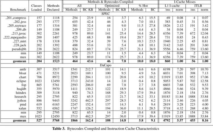
To measure the complexity of the benchmark code, we use the Chi-damber and Kemerer object-oriented programming (CK) metrics [12] measured with the ckjm software package [36]. We apply the CK metrics to classes that the application actually loads during exe-cution. We exclude standard libraries from this analysis as they are heavily duplicated across the benchmarks (column two of Table 3 includes all loaded classes). The average DaCapo program loads more than twice as many classes during execution as SPEC. The following explains what the CK metrics reveal and the results for SPEC and DaCapo.

WMC Weighted methods per class. Since ckjm uses a weight

of 1, WMC is simply the total number of declared methods for the loaded classes. Larger numbers show that a program provides more behaviors, and we see SPEC has substantially lower WMC values than DaCapo, except for 213 javac, which as the table shows is the richest of the SPEC benchmarks and usually falls in the middle or top of the DaCapo’s program range of software complexity. Unsurprisingly, fewer methods are declared (WMC in Table 2) than compiled (Table 3), but this difference is only dramatic for eclipse.

DIT Depth of Inheritance Tree. DIT provides for each class a

measure of the inheritance levels from the object hierarchy top. In Java where all classes inherit Object the minimum value of DIT is 1. Except for 213 javac and 202 jess, DaCapo programs typically have deeper inheritance trees.

NOC Number of Children. NOC is the number of immediate

subclasses of the class. Table 2 shows that in SPEC, only

213 javac has any interesting behavior, but hsqldb, luindex, lusearch and pmd in DaCapo also have no superclass structure.

CBO Coupling between object classes. CBO represents the

num-ber of classes coupled to a given class (efferent couplings). Method calls, field accesses, inheritance, arguments, return types, and exceptions all couple classes. The interactions be-tween objects and classes is substantially more complex for

Benchmark WMC DIT NOC CBO RFC LCOM

SPEC 201 compress 154 19 0 55 426 780 202 jess 614 97 1 632 1846 2032 205 raytrace 330 33 3 117 743 1046 209 db 152 12 0 42 454 789 213 javac 1011 186 38 1175 3293 3753 222 mpegaudio 367 40 0 167 796 1350 227 mtrt 332 33 3 117 743 1046 228 jack 375 46 0 163 860 6911 pseudojbb 541 35 0 254 1419 2487 min 152 12 0 42 426 780 max 1011 186 38 1175 3293 6911 geomean 366 40 2 176 950 1701 DaCapo antlr 1253 84 8 674 3094 8444 bloat 2265 206 21 1661 6232 6521 chart 1627 101 16 648 3979 29169 eclipse 10763 830 164 7277 26209 218199 fop 1433 148 17 998 3867 13041 hsqldb 2419 73 3 766 4676 47371 jython 3023 225 60 1398 5725 97111 luindex 494 50 0 246 1372 2260 lusearch 618 55 0 297 1441 3419 pmd 2348 215 4 1199 5384 126893 xalan 2433 161 24 971 5682 37394 min 494 50 0 246 1372 2260 max 10763 830 164 7277 26209 218199 geomean 1857 138 10 935 4420 22561

WMC Weighted methods/class CBO Object class coupling DIT Depth Inheritance Tree RFC Response for a Class NOC Number of Children LCOM Lack of method cohesion

Table 2. CK Metrics for Loaded Classes (Excluding Libraries)

DaCapo compared to SPEC. However, both 202 jess and 213 javac have relatively high CBO values.

RFC Response for a Class. RFC measures the number of different

methods that may execute when a method is invoked. Ideally, we would find for each method of the class, the methods that class will call, and repeat for each called method, calculating the transitive closure of the method’s call graph. Ckjm calcu-lates a rough approximation to the response set by inspecting method calls within the class’s method bodies. The RFC metric for DaCapo shows a factor of around five increase in complex-ity over SPEC.

LCOM Lack of cohesion in methods. LCOM counts methods in

a class that are not related through the sharing of some of the class’s fields. The original definition of this metric (used in ckjm) considers all pairs of a class’s methods, subtracting the number of method pairs that share a field access from the number of method pairs that do not. Again, DaCapo is more complex, e.g., eclipse and pmd have LCOM metrics at least two orders of magnitude higher than any SPEC benchmark. In summary, the CK metrics show that SPEC programs are not very object-oriented in absolute terms, and that the DaCapo benchmarks are significantly richer and more complex than SPEC. Furthermore, DaCapo benchmarks extensively use object-oriented features to manage their complexity.

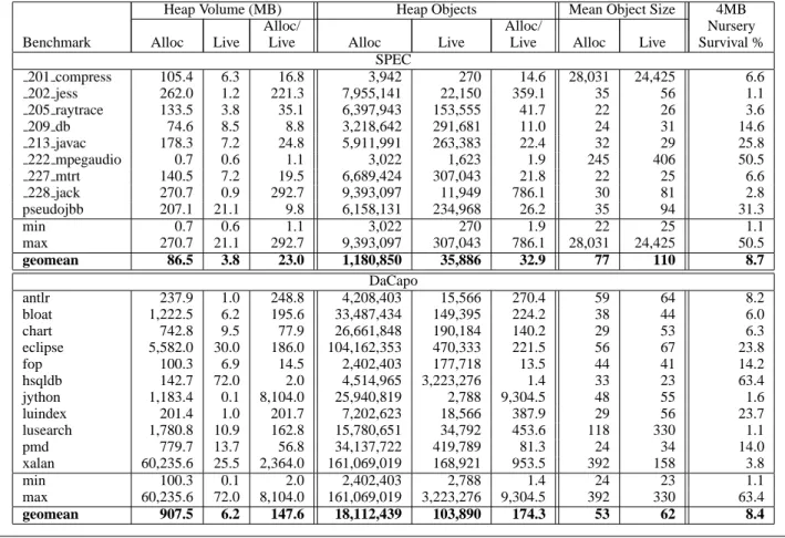
6.2 Code Size and Instruction Cache Performance

This section presents program size metrics. Column 2 of Table 3 shows the total number of classes loaded during the execution of each benchmark, including standard libraries. Column 3 shows the total number of declared methods in the loaded classes (compare to column 2 of Table 2, which excludes standard libraries). Columns 4 and 5 show the number of methods compiled (executed at least

Methods & Bytecodes Compiled I-Cache Misses

Classes Methods All Optimized % Hot L1 I-cache ITLB

Benchmark Loaded Declared Methods BC KB Methods BC KB Methods BC /ms norm /ms norm SPEC 201 compress 157 1118 254 23.9 16 3.7 6.3 15.5 69 0.08 4 0.07 202 jess 293 1777 655 42.4 46 4.3 7.0 10.1 383 0.45 31 0.56 205 raytrace 177 1316 381 32.4 44 9.0 11.5 27.8 1826 2.12 191 3.42 209 db 149 1108 249 23.7 11 1.5 4.4 6.3 34 0.04 2 0.04 213 javac 302 2261 978 89.0 141 25.4 14.4 28.5 6356 7.39 672 12.04 222 mpegaudio 200 1407 425 68.3 88 19.4 20.7 28.4 731 0.85 24 0.43 227 mtrt 178 1318 379 32.4 39 7.6 10.3 23.5 1940 2.25 45 0.81 228 jack 202 1392 488 53.6 33 5.4 6.8 10.1 3142 3.65 201 3.60 pseudojbb 238 2622 824 69.7 174 25.7 21.1 36.9 5556 6.46 759 13.60 min 149 1108 249 23.7 11 1.5 4.4 6.3 34 0.04 2 0.04 max 302 2622 978 89.0 174 25.7 21.1 36.9 6356 7.39 759 13.60 geomean 204 1523 464 43.6 46 7.8 10.0 18.0 860 1.00 56 1.00 DaCapo antlr 307 3517 1541 212.7 101 14.1 6.6 6.6 6198 7.20 597 10.70 bloat 471 5231 2023 169.1 100 9.5 4.9 5.6 6031 7.01 398 7.13 chart 706 8972 2299 204.1 113 20.8 4.9 10.2 11919 13.85 952 17.06 eclipse 1023 12450 3713 243.0 14 2.0 0.4 0.8 5053 5.87 702 12.58 fop 865 5761 2593 206.0 69 7.8 2.7 3.8 6603 7.68 532 9.53 hsqldb 355 5970 1411 130.2 122 18.9 8.6 14.5 4866 5.66 524 9.39 luindex 309 3118 940 74.3 168 29.3 17.9 39.4 1876 2.18 154 2.76 lusearch 295 2795 822 65.5 133 21.7 16.2 33.1 10183 11.84 1888 33.84 jython 886 9443 3242 462.5 297 28.5 9.2 6.2 2114 2.46 226 4.05 pmd 619 6163 2247 152.4 137 14.3 6.1 9.4 2819 3.28 223 4.00 xalan 552 6562 1747 126.2 194 36.0 11.1 28.5 3718 4.32 268 4.80 min 295 2795 822 65.5 14 2.0 0.4 0.8 1876 2.18 154 2.76 max 1023 12450 3713 462.5 297 36.0 17.9 39.4 11919 13.85 1888 33.84 geomean 527 5768 1866 162.4 108 14.8 5.8 9.1 4792 5.57 455 8.16

Table 3. Bytecodes Compiled and Instruction Cache Characteristics

once) and the corresponding KB of bytecodes (BC KB) for each benchmark. We count bytecodes rather than machine code, as it is not virtual machine, compiler, or ISA specific. The DaCapo bench-marks average more than twice the number of classes, three times as many declared methods, four times as many compiled methods, and four times the volume of compiled bytecodes, reflecting a sub-stantially larger code base than SPEC. Columns 6 and 7 show how much code is optimized by the JVM’s adaptive compiler over the course of two iterations of each benchmark (which Eeckhout et al.’s results indicate is probably representative of most hotspot finding virtual machines [19]). Columns 8 and 9 show that the DaCapo benchmarks have a much lower proportion of methods which the adaptive compiler regards as hot. Since the virtual machine selects these methods based on frequency thresholds, and these thresholds are tuned for SPEC, it may be that the compiler should be selecting warm code. However, it may simply reflect the complexity of the benchmarks. For example, eclipse has nearly four thousand meth-ods compiled, of which only 14 are regarded as hot (0.4%). On the whole, this data shows that the DaCapo benchmarks are sub-stantially larger than SPEC. Combined with their complexity, they should present more challenging optimization problems.

We also measure instruction cache misses per millisecond as another indicator of dynamic code complexity. We measure misses with the performance counters on a 2.0 GHz Pentium M with a 32KB level 1 instruction cache and a 2MB shared level two cache, each of which are 8-way with 64 byte lines. We use Jikes RVM and only report misses during the mutator portion of the second iteration of the benchmarks (i.e., we exclude garbage collection). Columns 10 and 11 show L1 instruction misses, first as misses per millisecond, and then normalized against the geometric mean of the SPEC benchmarks. Columns 12 and 13 show ITLB misses using the same metrics. We can see that on average DaCapo has L1 I-cache misses nearly six times more frequently than SPEC, and ITLB misses about eight times more frequently than SPEC. In

particular, none of the DaCapo benchmarks have remarkably few misses, whereas SPEC benchmarks 201 compress, 202 jess, and

209 db hardly ever miss the IL1. All DaCapo benchmarks have

misses at least twice that of the geometric mean of SPEC.

7.

Objects and Their Memory Behavior

This section presents object allocation, live object, lifetime, and lifetime time-series metrics. We measure allocation demographics suggested by Dieckmann and H¨olzle [15]. We also measure lifetime and live object metrics, and show that they differ substantially from allocation behaviors. Since many garbage collection algorithms are most concerned with live object behaviors, these demographics are more indicative for designers of new collection mechanisms. Other features, such as the design of per-object metadata, also depend on the demographics of live objects, rather than allocated objects.

The data described in this section and Section 8 is presented in Table 4, and in Figures 4(a) through 22(a), each of which contains data for one of the DaCapo or SPEC benchmarks. Each figure includes a brief description of the benchmark, key attributes, and metrics. It also plots time series and summaries for (a) object size demographics (Section 7.2), (b) heap composition (Section 7.3), and (c) pointer distances (Section 8). Together this data shows that the DaCapo suite has rich and diverse object lifetime behaviors.

Since Jikes RVM is written in Java, the execution of the JIT compiler normally contributes to the heap, unlike most other JVMs, where the JIT is written in C. In these results, we exclude the JIT compiler and other VM objects by placing then into a separate, excluded heap. To compute the average and time-series object data, we modify Jikes RVM to keep statistics about allocations and to compute statistics about live objects at frequent snapshots, i.e., during full heap collections.

7.1 Allocation and Live Object Behaviors

Table 4 summarizes object allocation, maximum live objects, and their ratios in MB (megabytes) and objects. The table shows that

Heap Volume (MB) Heap Objects Mean Object Size 4MB

Alloc/ Alloc/ Nursery

Benchmark Alloc Live Live Alloc Live Live Alloc Live Survival %

SPEC 201 compress 105.4 6.3 16.8 3,942 270 14.6 28,031 24,425 6.6 202 jess 262.0 1.2 221.3 7,955,141 22,150 359.1 35 56 1.1 205 raytrace 133.5 3.8 35.1 6,397,943 153,555 41.7 22 26 3.6 209 db 74.6 8.5 8.8 3,218,642 291,681 11.0 24 31 14.6 213 javac 178.3 7.2 24.8 5,911,991 263,383 22.4 32 29 25.8 222 mpegaudio 0.7 0.6 1.1 3,022 1,623 1.9 245 406 50.5 227 mtrt 140.5 7.2 19.5 6,689,424 307,043 21.8 22 25 6.6 228 jack 270.7 0.9 292.7 9,393,097 11,949 786.1 30 81 2.8 pseudojbb 207.1 21.1 9.8 6,158,131 234,968 26.2 35 94 31.3 min 0.7 0.6 1.1 3,022 270 1.9 22 25 1.1 max 270.7 21.1 292.7 9,393,097 307,043 786.1 28,031 24,425 50.5 geomean 86.5 3.8 23.0 1,180,850 35,886 32.9 77 110 8.7 DaCapo antlr 237.9 1.0 248.8 4,208,403 15,566 270.4 59 64 8.2 bloat 1,222.5 6.2 195.6 33,487,434 149,395 224.2 38 44 6.0 chart 742.8 9.5 77.9 26,661,848 190,184 140.2 29 53 6.3 eclipse 5,582.0 30.0 186.0 104,162,353 470,333 221.5 56 67 23.8 fop 100.3 6.9 14.5 2,402,403 177,718 13.5 44 41 14.2 hsqldb 142.7 72.0 2.0 4,514,965 3,223,276 1.4 33 23 63.4 jython 1,183.4 0.1 8,104.0 25,940,819 2,788 9,304.5 48 55 1.6 luindex 201.4 1.0 201.7 7,202,623 18,566 387.9 29 56 23.7 lusearch 1,780.8 10.9 162.8 15,780,651 34,792 453.6 118 330 1.1 pmd 779.7 13.7 56.8 34,137,722 419,789 81.3 24 34 14.0 xalan 60,235.6 25.5 2,364.0 161,069,019 168,921 953.5 392 158 3.8 min 100.3 0.1 2.0 2,402,403 2,788 1.4 24 23 1.1 max 60,235.6 72.0 8,104.0 161,069,019 3,223,276 9,304.5 392 330 63.4 geomean 907.5 6.2 147.6 18,112,439 103,890 174.3 53 62 8.4

Table 4. Key Object Demographic Metrics

DaCapo allocates substantially more objects than the SPEC bench-marks, by nearly a factor of 20 on average. The live objects and memory are more comparable; but still DaCapo has on average three times the live size of SPEC. DaCapo has a much higher ratio of allocation to maximum live size, with an average of 147 com-pared to SPEC’s 23 measured in MB. Two programs stand out;

jython with a ratio of 8104, and xalan with a ratio of 2364. The

DaCapo benchmarks therefore put significantly more pressure on the underlying memory management policies than SPEC.

Nursery survival rate is a rough measure of how closely a pro-gram follows the generational hypothesis which we measure with respect to a 4MB bounded nursery and report in the last column of Table 4. Note that nursery survival needs to be viewed in the context of heap turnover (column seven of Table 4). A low nurs-ery survival rate may suggest low total GC workload, for exam-ple, 222 mpegaudio and hsqldb in Table 4. A low nursery survival rate and a high heap turnover ratio instead suggests a substantial GC workload, for example, eclipse and luindex. SPEC and Da-Capo exhibit a wide range of nursery survival rates. Blackburn et al. show that even programs with high nursery survival rates and large turnover benefit from generational collection with a copying bump-pointer nursery space [4]. For example, 213 javac has a nursery survival rate of 26% and performs better with generational collec-tors. We confirm this result for all the DaCapo benchmarks, even on hsqldb with its 63% nursery survival rate and low turnover ratio. Table 4 also shows the average object size. The benchmark suites do not substantially differ with respect to this metric. A sig-nificant outlier is 201 compress, which compresses large arrays of data. Other outliers include 222 mpegaudio, lusearch and xalan, all of which also operate over large arrays.

7.2 Object Size Demographics

This section improves the above methodology for measuring object size demographics. We show that these demographics vary with time and when viewed from of perspective of allocated versus live objects. Allocation-time size demographics inform the structure of the allocator. Live object size demographics impact the design of per-object metadata and elements of the garbage collection algo-rithm, as well as influencing the structure of the allocator. Fig-ures 4(a) through 22(a) each use four graphs to compare size de-mographics for each DaCapo and SPEC benchmark. The object size demographics are measured both as a function of all alloca-tions (top) and as a function of live objects seen at heap snapshots (bottom). In each case, we show both a histogram (left) and a time-series (right).

The allocation histogram plots the number of objects on the y-axis in each object size (x-axis in log scale) that the program allocates. The live histogram plots the average number of live objects of each size over the entire program. We color every fifth bar black to help the eye correlate between the allocation and live histograms. Consider antlr in Figure 4(a) and bloat in Figure 5(a). For antlr, the allocated versus live objects in a size class show only modest differences in proportions. For bloat however, 12% of its allocated objects are 38 bytes whereas essentially no live objects are 38 bytes, which indicates they are short lived. On the other hand, less than 1% of bloat’s allocated objects are 52 bytes, but they make up 20% of live objects, indicating they are long lived. Figure 14(a) shows that for xalan there is an even more marked difference in allocated and live objects, where 50% of allocated objects are 12 bytes, but none stay live. In fact, 65% of live objects are 2 Kbytes, whereas they make up only 2% of allocated objects.

How well these large objects are handled will thus in large part determine the performance of the collector on xalan.

For each allocation histogram, we also present a time series graph in Figures 4(a) through 22(a).. Each line in the time series graph represents an object size class from the histogram on the left. We color every fifth object size black, stack them, and place the smallest size classes at the bottom of the graphs. The distance between the lines indicates the cumulative number of objects allo-cated or live of the corresponding size, as a function of time (in bytes of allocation by convention).

Together, the histogram and time-series data show marked dif-ferences between allocated and live object demographics. For ex-ample, the allocation histograms for bloat, fop, and xalan (Fig-ures 5(a), 8(a), 14(a)) are similar, but the time series data shows many differences. The xalan program has eight allocation phases that are self-similar and mirrored in the live data, although in dif-ferent size class proportions. Whereas, in bloat allocation and live objects show much less phase behavior, and phases are not self-correlated. Comparing live and allocated time-series for fop shows a different pattern. There is a steady increase in the live objects of each size (and consequently, probably growing data structures), whereas fop allocates numerous sizes in a several distinct allocation phases. Thus, the allocation and live graphs are very different. This shows that live and allocation time series analysis can reveal com-plexity and opportunities that a scalar metric will never capture.

7.3 Heap Composition Graphs

Figures 4(b) through 22(b) each plot heap composition in lines of constant allocation as a function of time, measured in allocations (top) and pointer mutations (bottom). Like the live object time series graphs, these graphs expose the heap composition but show object lifetime behaviors rather than object size. Since both graphs show live objects, their shapes are similar. The heap composition graphs group objects into cohorts based on allocation time. We choose cohort sizes as a power of two (2n_{) such that there are} between 100 and 200 cohorts, shown as a line in each graph. The top line corresponds to the oldest cohort and indicates the total volume of live objects in the heap. The gaps between each of the lines reflects the amount in each cohort, and when objects in a cohort die, adjacent lines move closer together or if they all die, the lines merge. It is not uncommon for programs to immediately allocate long lived data, indicated by a gap between the top line and the other cohorts; bloat, hsqldb, jython, and lusearch all show this behavior in Figures 5(b), 9(b), 10(b), and 12(b).

Qualitatively, the complexity of the graphs in Figures 4(b) through 22(b) reflect the object lifetime behaviors of each of the benchmarks. With the exception of jython and lusearch, the Da-Capo benchmarks show much richer lifetime behaviors than SPEC;

jython is an interpreter, which leads to a highly regular

execu-tion pattern. Although jython allocates more than any of the SPEC benchmarks, its behavior is highly regular. We experimented with a number of interpreted workloads and found very similar, highly regular behavior, suggesting that the interpreter rather than the in-terpreted program dominates. The programs chart and xalan show distinct self-similar phases with respect to object lifetimes in Fig-ures 6(b) and and 14(b). The programs fop and hsqldb show regu-lar, steady heap growth in Figures 8(b) and 9(b). On the other hand,

bloat, eclipse, luindex, and pmd show irregular, complex object

lifetime patterns in Figures 5(b), 7(b), 11(b), and 13(b).

8.

Reference Behavior in Pointer Distances

Java programs primarily use pointer-based data structures. This section provides statistics that describe the connectivity of the data structures created and manipulated by the DaCapo and SPEC benchmarks. We measure pointer distance between its source and target objects by the relative ages of the objects, for both static

snapshots of the heap, and dynamically as pointers change. These properties influence aspects of memory performance, such as tem-poral and spatial locality and the efficacy of generational garbage collectors.

Figures 4(c) through 22(c) show the relative distances between the sources and targets of pointers in the heap for each benchmark. Pointer distance is measured by the difference between the target and source object positions within (a close approximation to) a per-fectly compacted heap. We approximate a continuously perper-fectly compacted heap by tracking cohort sizes and the logical position of each object within each cohort during frequent garbage collec-tions. The youngest object has a heap position of 0 and the oldest has a heap position equal to the volume of live objects in the heap. Thus, positive values are old to young object pointers, and negative values are young to old.

We include both a ‘static’ snapshot measure of pointer distance, and a ‘dynamic’ mutation measure. Snapshot pointer distance is established by examining all pointers in the live object graph at a garbage collection–measuring the state of the object graph. Mu-tation distance is established by examining every pointer as it is created–measuring the activity over the object graph. We express these metrics as aggregate histograms for the execution of the en-tire benchmark, and as a time series to reflect the changing shape of the histogram over time (measured in mutations).

We first consider snapshot pointer distance, the top histogram and time series in Figures 4(c) through 22(c). The most striking feature of these graphs is the wide range of behaviors displayed by the benchmarks. Several programs show very irregular time-varying behavior, e.g., antlr, chart, eclipse, and luindex; whereas

bloat hsqldb, and pmd are more stable, but still vary a bit; and xalan

shows a very complex, but exactly repeated pattern. Several of the SPEC benchmarks, such as 202 jess, 205 raytrace, and 209 db display a completely flat pointer distance profile.

The mutation pointer distance graphs have the same axes and are shown below each snapshot pointer distance figure. These graphs are computed by tracking pointer distances at all pointer stores (in a write barrier), rather than at static snapshots of the heap. These graphs show a wider range of irregularity and patterns than the heap snapshots.

To illustrate the differences between these metrics, consider

bloat in Figure 5(c). Many pointers point from old to new objects

(positive numbers in the snapshot graphs in the top half of Fig-ure: 5(c)), but almost all pointer mutations install new to old point-ers (negative numbpoint-ers in the mutation graphs). The snapshot graphs indicate that around 40% of pointers will point from old to new at any given snapshot (see the top-most line in the time series) and about 60% will point from new to old (the bottom-most line). On the other hand, the mutation graphs show that for most of the execu-tion of the benchmark, nearly 100% of pointer mutaexecu-tions are in the new to old direction. The divergence of the snapshot and mutation data, and the time-varying nature of each highlight the limitations of single value summaries of benchmark behaviors.

9.

Principal Components Analysis

Previous sections demonstrate that DaCapo is more object oriented, more complex, and larger than SPEC, whereas this section demon-strates that all the constituent programs differ from each other, us-ing principal component analysis (PCA) [18]. This result indicates that we satisfy our goal of program diversity. It also confirms that DaCapo benchmarks differ from SPEC, which is unsurprising by now given the results from the preceding sections.

PCA is a multivariate statistical technique that reduces a large

N dimensional space into a lower dimensional uncorrelated space.

PCA generates a positive or negative weight (factor loading) associ-ated with each metric. These weights transform the original higher dimension space into P principal components using linear

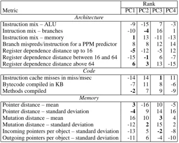
equa-Rank

Metric PC1 PC2 PC3 PC4

Architecture

Instruction mix – ALU -9 -15 7 -3

Intruction mix – branches -10 -4 16 1

Instruction mix – memory 1 13 -11 -13

Branch mispreds/instruction for a PPM predictor 8 8 12 14 Register dependence distance up to 16 -5 -12 -5 12 Register dependence distance between 16 and 64 -15 -1 6 -7 Register dependence distance above 64 6 3 13 -15

Code

Instruction cache misses in miss/msec -14 14 1 11

Bytecode compiled in KB -7 11 8 -6

Methods compiled -2 7 9 -9

Memory

Pointer distance – mean 3 -16 10 -5

Pointer distance – standard deviation -4 9 14 16

Mutation distance – mean 16 10 3 4

Mutation distance – standard deviation -12 2 15 2 Incoming pointers per object – standard deviation -13 5 -2 -8 Outgoing pointers per object – standard deviation -11 6 -4 -10

Table 5. Metrics Used for PC Analysis and Their PC Rankings

tions. We follow the PCA methodology from prior work [13, 19], but use different constituent metrics. Table 5 shows these metrics which cover architecture, code, and memory behavior. We include architecture metrics to expand over the code and memory met-rics presented and explored in depth by previous sections, and to see which of these differentiate the benchmarks. Our code met-rics include the i-cache miss rate for each benchmark, the number of methods compiled and the volume of bytecodes compiled. The

memory metrics include static and dynamic pointer distances, and

incoming and outgoing pointer distributions.

Following prior work [27], our architecture metrics are micro-architecture neutral, meaning that they capture key architectural characteristics such as instruction mix, branch prediction, and register dependencies, but do so independently of the underlying micro-architecture. We gather these metrics using a modified ver-sion of Simics v. 3.0.11 [42]. We use our harness to measure stable performance in Sun’s HotSpot JVM, v. 1.5.0 07-b03 running on a simulated Sun Ultra-5 10 with Solaris 9.

PCA computes four principal components (PC1, PC2, PC3, and PC4) which in our case account for 70% of the variance between benchmarks. PCA identifies principal components in order of sig-nificance; PC1 is the most determinative component and PC4 is the least. Table 5 shows the relative ranks of each of the metrics for PC1–PC4. The absolute value of the numbers in columns 2–5 in-dicates the rank significance of the metric, while the sign inin-dicates whether the contribution is negative or positive. We bold the ten most significant values overall; six of these contribute to PC1, four to PC2, three to PC3, and none to PC4. Memory instruction mix is the most significant metric for PC1, and methods compiled is the next most significant. Note that the three most significant contribu-tors to PC1 cover each of the three metric categories.

Scatter plots in Figure 3 show how the benchmarks differ in two-dimensional space. Figure 3 plots each program’s PC1 value against its PC2 value in the top graph, and Figure 3 plots PC3 and PC4 in the bottom graph. Intuitively, the further the distance between two benchmarks, the further apart they are with respect to the metrics. The benchmarks differ if they are apart in either graph. Since the programs are well distributed in these graphs, the benchmarks differ.

10.

Conclusion

Benchmarks play a strategic role in computer science research and development by creating a common ground for evaluating ideas and products. The choice of benchmarks and benchmarking

- 1 . 5 - 1 . 0 - 0 . 5 0 . 0 0 . 5 1 . 0 1 . 5 2 . 0 2 . 5 Component 1 - 1 . 5 - 1 . 0 - 0 . 5 0 . 0 0 . 5 1 . 0 1 . 5 2 . 0 2 . 5 3 . 0 Component 2 xalan p m d lusearch luindex jython hsqldb f o p eclipse chart bloat antlr jack m t r t mpegaudio javac d b raytrace jess compress - 1 0 1 2 Component 3 - 2 . 0 0 - 1 . 7 5 - 1 . 5 0 - 1 . 2 5 - 1 . 0 0 - 0 . 7 5 - 0 . 5 0 - 0 . 2 5 0.00 0.25 0.50 0.75 1.00 1.25 1.50 1.75 Component 4 xalan p m d lusearch luindex jython hsqldb f o p eclipse chart bloat antlr jack m t r t mpegaudio javac d b raytrace jess compress

Figure 3. PCA Scatter Plots; PC1 & PC2 (top), and PC3 & PC4.

methodology can therefore have a significant impact on a research field, potentially accelerating, retarding, or misdirecting energy and innovation. Prompted by concerns among ourselves and others about the state-of-the-art, we spent thousands of hours at eight separate institutions examining and addressing the problems of benchmarking Java applications. The magnitude of the effort surely explains why so few have developed benchmark suites.

This paper makes two main contributions: 1) it describes a range of methodologies for evaluating Java, including a number of new analyses, and 2) it presents the DaCapo benchmark suite. We show that good methodology is essential to drawing meaningful conclu-sions and highlight inadequacies prevalent in current methodology. A few of our specific methodology recommendations are:

• When selecting benchmarks for a suite, use PCA to quantify benchmark differences with metrics that include static and dy-namic code and data behavior.

• _{When evaluating architectures use multiple JVMs. Evaluating}

new architecture features will also benefit from multiple JVMs.

• When evaluating JVM performance, use multiple architectures with mix and stable methodologies, reporting first and/or sec-ond iterations as well as steady-state to explore the compile and runtime tradeoffs in the JVM.

• When measuring memory performance, use and report heap sizes proportional to the minimums.

• _{When measuring GC and JIT compilation performance use mix}

and stable methodologies, and use constant workload (rather than throughput) benchmarks.

• When measuring GC or compile time overheads use determin-istic stable and mix methodologies.

This paper uses these methodologies to demonstrate that the Da-Capo benchmarks are larger, more complex and richer than the commonly used SPEC Java benchmarks. The DaCapo benchmarks