Real exchange rate and productivity in China

Document de travail de la série Etudes et Documents

Ec 2003.28

Real exchange rate and productivity in China

Sylviane GUILLAUMONT JEANNENEY

*1

and Ping HUA

*

CERDI-IDREC, CNRS-Université d’Auvergne 65, boulevard François Mitterrand,

63000 Clermont-Ferrand, France. Tel: 33 4 73 17 74 05 Fax: 33 4 73 17 74 28

Email: S.Guillaumont@u-clermont1.fr, P.Hua@u-clermont1.fr.

octobre 2003 37 p.

1

The corresponding author: Sylviane Guillaumont-Jeanneney, CERDI, 65 Boulevard François Mitterrand, 63000 Clermont-Ferrand, France. Tel: 00 33 4 73 17 74 05, Fax: 00 33 4 73 17 74 28, Email: S.Guillaumont@u-clermont1.fr.

*

The authors would thank Laurent Cortèse for his technical help about DEA Malmquist Index calculation and Martine Bouchut for real effective exchange rate calculation.

Real exchange rate and productivity in China

Sylviane Guillaumont Jeanneney and Ping Hua

Summary

This article investigates the impact that the real exchange rate appreciation in China has exerted on productivity growth since 1994. We remind the arguments explaining a positive or a negative impact of a real appreciation on efficiency and on technical progress. DEA Malmquist indices of productivity growth and of its two components are calculated for twenty-nine Chinese provinces. The econometric estimation shows that the appreciation of the real exchange rate had an unfavourable effect on technical progress but a favourable effect on efficiency growth, and these two effects offset each other partially to give a lesser negative effect on productivity growth.

Key words: China, DEA Malmquist index, productivity, real exchange rate.

Résumé

Cet article étudie l’impact que l’appréciation du taux de change réel en Chine entre 1993 et 2001 a exercé sur la croissance de la productivité globale des facteurs de production.. On expose les arguments susceptibles d’expliquer un impact positif ou négatif sur l’efficience technique et sur le progrès technique Puis, grâce à un indice de Malmquist calculé avec la méthode DEA, on décompose la croissance de la productivité entre ses deux composantes pour l’ensemble des provinces chinoises . Enfin on présente une estimation en panel de la croissance de la productivité des facteurs et l’on montre que l’appréciation du taux de change réel a exercé une action défavorable sur le progrès technique en partie compensée par une action favorable sur la croissance de l’efficience.

1 Introduction

Industrialized countries have experienced large fluctuations of real exchange rates

during the last thirty years so that many authors have taken an interest in the link between the

level of real exchange rates and productivity growth in these economies. So Paul Krugman

(1989) suggested that the large appreciation of the dollar between 1979 and 1985 might have

induced the acceleration of industrial productivity growth in the United-States because the

rise of the dollar would have pushed firms to increase their productivity. In the same way

Porter (1990), in his well-known book about competitiveness and growth, upheld that an

overvalued exchange rate might contribute to increase productivity. Inversely it is likely that

the large real depreciation of the Canadian dollar during the 1990’s explains the widening

productivity gap between the United-States and Canada (Courchene and Harris, 1999, Grubel,

1999).

However for developing countries one does not generally make the hypothesis that a

real appreciation of one currency has a positive impact on productivity. Most authors think

that an overvaluation of currency, by reducing the competitiveness of tradable goods sector,

affects negatively productivity growth

2

. China is a very appropriate field to investigate the

effects of an appreciation of the real exchange rate on productivity growth. Indeed since the

beginning of the last decade China has really become a market economy (Guillaumont and

Hua, 2002). In 1992, a break in the reforms, the process of liberalization and trade openness is

launched again, following the famous trip of Deng Xiaoping in the South of China. At this

time there were still two exchange rates for the dollar in terms of Renminbi for commercial

operations, an official rate and a higher swap rate which was determined on foreign exchange

markets but was strictly controlled by the central rulers. The firms should sell 20% of their

exports receipts at the official rate and might use the remaining 80% to finance their own

2

An exception is Lu and Qiao (1999) who assume a positive relationship between the appreciation of the real exchange rate and productivity growth in Singapore.

imports or sell them on the foreign exchange markets at the swap rate. The planned imports

were supported by priority foreign allowances at the official rate while the other imports were

financed at the swap rate. However, since the beginning of 1994, only swap rate exists. While

previously the two exchange rates were periodically devalued, the rate of exchange of the

Renminbi in terms of dollar, henceforth the only remaining one, has remained constant.

Therefore the real effective exchange rate of China, which was strongly depreciated in 1992

and 1993, has known some appreciation until 1998 and then a stabilization (see Figure 1)

3

(Guillaumont Jeanneney and Hua, 2001). The real appreciation of the Chinese currency did

not prevent the economy from growing at a rate which has been permanently higher than 7%

per annum.

Moreover, the variation of the real exchange rate differs from one province to one

another because the provinces have very different rates of inflation as well as different foreign

trading partners (Guillaumont Jeanneney and Hua, 2002). From 1993 to 2001, the annual

average appreciation of the real effective exchange rates of Chinese provinces has ranged

from 2.6 in Hainan to 6.6 in Beijing municipality (see figure 2).

4

Figure 1

0 20 40 60 80 100 120 140 1991 1992 1993 1994 1995 1996 1997 1998 1999 2000 2001

NB .A rise means an appreciation of the Renminbi.

3

The calculation of the real effective exchange rate is explicated below in the section 4.1

4

The rates of appreciation are calculated on the base of the price of the Renminbi in terms of foreign currencies, namely on the base of the ratio of consumer prices in China expressed in foreign currencies to consumer prices in foreign countries.

It would not be convenient to measure the impact of the real exchange rate on factor

productivity without taking in account the reverse effect of productivity on growth, stated by

Balassa (1964) and Samuelson (1964). These authors have shown that real exchange rate

tends to appreciate in countries where productivity growth (which occurs chiefly in the

tradable goods sector) is faster than in the rest of the world. Indeed, “under the assumption

that prices equal marginal costs, inter-country wages differences in the sector of tradable

goods will correspond to productivity differentials, while the internal mobility of labor will

tend to equalize the wages of comparable labor within each economy” (Balassa, 1964, p.586).

So the growth of productivity tends to raise the price of non-tradable goods domestically

determined. Regarding Chinese provinces as different economies, we have shown elsewhere

(Guillaumont Jeanneney and Hua, 2002) that, in the long run, the differences between the real

exchange rates of Chinese provinces may be explained by the Balassa-Samuelson effect. This

effect is captured by the gap between the per capita product of each province and respectively

that of its foreign trading partners and that of China as a whole.

5

In the following econometric

estimation of the impact of the real exchange rate on productivity growth, we shall use these

gaps as instruments for the real exchange rate.

Figure 2

0 1 2 3 4 5 6 7 Hainan

Guizhou Guangxi Fujian

Hebei

Ningxia Hubei _Xinjiang Jiangsu Anhui _Liaoning Shanxi Hunan

Shandong

Beijing

5

Indeed one province trades with foreign countries and with other Chinese provinces, what justifies these two gaps..

This paper is organized as follows. In part 2 we present theoretical assumptions, which

may justify a relationship between the level of the real exchange rate and the growth of

factors productivity and we set out their empirical counterparts. This analysis suggests that the

real exchange rate does not affect productivity through the same channels whether

productivity growth is due to efficiency improvement or technical progress. It is why in the

third part we decompose the productivity growth into its two components thanks to DEA

Malmquist indices (Data Envelopment Analysis). Then in the fourth part we present our

empirical results, based on an estimation using fixed effects on a panel data of 29 provinces

over the period 1993-2001. We estimate successively efficiency variation, technical progress

and total factors productivity growth as a function of real exchange rate, of intermediary

variables representing the main channels through which real exchange rate affects

productivity growth and some other control variables. The results corroborate our assumption

that the real appreciation exerts a positive effect on efficiency growth, but a negative one on

technological change.

2. How does the appreciation

of the real exchange rate affect productivity growth: a

theoretical analysis

The literature presents opposite arguments about the effects of the real exchange rate on

total factor productivity, whether productivity growth is due to efficiency improvement or

technical progress. We remind the arguments which explain positive or negative impacts of

the appreciation of the real exchange rate, namely the fall of the relative price of tradable

goods, on productivity.

2.1. Why real appreciation should be good for productivity growth?

We may stress several reasons which support the idea that real appreciation is good for

productivity growth.

On the one hand, real appreciation decreases the relative cost of imported capital goods

and then induces a rise of the capital-labour ratio. It is likely that this rise supports technical

progress but simultaneously induces a lesser efficiency due to the drawbacks in the

management of more capitalistic and sophisticated technologies. On the other hand a real

appreciation means an increase in the real labour remuneration which may induce an

improvement of workers productivity particularly in a country where the wages of unskilled

workers are still very low. This assumption was presented as soon as 1957 by H. Leibenstein

who stressed that in developing countries a too weak remuneration of labour might spoil

workers’ health and their working capacity and showed that the motivation of workers acts on

efficiency, what he called the “X-efficiency”. However skilled workers are also concerned

with the increase of remunerations induced by a real appreciation of the exchange rate. We

may suppose that this last one slows down the emigration of this type of workers (Harris,

2001). In fact China endures a significant brain drain and in the 1990’s we observe some

Chinese workers coming back thanks to the improvement of skilled work remuneration

6

.

Finally it is likely that the real appreciation has exerted a positive effect on the

productivity of industrial enterprises in the extent that it has exacerbated foreign competition.

In the case of appreciation, firms may be compelled to close their less efficient factories. A

phenomenon of “creative destruction” benefits to the most efficient enterprises. It is also

possible that real appreciation pushes firms to improve their technical efficiency in a context

of monopoly or collusive oligopoly (Krugman, 1989). The argument is the following.

Managers benefit from only a part of the profit induced by a better management or a stronger

effort since a part of the profit goes to the owners of the enterprise. In the case of monopoly,

managers do not choose the exertion that maximises the profit. As Marshall said, the better

6

An appreciation may increase the return to skilled labour in a Stolper-Samuelson effect if the tradable sector is human-capital intensive relative to the non tradable sector (Harris, 2001, p.13)

profit of a monopoly is a quiet life. Then in a situation of oligopoly (due to the new foreign

competitors and, in the case of China, due to competitors localised in the other provinces) the

managers will choose a higher level of effort, not only because in the short run this behaviour

may increase their profit, but also because the decrease of costs dissuades competitors from

producing and thus avoids a fall in the price. Due to this strategic yield, there exists an

additional benefit induced by the effort which may push management effort nearer to its

optimum.

2.2. Why real appreciation should be deleterious to productivity growth?

The most current argument in favour of a harmful effect of the real exchange

appreciation on productivity growth is based on the fact that real appreciation tends to slow

down exports growth. Actually since the beginning of China’s transition towards a market

economy exports (in current dollars) have increased rapidly. However the annual export

growth has been slightly reduced during the 1990’s. It has passed from 13.7% on average

during the period 1985-1993, when the exchange rate depreciated, to 12.8% in 1994-2002,

when on the contrary the exchange rate appreciated. One expects that an increasing trade

openness exerts several kinds of favourable effects on productivity.

Export growth induces a shift of production factors into the export sector which is

generally considered as more efficient than the other sectors (Feder,1983; Guillaumont,

1994). This argument seems to be relevant for China where light industry of consumer goods

constitutes the bulk of the export sector (55% of exportations in 2001

7

). This productive

sector, very labour intensive, corresponds to the comparative advantage of China (Yue and

Hua, 2002) and technical efficiency is probably higher in this sector than in heavy industry or

in agriculture as well as in the service sector. This first argument is based on a dualistic view

of the economy according to which the labour marginal productivity is unequal in the

7

different sectors. This assumption seems to be relevant, as Chinese workers cannot freely

choose their work place. The relative advantage, in terms of efficiency, of the manufacturing

sector in China may have been progressively increased by the learning-by-doing effect and by

scale economies due to a market expansion. This advantage is probably still present several

years after the beginning of the transition of China towards a market economy and

consequently in the 1990’s. Indeed the export sector provides external economies to the whole

economy through the improvement of management skill and labour training.

On the other hand, the impact of the export sector on the technical progress is uncertain.

The industry of consumer goods or of small equipments, on which the export expansion is

based in China, is less capable to generate technical progress than the heavy industry, all the

more since a great part of this industry is only assembling of imported components.

Consequently, it is possible that an increasing ratio of exports to GDP would be associated

with a slow down in the technical progress.

The favourable effect of openness also passes through foreign direct investments

(Dayal-Gulati and Husain, 2002). In China, as in other developing countries, foreign

investments are concentrated in the sector of tradable goods, chiefly in industry. Until 1994

they have been stimulated by the real depreciation of the currency. Actually, as soon as 1993,

China became the country which received the most foreign direct investments among

developing countries (Démurger, 2002). Then, it is likely that the real appreciation would

have slowed down direct investments as it was observed in particular after the Asian crisis in

1997. One supposes that foreign firms bring in technological improvements and their

know-how

8

. This positive action occurs through the creation of subsidiary companies more

productive than domestic firms and through the diffusion of technical innovations and better

8

management in these firms. This imitation effect occurs in competing domestic firms, but still

more in firms which are suppliers or buyers of foreign enterprises (Sun, 1998).

However the negative potential effect of the appreciation of the real exchange rate on

productivity is not exclusively linked to a lesser growth of exports or of foreign direct

investments. Indeed real appreciation is a hindrance to import competing products as well as

exports. It reduces the profits and the capacity of self-financing, and therefore the investment

of the tradable goods sector (industry) for the benefit of services and protected sectors. If the

industrial sector is most innovative, real appreciation may slow down innovation well beyond

the only export industry or foreign enterprises.

In short, real exchange rate has many effects on total factor productivity which are

different whether productivity growth results from technical progress or from efficiency

improvement. A great part of these effects occurs through commercial and financial openness

which are hindered by a real appreciation. We expect a positive impact of trade openness

(measured by the export ratio) principally on efficiency while foreign direct investments

should be good for technical progress as well as for efficiency. On the other hand, real

appreciation, by rising capital labour intensity, should be favourable to technological

innovations, but unfavourable to efficiency. Moreover it is likely that the export ratio, the rate

of foreign direct investments and the capital-labour ratio do not capture all the effects of an

appreciation of the real effective exchange rate. This last one, corresponding to a relative fall

of tradable good prices, deters the investment in this most innovative part of the economy and

therefore is unfavourable to technical progress. In return real appreciation incites to improve

efficiency with a higher labour remuneration and an intensification of competition.

The effects of real appreciation that we have identified so far are long run phenomena

(Harris, 2001). In the short run, real appreciation may reduce the utilisation of production

capacity, by decreasing tradable goods demand and lead transitorily to a lesser efficiency.

2.3 Econometric model

As the expected effects of the real exchange rate are different on technical efficiency and progress, our econometric model distinguishes these two components of the productivity.

Consequently, three functions relative to technical efficiency change (TE• ), technical progress (TP• ), and total factor productivity growth (TFP• ) will be successively estimated. The sample is composed by the twenty-nine provinces of China over the period 1993-2001.

Among the explanatory variables, next to the real effective exchange rate (ER), we introduce several control variables, considered as independent of the real exchange rate, relative to the importance of public enterprises (ENP) and to the education level (EDU). Indeed we may suppose, as the essential of bank funding is affected to public enterprises in China, they make huge investments (with a high content of technological innovations) more easily than other enterprises, but in return their technical efficiency is constrained by an excess of workers difficult to be made redundant. On the other hand the presence of well-educated people is favorable to a good management and thus to an improvement of technical efficiency. Consequently, we introduced simultaneously three variables of human capital, concerning the proportion of the population having attained at best primary education level (EDUP), secondary education level (EDUS) or university education level (EDUU). Next to these variables of a structural nature, we introduced real GDP per capita lagged one period (YRP-1) to test an eventual convergence effect, following the traditional growth theory. In order to control for the transitory effect of business cycle on the utilization rate of production factors, we introduced the gap of the ratio between changes in inventories and GDP to its trend (INV) in the equation of technical efficiency and thus in the equation of total factor productivity growth. In fact, this ratio has met a decreasing trend during the estimated period which probably reflects a better efficiency in input utilization and in the management of finished goods, as this is normal in a transition economy. So we consider that a positive gap relative to trend reflects a flat overall economic situation and conversely a negative gap a booming one.

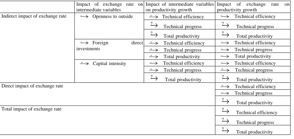
All the theoretical hypotheses relative to the effects of the real exchange rate presented before and the expected signs for the different variables which result from these hypotheses, are synthesized in table 1 where, as in our following estimation, an increase of the real exchange rate corresponds to a real appreciation. To test these hypotheses we carry out our estimation in three steps. At first we introduce the intermediate variables, identified as transmission channels of the real exchange rate to productivity change, namely the export rate (X), the foreign direct investments ratio (FDI) and capital intensity (KL). In this model the coefficient associated with the real exchange rate (ER) will capture the direct effects on productivity growth of the relative price change associated with a variation of the real exchange rate, effects that pass neither through export rate, nor through foreign direct investments, nor through capital intensity. We expect a negative coefficient for technical progress and a positive one for efficiency improvement.

Three functions can be therefore written as follows: For technical efficiency growth (equation 1):

it 10 it 9 it 8 it 7 1 it 6 it 5 it 4 it 3 it 2 it 1 0

it a aER a ENP aEDUP a EDUS a EDUU aYRP aINV aTX aFDI a KL

TE• = + + + + + + ₋+ + + +

The expected signs are such as:

a1>0, a2<0, a3<0, a4<0, a5>0, a6> or<0, a7<0, a8>0, a9>0, a10<0 For technical progress (equation 2):

it 9 it 8 it 7 1 it 6 it 5 it 4 it 3 it 2 it 1 0

it b bER bENP bEDUP b EDUS bEDUU bYRP bTX bFDI b KL

TP• = + + + + + + ₋+ + +

The expected signs are such as:

b1<0, b2>0, b3<0, b4<0, b5>0, b6> or<0, b7>or <0, b8>0, b9 >0 For total factor productivity growth (equation 3):

it 10 it 9 it 8 it 7 1 it 6 it 5 it 4 it 3 it 2 it 1 0

it c cER cENP cEDUP cEDUS cEDUU cYRP c INV cTX cFDI c KL

TFP• = + + + + + + ₋+ + + +

The expected signs are such as:

c1< or >0, c2< or>0, c3<0, c4<0, c5>0, c6>or<0, c7<0, c8<or>0, c9 >0, c10<or>0

Then, in order to measure the total effect of the real exchange rate on efficiency, technical progress and total factor productivity, we regress on the real exchange rate the variables identified

as transmission channels of the real exchange rate to productivity, respectively the export rate, the foreign direct investments ratio and capital intensity. Then in equations 1, 2 and 3 relative to total factor productivity growth and to its two components, we replace these variables by the estimated residuals of the three previous functions. In fact these residuals represent the share of trade openness, of foreign direct investments or of capital intensity that are not explained by the real exchange rate. The only consequence of this substitution of the residuals to the intermediate variables themselves is the modification of the coefficient associated with the real exchange rate that from now on captures the total effects of the real exchange rate on productivity growth.

3. Measurement of total factor productivity growth and of its two components

Several methods can be used to calculate productivity. We can consider partial productivity, computed simply as the production divided by one production factor, but this measurement is biased because of a possible substitution between production factors. In order to avoid this bias, we can compute total factor productivity (TFP), measured as the ratio between production (added value) and the weighted sum of production factors. The traditional method of TFP measurement consists in estimating a Cobb-Douglas production function and in considering as a TFP measurement the share of production non explained by production factors or the residual of the function. But the residual represents really technological level only with perfect technical efficiency hypothesis. This last hypothesis is in particular questionable for transition countries as China. The Malmquist index used here allows to ignore this hypothesis and to decompose total factor productivity into technical efficiency and technical progress.

3.1. Production frontier concept and distinction between efficiency and technical progress Farrell (1957), followed by Aigner, Lovell and Schmidt (1977) and Meeusen and Van des Broeck (1977), defined technical efficiency as the ratio of the observed production to the maximum or potential production feasible in relation to available technologies, with the same quantities of production factors. This maximum production is also called a production frontier.

Thus technical efficiency may be introduced into a panel model with a classical production function as follows: it it it it * it it Y TE f(X TP)TE Y = ⋅ = ⋅ ⋅ , with t = 1,…,T and i = 1 …N

where Yit represents the observed production level, Yit* the production level on the

frontier, TEit the technical efficiency level, TPit the technological level and Xit the production factors, for a province i during the period t.

This production function can thus be transformed into growth rates as:

it it t it x it f X f TP TE Y• = • + • + • where Y•it, • it X , TP•it and • it

TE represent respectively the growth rate of production, the growth rate of production factors, the technical progress and the efficiency change; fx and f_t

represent respectively production elasticities relative to production factors and to technological level.

3.2 Malmquist Indices of productivity

The Malmquist index is a total factor productivity index, based on the previous year. It is a geometric average of an efficiency index and a technical progress index. The efficiency index is the ratio between observed production to a potential one, taking account of available technologies. The technical progress index corresponds to the potential production, which may be measured with the production factors in the current year or in the previous one. The Malmquist index of technical progress is then calculated as a geometric average of the two indices.

The Malmquist index is illustrated in Figure 3 which represents the observed and frontier productions due to a combination of production factors (Nishimizu et Page, 1982; Kalirajan et al ., 1996 ; Wu, 2002). The points A and B represent observed production levels in two successive periods t et t+1, i.e. Yt and Yt+1, and the points C and D represent respectively frontier or potential production levels, i.e. Y*t and Y

*

t+1, with different quantities of production factors and different technologies in each period. The change in the distance from the observed production to the

frontier production between period t and period t+1 represents the technical efficiency variation. The movement of the frontier production represents a technical progress from one period to the other, which may be measured at the level of production factors either in the period t (Xt), or in the period t+1 (Xt+1).

In practice, the Malmquist index computing uses distance functions. It consists in calculating the ratio of the observed production to the frontier production, by combining the levels of production factors and the available technologies. This leads to measure four distance functions. The two first functions are calculated taking into account the technology of the period t and alternatively the amounts of the production factors in t and t+1, i.e. dt(Y_t,X_t)

o and dot(Yt+1,Xt+1). On figure 3 these two elements correspond respectively to the ratios of the ordinate points A and C, i.e. A/C and of the ordinate points B and F, i.e. B/F. We obtain the first index of productivity

as: F B C A ) X Y ( d ) X , Y ( d ) X , Y , 1 Xt Y ( M t , t t o 1 t 1 t t o t t , 1 t t o =      = + + + + . Figure 3 Y Production frontier t+1 Y*t+1 D Yt+1 B E Production frontier t F Y*t C Yt A 0 Xt Xt+1 X

According to the same principle, two other functions are calculated by considering the technologies of the period t+1 with the amounts of production factors in t, then in t+1, such as:

) X , Y (

dot+1 t t , represented on figure 3 by A/E and dot+1(Yt+1,Xt+1)represented by B/D. We obtain, as

before, a productivity index as:

D B E A ) X , Y ( d ) X , Y ( d ) X , Y , 1 Xt Y ( M t t 1 t 0 1 t 1 t 1 t o t t , 1 t 1 t o =      = + +₊ + + + +

In order to avoid choosing an arbitrary benchmark or a technology reference, we follow Färe et al (1994) and calculate the Malmquist index of total factor productivity as a geometric

mean of the two precedent indices, as:

2 / 1 t t 1 t 0 1 t 1 t 1 t o t , t t o 1 t 1 t t o t , t , 1 t 1 t t , 1 t o ) X , Y ( d ) X , Y ( d * ) X Y ( d ) X , Y ( d ) X Y X , Y ( M _      = + + +₊ + + + + +

The precedent equation may be written as follows:

2 / 1 t t 1 t o t , t t o 1 t 1 t 1 t o 1 t , 1 t t o t , t t 0 1 t , 1 t 1 t o t , t , 1 t , 1 t t , 1 t o ] ) X , Y ( d ) X Y ( d ) X , Y ( d ) X Y ( d [ ) X Y ( d ) X Y ( d ) X Y X Y ( M ₊ + + + + + + + + + + + ₌

The first term represents the technical efficiency change between two periods, i.e. the convergence of provinces towards the frontier production. On figure 3, it concerns the relative ratios between the ordinate points B and D and between the ordinate points A and C, i.e.

C / A/D B ) X , Y X Y (

TE_Ot+1,t _{t+1, t+1, t t} = . The second represents technical progress or production frontier

movement, i.e. on the figure TPOt+1,t(Yt+1,Xt+1,Yt,Xt)=

[ ]

D_F*_CE1/2. The Malmquist index may be inferior, equal or superior to one, corresponding respectively to a deterioration, a stagnation or an improvement of the total factor productivity.

3.3. DEA method (Data Envelopment Analysis)

The computing of the Malmquist index implies measuring the production frontier (efficiency frontier). To calculate this frontier, the most used non-parametric method is the DEA method (Data Envelopment Analysis). It consists in using linear programming methods to construct a non-parametric piecewise surface (or frontier) over the data, in order to be able to calculate efficiencies relative to this surface, with assumptions to convexity and monotony of all production possibilities. Consequently, with the DEA method, we can build an empirical production frontier by piecewise surfaces that are constituted by the most efficient provinces and measure efficiency as the distance of each province to this frontier (Battest et al., 1997). In other

words production frontier, the best practice (Fare et allii, 1994), is common for all provinces. These have different indices of technical progress because they do not use the same quantity of production factors and thus do not have the same innovation level.

The advantage of the DEA non-parametric method is that it does not oblige all the Chinese provinces to have the same production function as should be the case in a parametric method. This is why we choose to use it. Its drawback is however not to take into account measurement errors and random shocks that in return a parametric method would allow 9.

3.4. Productivity measurement of the Chinese provinces

The Malmquist indices of the total factor productivity and of its two components, technical progress and efficiency, are calculated over the period 1993-2001 for twenty-nine Chinese provinces10. (DEAP software version 2.1 is used (Coelli, 1998)).

The GDP and employment data come from annual editions of China Statistical Yearbook. Real GDP is nominal GDP divided by its deflator. Furthermore, we do not have capital stock data for each province. We calculated capital stock from the gross fixed capital formation (GFCF), which is obtained from Comprehensive statistical data and materials on 50 years of New China

for 1952-1998, and completed by China statistical yearbook.11.

We computed capital stock in two steps. At first we assessed the initial capital stock of the estimation period, i.e. in 1992, by the inventory permanent method, supposing an annual depreciation rate of 5 %. The capital stock in 1992 (KR92) is equal to the sum of all the

9

The growth rate of GDP not explained by the variation of production factors can be related to some phenomena which have no relationship with TFP, such as measurement errors, climate changes, etc.

10

China is composed of 22 provinces (Hebei, Liaoning, Jiangsu, Zhejiang, Fujian, Shangdong, Guangdong, Hainan, Shanxi, Jilin, Heilongjiang, Henan, Anhui, Hubei, Hunan, Jiangxi, Gansu, Shaanxi, Sichuan, Guizhou, Yunnan and Qinghai), four autonomous municipalities under the direct control of central government (Beijing, Tianjin, Shanghai et Chongqing), and five autonomous regions (Guangxi, Inner Mongolia, Ningxia, Xinjiang and Tibet). In our econometric analysis, the autonomous region of Tibet is absent for lack of data, the statistics of Chongqing, province, created in 1997, have been included in those of Sichuan, this leads to retain 29 provinces in large sense.

11

Gross fixed capital formation in constant prices is calculated as GFCF in current prices divided respectively by its prices for the period from 1972 to 1991 and prices of investment in fixed assets from 1992 to 2001, which correspond in China two different series. GFCF prices are obtained from Zhongguo Guorei ShengShang Zongzhi Hesuan Lishi Ziliao, 1952-1995. The lacking data for several provinces are replaced by detail prices (see Lin and Liu, 2002). The price indices of investment in fixed assets are originated from China Statistical Yearbook. It should be better to use the same deflator for the whole calculation period, but GFCF prices are available only until 1995, and the price indices of investments in fixed assets are available only since 1992. We have used the same deflator (prices of fixed investments) for the whole estimation period (1993-2001).

investments in constant prices, net of depreciations, of the past twenty years. The calculation formula is as: 92 19 0 20 72 92

KR

*

0

.

95

IR

KR

n n n

+

=

∑

= − + where KR72=IR72

Once the initial capital stock in 1992 is estimated and as capital depreciation data are available since 1993 for each province, the capital stock over the period 1993- 2001 is calculated as:

KR

t

=

KR

t−1

+

IR

t

−

DR

t, where DR represents real depreciations which is equal to nominal

depreciation deflated by the price index of the investment in fixed assets.

On average, the total factor productivity of Chinese provinces increased at an annual average rate of 2.2 % from 1993 to 2001. It has improved during the whole estimated period, but with a decreasing trend (figure 4). The most important growth rate of productivity is observed in 1993 when it attained 5 %. The productivity growth rate decreased to 1 % in 1998, and then stayed at this level until 2001. Productivity improvement is due to technical progress, which has known an annual average growth rate of 2.5 % from 1993 to 2001. Inversely, technical efficiency has deteriorated at a rate of 0.3 % per year on average during the same period.

The total factor productivity does not increase at the same pace in all Chinese provinces. In eastern, central and western regions12, the growth rate of productivity is respectively of 3 %, 2 % and 1 % per year on average during the period 1993-2001 (see table A1 in annex). But in central and western regions the annual growth rate has become null since 1998. Eastern region has had the fastest average annual growth rate of technical progress (4 %), i.e. the double of central and Western regions. Concerning technical efficiency, the Eastern region is not better than the Center region. The annual average growth rate of technical efficiency has been null in the East as

12

Eastern region includes Beijing, Tianjin, Hebei, Liaoning, Shanghai, Jiangsu, Zhejiang, Fujian, Shandong, Guangdong and Hainan. Central region includes Shanxi, Inner Mongolia, Jilin, Heilongjiang, Anhui, Jiangxi, Henan, Hunan, Hubei and Guangxi; Weastern region concerns Sichuan (including Chongqi), Guizhou, Yunnan, Shannxi, Gansu, Qinghai, Ningxia and Xinjiang.

in the Center, while in the West technical efficiency has deteriorated at the pace of 1 % per year on average.

During the estimation period 1993-2001, the annual average growth rate of total factor productivity has ranged from -1.8 % for Guangxi to 8.1 % for Shanghai, that of technical progress from 0 % for Gansu to 1.8 % for Shanghai, and that of technical efficiency from -2.5 % for Shanxi to 2.8 % for Anhui (see table A2 in annex).

Figure 4 0,92 0,94 0,96 0,98 1 1,02 1,04 1,06 1,08 1993 1994 1995 1996 1997 1998 1999 2000 2001

Technical efficiency Technical progress TFP

Note: A value greater than one indicates productivity improvement; and inversely a value less than one Means productivity deterioration

.

4. Econometric estimation of total factor productivity and of its two components

Econometric estimations of the impact of the real effective exchange rate on productivity growth and on its two components are based on provincial annual data for the period 1993- 2001. They are panel estimations and all variables are expressed in logarithms. The data concerning Chinese provinces are drawn from China Statistical Yearbook (apart from contrary indication). Several arguments justify the choice of the estimation period. Firstly, it is about 1992-1993 that China has been really working as a market economy, while before the domestic prices were quite disconnected

from the world prices (Guillaumont Jeanneney and Hua 2002). Secondly, the real exchange rate has been stable or appreciated since 1993 (cf. figure 1 in introduction). Thirdly, this period choice allows us to use relative homogenous data, particularly concerning exports and price indices of investments in fixed assets.

4.1. Variables definition and calculation

4.1.1. Dependant variable: the Malmquist index

The value of the Malmquist indices relative to TFP change and to its two components, defined in the previous section, are around one. We multiplied them by 100 and then expressed in logarithms to obtain an approximation of productivity growth.

4.1.2 Real effective exchange rate

As in 1993 China still had two exchange rates, an official rate and a swap rate, the Renminbi exchange rate against dollars is calculated for this particular year as the weighted average of these two exchange rates, with foreign exchange retention rate as weighting. The real effective exchange rate indices of Chinese provinces are calculated, on the basis 1995 =100, as ratios between the consumer price index of each province and the average of consumer price indices of its fifteen most important trading partners13 (defined according to the geographical origin of imports in 199814), converted into yuans. Thus, an increase of the real effective exchange rate corresponds to an appreciation of the Renminbi. The weighted nominal exchange rates calculated for 1993 are not the same for all provinces because the swap exchange rate was different for each province (Khor, 1993). Although Chinese provinces have the same nominal exchange rate for the rest of the estimation period (from now on the only one), their real effective exchange rates are different because their trading partners and their inflation rates are different (see figure 2 in introduction).

4.1.3 Variables representing transmission channels of the impact of the real effective exchange rate on productivity

As we explained in section 2, the impact of the real effective exchange rate on productivity

13

We have to eliminate unfortunately several countries of ex-soviet union for which we do not have the data on exchange rate. The consumer price indices of foreign partners are obtained from IMF, International Financial Statistics. The price indices of each province are originated from China Statistical Yearbook. Swap rates of each province in 1992 and 1993 are obtained in Khor (1993).

results partially from its action on exports, foreign direct investments and capital intensity. The first independent variable is thus the export ratio of each province to its GDP. The provincial exports data are available only since 1992, when China began to use the International Harmonized Commodity Description and Coding System (HS) thus allowing a better classification of data. These data are established by the General Administration of Customs of the People’s Republic of China, which classifies foreign trade by province (according to international practice) by production origins (for exports) and by final destination of products (for imports) (S. Guillaumont and Hua, 2001). They are quite different from those established for the whole transition period by the Ministry of Foreign trade

and Economic Cooperation (cf. China Regional Economy: A Profile of 17 Years of Reform and

Opening Up et Almanac of China’s Foreign Economic Relations and Trade). The differences between these two data series seem to come principally from the fact that imports and exports realized by the “trade societies” under direct control of the central government are not taken into account by the Ministry15. In fact, these societies import large quantities of commodities (grains, fertilizer etc.), and then send them in the domestic market. These imports are without doubt considered as domestic goods from the provinces point of view (Naughton, 1999)16.

For each province the foreign direct investments ratio (FDI) is computed as direct investments relative to gross fixed capital formation. Capital intensity is the ratio of capital in constant prices to total employment.

4.1.4. Other control variables

Education variables, representing human capital for each province, are calculated as the population proportion having attained at best primary, secondary or university education levels. The data for the years 1990, 1996, 1999 and 2000 are available in China Statistical Yearbook. For the other years, we have used the calculation method presented in Démurger (1988). This method consists in computing the number of people with educational certificates by adding to the stock of diploma holders the number of new diploma and then by removing the number of death in the corresponding

14

We only obtained import origins for different provinces for this year from China’s Customs General Administration. 15

The differences of openness rates are also very important, particularly for three autonomous cities, Beijing (81 % according to custom data and 26% according to Ministry data), Tianjin (43 % and 33 %), Shanghai (62 % and 23%), Guangdong (124% and 60%) and Hainan (50% and 62 %).

year (supposing that mortality ratio is same for the three categories of degrees) and then in dividing the computed result by the population. The employment rate of public enterprises is measured by the number of workers in public enterprises relative to the total employment of each province. Concerning the change in inventories, we use the gap to the trend of the ratio of change in inventories to GDP. The GDP per capita of each province is calculated from nominal GDP divided by its deflator and by the population.

4.2. Econometric tests

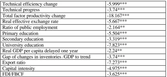
The stationnarity test of Im-Pesaran-Shin allows us to reject the unit root hypothesis for all variables in our estimation (see table 2). The results of Breusch and Pagan LM test and Hausman specific test indicate that we cannot reject the hypothesis of one model with fixed effects (see table 2).

The main potential econometric problem concerns the endogeneity of independent variables. We remind in introduction the Balassa-Samuelson effect that supposes an inverse relation to that tested here between productivity growth and real exchange rate. The endogeneity problem is also possible for the other independent variables which are of a macro-economic nature. We have shown (Guillaumont Jeanneney and Hua, 2002) that by applying the Balassa-Samuelson effect, the real effective exchange rate of Chinese provinces is explained by the ratio of the GDP of each province to that of its foreign trading partners17 on the one hand and to the GDP of China as a whole on the other hand. These variables are used here as instruments of exchange rate. For export rate, ratio of foreign direct investments, capital intensity and ratio of changes in inventories, the instruments are constituted by the variables themselves with a lag of one year and by a dummy variable equal to one for coastal provinces. The results of DWH test do not allow us to reject the endogeneity of these variables (see table 3). The results of Pagan/hall heteroskedasticiy test, which is the most pertinent in estimation with instrumental variables, allow us to prefer a Generalized Moments Model with instrumental variables to a model with fixed effects (Baum, Schaffer and Stillman, 2003). Finally, the pertinence and the validity of the instruments are tested using the Sargan over-identification test. The results do not allow us to reject the hypothesis that the instruments are independent of error terms.

16

The choice of custom data is justified particularly since 2000, Ministry refers to the same data. 17

4.3. Results of econometric estimations

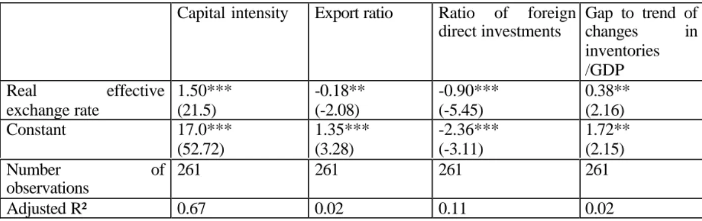
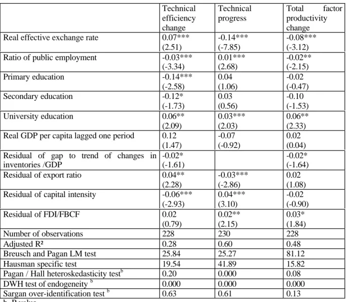
Econometric results are reported in tables 3 to 5. Table 3 presents the regression results of the basic model that includes all intermediate variables corresponding to transmission channels of the real exchange rate to productivity. Thus the coefficients relative to the real exchange rate represent its direct impact on productivity growth, which does not result of its action on the intermediate variables. Table 4 presents the regressions of intermediate variables on the real exchange rate. The results show that they actually are transmission channels of the real exchange rate to productivity growth. The residuals of these regressions are then substituted to intermediate variables for productivity growth estimations. The results of these new estimations presented in table 5 show the total impact of the real exchange rate on productivity growth and on its two components.

According to the results reported in these tables, most coefficients are significant with the expected signs.

We can see from tables 3 and 5 that the greater the proportion of the population which attains university education level is, the faster the efficiency change and the technical progress are obtained, while the impact of the other two education levels is negative or not significant. As expected, the more the public enterprises are important, the more the technical progress is strong and the efficiency improvement weaker.

The results relative to intermediate variables or transmission channels of the real exchange rate to productivity are also meaningful. The export ratio exerts a positive effect on efficiency, but a negative one on technical progress. The foreign direct investments favour technical progress as capital intensity does, while capital intensity is a factor of less efficiency improvement. Finally, the diminution of total demand related to the business cycle (measured by changes in inventories) lessens technical efficiency by reducing the utilization ratio of production capacities.

Table 3 allows us to measure the residual impact of the real exchange rate on productivity, which means the impact that does not result of the variations of the intermediate variables; while table 5 allows us to estimate the total effects of the real exchange rate. We observe that, according to table 3, the real effective exchange rate exerts a positive impact on technical efficiency and thus

a real appreciation does increase efficiency, probably due to higher competition pressure. On the contrary the real exchange rate exerts a negative impact on technical progress, and thus a real appreciation hinders technical progress probably by decreasing industrial sector progression. Finally the direct impact of the real exchange rate on total factor productivity is not significantly different from zero.

The total impact of the real exchange rate on productivity growth depends obviously on the impact of the real exchange rate on the intermediate variables identified as channels of transmission. Table 4 indicates that a real appreciation, as expected, exerts a negative effect on exports and foreign direct investments by decreasing competitiveness of provinces; and it has a positive effect on capital intensity due to the relative price decrease of imported equipment goods (cf. table 1). Moreover a real appreciation exerts an unfavorable short run effect on economic activity which is captured by the positive sign of the variable concerning changes in inventories.

By comparing tables 3 and 5, we observe that if the total impact of the real exchange rate remains significant, positive for efficiency and negative for technical progress, this total impact is significantly less important than the only direct impact, since the coefficients pass respectively from +0.18 and -0.18 for efficiency and technical progress (in table 3) to +0.07 and -0.14 (in table 5). The result is that the total impact of the real exchange rate on total factor productivity is significantly negative (-0.08).18 In other words, the real appreciation of exchange rate in the nineties have contributed to improve technical efficiency, to diminish the technical progress, and finally to reduce total factor productivity.

18

As real effective exchange rate has negative effect on exports and foreign direct investments, and these variables exercise the first one a positive effect on efficiency and the second one technical progress, the introduction of the residuals of functions in table 4 should decrease the coefficient relative to real effective exchange rate (should lead it less positive for efficiency but more negative for technical progress). The real appreciation exercises inversely positive effect on capital intensity. The introduction of residuals increases the coefficients of real effective exchange rate (more positive for efficiency, but less negative for technical progress). These effects offset each other partially to give the results in table 5.

5. Conclusion

Three main lessons emerge from our analysis.

The development of university education is actually one priority objective of the Chinese government. This strategy is completely justified by the positive impact of this education level on productivity growth, in particular on efficiency.

On the other hand, Japan and the United–States exert strong pressures on China government in order that it re-values the Renminbi. As regards the possible impact of a new appreciation of the Renminbi on the productivity in China, what is implied by our analysis is ambiguous. In the past it seems that the real appreciation has contributed to slow down productivity growth by curbing the path of technical progress. But this negative impact on technical progress has been dampened because the real appreciation has increased the capital-labour ratio and reduced the growth of exports. Moreover it has been partially compensated by a positive impact of the appreciation on efficiency. However, in the future, it is likely that export growth lead to more innovations, as China will increase higher technology exports (for instance electronic products). Actually the negative impact of the real appreciation on productivity growth has been small. Knowing that the annual average growth of the real effective exchange rate has ranged from 2.6% to 6.6% in the different provinces, the productivity growth has been reduced from 0.2 to 0.5 points of percentage for an average annual growth of productivity equal to 2.2%. However the striking fact is that according to the Malmquist index the efficiency has fallen in China from 1993 to 2001 at a rate of 0.3% a year. So the true stake of the transition of China towards a market economy is the efficiency improvement. We have shown that the real appreciation is a factor of better efficiency.

Finally, the significant relationships between real exchange rate on the one hand, exports, foreign direct investments, capital-labour ratio, business cycle and productivity growth on the other hand, clearly show that during the last decade China has become a market economy where economic agents adjust their behaviour to price signals.

References

Aigner, D.J., Lovell C.A.K. and Schmidt P.J., 1977, Formulation and estimation of stochastic frontier models, Journal of Econometrics, 6 (2), 21--37.

Baum C.F., Schaffer M.E. and Stillman S., 2003, Instrumental Variables and GMM Estimation and Testing, Working Paper No. 545, February, Department of Economics, Boston College.

Balassa B., 1964, The Purchasing Power Parity Doctrine: a Reappraisal,” Journal of Political Economy, 72, 584--596.

Balassa B.,1994, La théorie de la parité du pouvoir d’achat, un réexamen, Revue d’Economie du Développement, 2 (1), 17--34.

Caves, D.W. Christensen L.R. and Diewert W.E., 1982, Multilateral comparisons of output, input and productivity using superlative index numbers, Economic Journal, 92, 73--86.

Chen Y. and S. Démurger, 2002, La croissance de la productivité dans l’industrie manufacturière chinoise, le rôle de l’investissement direct étranger, Economie internationale, 92(4), 131--164.

Cortèse L. and P. Hua, forthcoming, The Effect of the Real Exchange Rate on Technological Progress



An Application to the Textile Industry in China, Current Politics and Economics of Asia.

Courchene T and R. Harris, 1999, Canada and North American Monetary Union, Canadian Business Economics, 7 (4), 5--14.

Dayal-Gulati A. and A.M. Husain, 2002, Centripetal Forces in China’s Economic Takeoff, IMF Staff Papers, 49(3), 364--393.

Dées S., 2002, Compétitivité-prix et hétérogénéité des échanges extérieurs chinois, Economie internationale, 92 (4), 41--66.

Démurger S., 1999, Infrastructures, éducation et croissance régionale en Chine , Revue d'Economie du Développement, n° spécial "Economie chinoise" : croissance et disparités, 1-2, 71--93.

Färe R., Grssskopf S., Norris M., and Z. Zhang, 1994, Productivity Growth, Technical progress, and Efficiency Change in Industrialized Countries, American Economic Review, 84 (1), 66--83.

Farrell, M. J., 1957, The measurement of productive efficiency, Journal of the Royal Statistical Society, series A, general 120, 253-82.

Feder G., 1983, On Exports and Economic Growth, Journal of Development Economics, 12, 1-2, 59--73.

Grubel H.G., 1999, The Case for the Amero: The Merit of Creating a North American Monetary Union, Fraser Institute, Vancouver, Canada.

Guillaumont P., 1994, Politique d’ouverture et croissance économique: les effets de la croissance et de l’instabilité des exportations, Revue d’économie du développement, 1, 91--114. Guillaumont S. and P. Hua, 2001, How does real exchange rate influence income inequality

between urban and rural areas in China? Journal of Development Economy, 64, 529--545. Guillaumont S. and P. Hua, 2002, The Balassa–Samuelson effect and inflation in the Chinese

provinces, China Economic Review, 108, 1–27.

Harris R.G., 2001, Is there a Case for Exchange Rate Induced Productivity Changes, mimeo Department of Economics, Simon Fraser University, Canadian Institute for Advanced Research.

Kalirajan K.P., Obwona M.B. and S. Zhao, 1996, A decomposition of total factor productivity growth: the case of Chinese agricultural growth before and after reforms, American Journal of Agricultural Economics, 78, 331--38.

Krugman P., 1989, Surévaluation et accélération des productivités : un modèle spéculatif, in Laussel D. and C. Montet (Eds.), Commerce international et concurrence parfaite, Paris, Economica, 121--135.

Leibenstein H., 1957, Economic Backwardness and Economic Growth, New-York, Wiley.

Leibenstein H., 1966, Allocative Efficiency versus X-Efficiency, American Economic Review, June, 392--415.

Lemoine F., 2002, La Chine dans l’économie mondiale : présentation, Economie internationale, 92, 4, 5--10.

Lin Y.F. and B.L. Liu, 2002, The strategy of development of Chinese economy and the regional income disparity, CCER, working paper, (in Chinese), no. 2002015.

Lu D. and Y. Qiao, 1999, Hong Kong’s Exchange Rate Regime: Lessons from Singapore, China Economic Review, 10, 122-140.

Mzzusen W. and J. Van des Broeck, 1977, Efficiency estimation from Cobb-Douglas production functions with composed error, International Economic Review, 18 (2), 435--44.

Naughton, B., 1999, How much can regional integration do to unify China’s Markets? Paper for the Conference on Policy Reform in China, Center for Research on Economic Development and Policy Research, Working Paper, Stanford University, 18-20, November.

Nishimizu M. and J.M. Page, 1982, Total factor productivity growth, technological progress and technical efficiency change: dimensions of productivity change in Yugoslavia, 1965-78, Economic Journal, 92, 920--36.

Porter M.E., 1990, The Competitive advantage of Nations, Cambridge, Mass, Harvard University Press.

Samuelson P., 1964, Theoretical Notes on Trade Problems, Review of Economics and Statistics, 46, 145--154.

Wu Y., 1999, Productivity and Efficiency in China's Regional Economics, in Tsu-Tan Fu et al., Economic Efficiency and Productivity Growth in the Asian-Pacific Region, Edward Elgar. Yue C.J. and Hua P., 2002, Does comparative advantage explains export patterns in China? China

Table 1: Expected impacts of the real exchange rate (an increase corresponds to an appreciation) on efficiency change, technical progress and productivity change

Impact of exchange rate on intermediate variables

Impact of intermediate variables on productivity growth

Impact of exchange rate on productivity growth

→

+ _{Technical efficiency}

→

− _{Technical efficiency}

→

?

Technical progress

→

? Technical progress

→

− _{Openness to outside}

→

?

Total productivity

→

? Total productivity

→

+ _{Technical efficiency}

→

− _{Technical efficiency}

→

+ _{Technical progress}

→

− _{Technical progress}

→

− _{Foreign direct}

investments

→

+ _{Total productivity}

→

− _{Total productivity}

→

− _{Technical efficiency}

→

− _{Technical efficiency}

→

+ _{Technical progress}

_→

+ _{Technical progress}

Indirect impact of exchange rate

→

+ _{Capital intensity}

→

?

Total productivity

→

? Total productivity

→

+ _{Technical efficiency}

→

− _{Technical progress}

Direct impact of exchange rate

→

? Total productivity

→

? Technical efficiency

→

? Technical progress Total impact of exchange rate

→

?

Table 2. Stationnarity test of Im-Pesaran-Shina

Technical efficiency change -5.999***

Technical progress -3.74***

Total factor productivity change -18.167***

Real effective exchange rate -5.667***

Ratio of public employment -2.164**

Primary education -5.504***

Secondary education -3.319***

University education -7.823***

Real GDP per capita delayed one year -2.24** Gap of changes in inventories /GDP to trend -3.74***

Export ratio -7.273***

Capital intensity -4.975***

FDI/FBCF -3.625***

Table 3. Estimation of productivity growth and its components: basic model Technical efficiency change Technical progress Total factor productivity

Real effective exchange rate 0.18***

(4.30)

-0.18*** (-8.68)

-0.02 (-0.54)

Ratio of public employment -0.03***

(-3.34) 0.01*** (2.68) -0.02** (-2.15) Primary education -0.14*** (-2.58) 0.04 (1.06) -0.02 (-0.47) Secondary education -0.12* (-1.73) 0.03 (0.56) -0.10 (-1.53) University education 0.06** (2.09) 0.03*** (2.03) 0.06** (2.33) Real GDP per capita lagged one period 0.12

(1.47)

-0.07 (-0.92)

0.02 (0.04) Gap to trend of changes in inventories/GDP -0.02*

(-1.61) -0.02* (-1.64) Export ratio 0.04** (2.28) -0.03*** (-2.86) 0.02 (1.08) Capital intensity -0.06*** (-2.93) 0.04*** (3.10) -0.02 (-0.90) FDI/FBCF 0.02 (0.79) 0.02** (2.15) 0.03* (1.84) Number of observations 228 2280 228 Adjusted R² 0.28 0.60 0.48

Breusch and Pagan LM test 25.84 25.27 81.12

Hausman specific test 19.54 41.89 15.82

Pagan / Hall heteroskedasticity testb 0.20 0.000 0.08

DWH test of endogeneity b 0.000 0.000 0.000

Sargan over-identification test b 0.63 0.61 0.13

Table 4: Estimation of transmission channels of the real exchange rate to productivity Capital intensity Export ratio Ratio of foreign

direct investments Gap to trend of changes in inventories /GDP Real effective exchange rate 1.50*** (21.5) -0.18** (-2.08) -0.90*** (-5.45) 0.38** (2.16) Constant 17.0*** (52.72) 1.35*** (3.28) -2.36*** (-3.11) 1.72** (2.15) Number of observations 261 261 261 261 Adjusted R² 0.67 0.02 0.11 0.02

Table 5. Estimation of total impact (direct and indirect) of the real exchange rate on productivity change and on its components Technical efficiency change Technical progress Total factor productivity change

Real effective exchange rate 0.07***

(2.51)

-0.14*** (-7.85)

-0.08*** (-3.12)

Ratio of public employment -0.03***

(-3.34) 0.01*** (2.68) -0.02** (-2.15) Primary education -0.14*** (-2.58) 0.04 (1.06) -0.02 (-0.47) Secondary education -0.12* (-1.73) 0.03 (0.56) -0.10 (-1.53) University education 0.06** (2.09) 0.03*** (2.03) 0.06** (2.33) Real GDP per capita lagged one period 0.12

(1.47)

-0.07 (-0.92)

0.02 (0.04) Residual of gap to trend of changes in

inventories /GDP

-0.02* (-1.61)

-0.02* (-1.64)

Residual of export ratio 0.04**

(2.28)

-0.03*** (-2.86)

0.02 (1.08)

Residual of capital intensity -0.06***

(-2.93) 0.04*** (3.10) -0.02 (-0.90) Residual of FDI/FBCF 0.02 (0.79) 0.02** (2.15) 0.03* (1.84) Number of observations 228 230 228 Adjusted R² 0.28 0.60 0.48

Breusch and Pagan LM test 25.84 25.27 81.12

Hausman specific test 19.54 41.89 15.82

Pagan / Hall heteroskedasticity testb 0.20 0.000 0.08

DWH test of endogeneity b 0.000 0.000 0.000

Sargan over-identification test b 0.63 0.61 0.13

Table A1. Evolution of total factor productivity and its two components in three Chinese regions

Eastern Center Western

Technical Efficiency Technical progress Total Productivity Technical Efficiency Technical progress Total Productivity Technical Efficiency Technical progress Total Productivity 1993 0,99 1,07 1,06 0,98 1,07 1,04 0,97 1,07 1,04 1994 0,98 1,06 1,04 1,00 1,04 1,04 0,98 1,05 1,03 1995 1,00 1,03 1,03 1,02 1,00 1,02 1,01 1,01 1,02 1996 0,99 1,03 1,02 1,02 1,02 1,04 1,01 1,02 1,03 1997 0,99 1,03 1,03 1,01 1,01 1,02 1,00 1,01 1,01 1998 1,00 1,02 1,02 1,01 0,99 1,00 1,01 1,00 1,00 1999 1,00 1,05 1,04 0,99 1,01 1,00 0,98 1,01 0,99 2000 1,00 1,03 1,02 1,00 1,00 1,00 0,99 1,01 1,00 2001 1,00 1,02 1,02 1,00 1,01 1,01 0,99 1,01 1,00 Average 1,00 1,04 1,03 1,00 1,02 1,02 0,99 1,02 1,01

Table A2. Geometric average of total factor productivity of Chinese provinces and its two component from 1993 to 2001

Technical efficiency Technical progress Total factor productivity

BEIJING 0,986 1,032 1,017 TIANJIN 1,009 1,039 1,048 HEBEI 0,983 1,015 0,998 SHANXI 0,975 1,014 0,988 INNER MONGOLIA 0,991 1,014 1,005 LIAONING 1,009 1,049 1,059 JILIN 1,012 1,017 1,029 HEILONGJIANG 1,002 1,037 1,038 SHANGHAI 1 1,081 1,081 JIANGSU 1,004 1,042 1,046 ZHEJIANG 0,984 1,038 1,022 ANHUI 1,028 1,015 1,044 FUJIAN 1,005 1,024 1,03 JIANGXI 1,001 1,004 1,005 SHANDONG 1,01 1,017 1,027 HENAN 1,002 1,015 1,017 HUBEI 0,998 1,015 1,014 HUNAN 1,013 1,015 1,028 GUANGDONG 1 1,041 1,041 GUANGXI 0,975 1,007 0,982 SICHUAN 0,995 1,016 1,011 GUIZHOU 0,99 1,011 1,001 YUNNAN 0,984 1,015 0,998 SHAANXI 1,002 1,015 1,017 GANSU 1,017 1 1,017 QINGHAI 0,988 1,018 1,006 NINGXIA 0,997 1,034 1,03 XINJIANG 0,976 1,046 1,021 HAINAN 0,979 1,049 1,027 Average 0,997 1,025 1,022

Figure 1

Real Effective Exchange Rate of China (1995=100)

Figure 2

Annual average rate of appreciation of the real effective exchange rate from 1993 to 2001

Figure 3

Decomposition of output growth rate

Figure 4

Malmquist indices relative to total factor productivity and its two components (geometric

average of Chinese provinces)