SOFT feature tracking software handbook

(1)

SOFT

Satellite-Based Ocean Forecasting

EVK3-CT-2000-00028

Coordinator: Dr. Joaquín Tintoré

Feature-Tracking Software Handbook

WP 3 – Task 3.1

Development of feature tracking methods

Distribution 2.0 - September 2003

Paolo Cipollini, Peter Challenor

Southampton Oceanography Centre, U.K.

(2)

2

Contents

I

NTRODUCTION

... 3

D

ATA USED

... 4

S

OFTWARE DESCRIPTION

... 5

T

ABLE OF ROUTINES

... 9

R

EFERENCES

... 10

APPENDIX – P

ROGRAM LISTINGS

... 11

gapfill_gaussian_2d.m ... 11

gauss_wave_tap.m... 13

gauss2d.m ... 14

soft_compact.m... 15

soft_ltpfit.m ... 16

soft_main.m ... 20

soft_nofwaves.m ... 23

soft_output_results.m ... 24

soft_paramsmaps.m... 25

soft_reconstruct.m ... 26

soft_rerun_wavejoin.m... 28

soft_singlefit.m ... 29

soft_wavecrop.m... 31

soft_wavefind.m... 32

soft_wavescreen.m... 36

soft_wavetrackplotter.m... 37

(3)

Introduction

This handbook (

SOFT_WP31_handbook.pdf

) describes the suite of MATLAB

programs developed within Work Package 3, task 3.1 of the SOFT Project, for the

tracking of large-scale, westward propagating features

(planetary waves or

westward-travelling eddies) in altimeter data and the removal of the identified features

from the

datasets

. The suite has been applied to TOPEX/POSEIDON data over the

Azores region (one of the SOFT study regions) but its modularity makes it adaptable in

a straightforward way to other datasets and other regions.

The companion to this handbook is the progress report on task 3.1 released in

January 2003 (

SOFT_WP31_report.pdf

), which presents the rationale to the study and

gives ample details on the scheme adopted for the fitting of elementary waves

(according to a Gaussian wave shape model) to altimeter data. A synopsis of the fitting

scheme is briefly recalled in the following sections of this document, for the benefit of

the reader. All the code listings are in the appendix.

The forecasting of the westward-propagating fields (which is the object of task

3.2 in Work Package 3 id described in version 1 of another report,

SOFT_WP32_rep1.pdf

)

All documents and data relevant to Work Package 3 of the SOFT Project,

including all the code and data described in this handbook, can be downloaded via

anonymous FTP from

f t p . s o c . s o t o n . a c . u k

under directory

/ p u b / s o f t /

distribution2

. That directory is further subdivided into:

-

…/data

: fitting results plus some ancillary data

-

…/fitting

: fitting routines

-

…/forecast

: forecast code (for task 3.2 – see

SOFT_WP32_rep1.pdf

)

-

…/utils

: various utilities for data management, screening and plotting

(4)

4

Data used

For the preparation of the wave-fitting software (detailed in the previous report

SOFT_WP31_report.pdf

) and the first release (distribution 1.0) of the

results we had

used TOPEX/Poseidon SSH anomalies calculated with respect to the 1993-1995 mean

at each location along the satellite ground track, and gridded on a 1° x 1° x 1 orbital

cycle grid (1 orbital cycle=9.9156 days). These data are part of the GADGET archive of

gridded satellite data at the Southampton Oceanography Centre (SOC), and are

available both in MATLAB and NetCDF format.

During early 2003 we obtained from CLS Space Oceanography Division in

Toulouse their MSLA product, a merged TOPEX/Poseidon + ERS altimetric product,

consisting of optimally-interpolated SSH anomalies on a 0.25° x 0.25° x 10 day grid,

and produced in the framework of the Environment and Climate EU AGORA

(ENV4-CT9560113) and DUACS (ENV44-T96-0357) Projects. The details of the optimal

interpolation are covered in Le Traon and Dibarboure (1999), Ducet et al. (2000) and Le

Traon et al. (2001). The CLS MSLA product reproduces the large-scale and meso-scale

ocean variability better than the GADGET product, so in this phase of the project we

have decided to adopt the CLS dataset and at the same time we have streamlined and

modified several of the SOFT fitting routines described in this handbook so that they

can be straightforwardly run on data gridded on any grid.

The current distribution (distribution 2.0) of the SOFT WP 3.1 data is therefore

based on the merged T/P+ERS CLS MSLA. In the analysis described below we covered

the region 20°N to 40°N and 75°W to 8°W, which we refer to in the following as ‘the

study area’, and used 232 10-day cycles of CLS MSLA covering from early April 1995

to early August 2001.

(5)

Software description

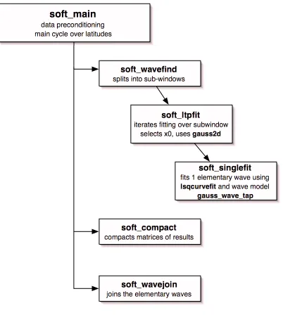
A scheme of the MATLAB routines used in the fitting is in figure 1. The

relevant files are in the FTP archive under

/pub/soft/distribution2/fitting

and

/pub/soft/distribution2/utils

(the program listings are in the appendix). In the

figure and in the following text, routine names are in

bold

(all MATLAB routines have

extension

.m

, which is omitted in the following).

The approach followed to identify the single waves at any given latitude,

described in detail in the earlier report

SOFT_WP31_report.pdf

and in Cipollini

(2003), can be summarized as follows:

a)

split the full longitude/time plot into a number of overlapping sub-windows

b)

for each sub-window, fit a number of

elementary waves

by minimizing the

mean square error with respect to a wave shape model

c)

reconstruct the trajectories of any single wave event by ‘joining’ the

elementary waves in a sub-window with those in the adjacent window to the

west

The main program for wave fitting is

soft_main

. This cycles over the latitudes

and at any latitude extracts the longitude/time section of the data (covering the entire

longitude section, except for any land on the sides). Then it performs some

preconditioning of the longitude/time plot: it fills any gaps with

gapfill_gaussian_2d

and then zero-pads the plot, filters it with

westward_filter

and re-crops it to the original

size. The particular filter adopted is a westward-only filter, that is a filter that in the

wavenumber/frequency space (the 2-D Fourier Transform of the longitude/time space)

removes the quadrants containing the eastward propagation, plus the two axis

wavenumber=0 and frequency=0 (thus removing any stationary signal). To improve the

removal of the annual component, it also removes a 3 x 3 cluster of spectral bins around

the zero-wavenumber, annual peak in the wavenumber/frequency space. Subsequently,

(6)

6

soft_main

data preconditioning

main cycle over latitudes

soft_waveﬁnd

splits into sub-windows

soft_ltpﬁt

iterates ﬁtting over subwindow

selects x0, uses

gauss2d

soft_singleﬁt

ﬁts 1 elementary wave using

lsqcurveﬁt

and wave model

gauss_wave_tap

soft_compact

compacts matrices of results

soft_wavejoin

[image:6.595.103.505.73.521.2]

joins the elementary waves

Figure 1 - Scheme of the MATLAB routines used in the fitting.

The core of the fitting routines is formed by

soft_ltpfit

and

soft_singlefit

. The

first one,

soft_ltpfit

, is called by

soft_wavefind

and fits a number of elementary shapes

(waves) to a sub-window, in an iterative way, and calling in turn

soft_singlefit

to do the

fitting of each single wave. The fitting is done with a Levenberg-Marquardt

least-squares optimization (function

lsqcurvefit

in the MATLAB Optimization Toolbox)

with respect to a wave shape model. The model adopted is a tapered Gaussian model (in

gauss_wave_tap

) where each feature is identified by 4 parameters

(

A

,

s

,

p

,

σ

), that is its

amplitude, slope, intercept and width, respectively (see the previous report

(7)

image). If for a particular quadruplet (

A

₀

,

s

₀

,

p

₀

,

σ

₀

)

soft_singlefit

does not converge, the

relevant feature in the longitude/time plot is masked out with a gaussian mask (using

gauss2d

), so that the peak in the Radon Transform disappears and the code moves to

testing other peaks (other features).

In distribution 1.0 of the data, we provided to the other Project partners the

residuals’ field, simply compacted with

soft_compact,

for use into other work packages

(like Work Package 2 for the testing of the non-linear time series predictors). From

distribution 2.0, we also provide the partners with a field of ‘selected residuals’ which is

better suited to represent the non-fitted (residual) variability and thus should be used

instead of the old one. These selected residuals have been created as follows: first we

select (using utility

soft_wavescreen

) only those waves that propagate for at least 3°

longitude in the dataset (this excludes any very localized feature that may have been

fitted by the fitting code), then we use those waves to create a reconstructed wave field

with the utility

soft_reconstruct

, and finally we computed the selected residuals as the

difference between the original (unfiltered) longitude/time plots and the reconstructed

wavefield. As we only use selected waves (with

soft_wavescreen

) for the wave

forecast, the selected residuals field contains all the remaining variability and can be

used by the partners for their predictions. Their forecasts is going to be merged with the

forecasted propagation of the single wave events (which are identified as explained

below) from Work Package 3.2 – this constitutes the hybrid SOFT tracking method.

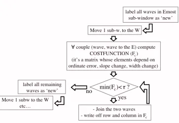
For the sake of clarity we recall here the strategy of the wave joining program

soft_wavejoin

, as schematized in figure 2. We start from the easternmost sub-window

and its associated table of elementary waves, each one identified by a set of four

parameters (

A

,

s

,

p

,

σ

). We label each one of these easternmost waves as ‘new’ and then

we move to the next sub-window to the west. We compare each elementary wave in this

sub-window with each elementary wave in the previous one by evaluating a

cost

function

of the wave pair, depending on the mismatch between their slopes, intercepts

and widths (a further dependence on amplitude mismatch can be added if wanted). In

the

cost function matrix

F

c

so obtained (where any row corresponds to an elementary

wave in the new sub-window and any column to an elementary wave in the previous

sub-window) we find the minimum cost, and if it is below an acceptance threshold we

‘join’ the two waves, that is we classify the elementary wave in the new sub-window as

a continuation of the one to the east, and write off the relevant row and column in the

matrix so that the two waves cannot be joined to any others. Once all the minima below

the cost threshold in F

_c

have been accounted for, we label all the remaining waves as

‘new’ and move to the next sub-window to the west, and so on. The result is in the form

of a MATLAB data structure, that is a structured table where any entry represents a

‘joined’ wave (that is, a single wave event made by one or more elementary waves), and

lists the evolution of its parameters with longitude.

(8)

[image:8.595.111.474.104.354.2]

8

(9)

[image:9.595.86.518.157.632.2]

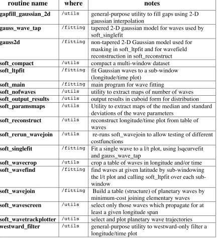
Table of routines

For a detailed help on each routine, see help lines in the program listings in the

Appendix, or type ‘help routinename’ at the MATLAB command prompt

routine name

where

notes

gapfill_gaussian_2d

/utils

general-purpose utility to fill gaps using 2-D

gaussian interpolation

gauss_wave_tap

/fitting

tapered 2-D gaussian model for waves used by

soft_singlefit

gauss2d

/fitting

non-tapered 2-D Gaussian model used for

masking in soft_ltpfit and for wavefield

reconstruction in soft_reconstruct

soft_compact

/utils

compact a multi-window dataset

soft_ltpfit

/fitting

fit Gaussian waves to a sub-window

(longitude/time plot)

soft_main

/fitting

main program for wave fitting

soft_nofwaves

/utils

utility to extract maps of number of waves

soft_output_results

/utils

output results in cuboid form for distribution

soft_paramsmaps

/utils

Utility to extract maps of the median and standard

deviations of the wave parameters

soft_reconstruct

/utils

reconstruct longitude/time plot from table of

waves

soft_rerun_wavejoin

/utils

re-runs soft_wavejoin to allow testing of different

costfunctions

soft_singlefit

/fitting

Fit a single wave to a l/t plot, using lsqcurvefit

and gauss_wave_tap

soft_wavecrop

/utils

crop a table of waves in longitude and/or time

soft_wavefind

/fitting

find waves at given latitude by sub-windowing

the l/t plot and calling soft_ltpfit over each

sub-window

soft_wavejoin

/fitting

Build a table (structure) of planetary waves by

minimum-cost joining elementary waves

soft_wavescreen

/utils

select only those waves which propagate for at

least a given longitude span

soft_wavetrackplotter

/utils

select and plot planetary wave trajectories

westward_filter

/utils

general-purpose utility to westward-only filter a

(10)

10

References

Cipollini, P., 2003: Multiple satellite observations of oceanic planetary waves:

techniques and findings.

Proceedings of 2003 Tyrrhenian International Workshop on

Remote Sensing

, ed. by E. Dalle Mese, pp 134-143, Edizioni Plus, Uni. of Pisa, Italy.

ISBN 88-8492-291-7

Ducet, N., P.-Y. Le Traon, and G. Reverdin, 2000: Global high resolution mapping of

ocean circulation from TOPEX/Poseidon and ERS-1 and -2.

J. Geophys. Res.

,

105,

19477-19498.

Le Traon, P.-Y. and G. Dibarboure, 1999: Mesoscale mapping capabilities of

multi-satellite altimeter missions.

J. Atmos. Oceanic Technol.

,

16,

1208-1223.

(11)

APPENDIX – Program listings

gapfill_gaussian_2d.m

function filled=gapfill_gaussian_2d(S,mask,fwhm_x,sr_x,fwhm_y,sr_y,vflag) % GAPFILL_GAUSSIAN_2D fills gaps using 2-D gaussian interpolation

% FILLED=GAPFILL_GAUSSIAN_2D(S,MASK,FWHM_X,SR_X,FWHM_Y,SR_Y) fills % the gaps in matrix S (only in those locations where the 2-D MASK is % 1) using a gaussian interpolation scheme whose full-width half-maxima % and search radii in x and y and z are FWHM_X,SR_X,FWHM_Y,SR_Y

% (all expressed in pixel units). %

% FILLED=GAPFILL_GAUSSIAN_2D(...,'verbose') displays the number of gaps % to be filled during execution

%

% See also GAPFILL_GAUSSIAN_3D, MAPGAPFILL and, in the Image Processing % Toolbox, IMFILL and BWFILL.

% V 1.1 Paolo Cipollini 04/09/2003

% Version History

% V 1.1 Paolo Cipollini 04/09/2003 Added vflag

% V 1.0 Paolo Cipollini 28/09/1999 saved 15/01/2002 with comments

switch nargin case 6

vflag='n'; case 7

otherwise

disp('Wrong number of arguments'); filled=[]; return end

warning off

filled=S;

[nr,nc]=size(S);

sr_x=floor(sr_x); % x search interval in pixels sr_y=floor(sr_y); % y search interval in pixels

sigmax=0.8493*fwhm_x; sigmay=0.8493*fwhm_y;

% Computation of the 2-D gaussian weights x=-sr_x:sr_x; y=-sr_y:sr_y;

[X,Y]=meshgrid(x,y);

const=1/(sigmax*sigmay*(2*pi));

G=const*exp(-(X.^2)/(2*sigmax^2)-(Y.^2)/(2*sigmay^2));

% find where the gaps to fill are

[idr,idc]=find(isnan(S) & mask); %idc=rem(idct-1,nc)+1;

%idt=floor((idct-1)/nc)+1;

gapno=length(idr);

if strcmp(lower(vflag),'verbose')==1,

disp(['Number of gaps: ' num2str(gapno)]) end

fillerflag=0;

% For each gap ----for i=1:gapno,

r=idr(i);c=idc(i);

rspan=r-sr_y:r+sr_y; rspan(find(rspan<1))=1; rspan(find(rspan>nr))=nr; cspan=c-sr_x:c+sr_x; cspan(find(cspan<1))=1; cspan(find(cspan>nc))=nc;

buf=S(rspan,cspan);

(12)

12

filled(r,c)=nansum(W(:))/sum(G(idx));

if strcmp(lower(vflag),'verbose')==1,

if mod(i,1000)==0,disp(['Done ' num2str(i) ' of ' num2str(gapno)]),end; end

end

if strcmp(lower(vflag),'verbose')==1, disp(['Filling completed']) end

warning backtrace

(13)

gauss_wave_tap.m

function G=gauss_wave_tap(x,xdata)

% GAUSS_WAVE_TAP tapered 2-D gaussian model for waves %

% Function used by soft_solifit in the SOFT wave tracking % Usage:G=gauss_soliton_tap(x,xdata)

% where: x=[x1 x2 x3 x4], parameters vector % x1=amplitude

% x2=slope

% x3=y-intercept

% x4=width (std_x of gaussian) % xdata:matrix of x and y values (domain)

% (due to the way optimization routines work, the matrices % with the values of x and y, obtained with meshgrid from % the vectors defining the grid, need to be rearranged % into a single matrix, as in the following example:

% [xmat,ymat] = meshgrid(lon-lon_central,time);

% xdata=[xmat ymat];

%

% GAUSS2D is a simpler form of the same function (but it is not suited to % be used in the optimization process and IT IS NOT TAPERED)

%

% This code is part of a suite of programs developed at the % Southampton Oceanography Centre, U.K., within the framework % of the Energy, Environment and Sustainable Development EU % Project SOFT (Satellite-based Ocean ForecasTing) - contract % number EVK3-CT-2000-00028

%

% Codes and documentation are available via anonymous FTP from % ftp.soc.soton.ac.uk under /pub/soft

%

% V 2.0 05 July 2003 Paolo Cipollini (rev. 09/03)

% Version history

% V 2.0 05 July 2003 Paolo Cipollini:

% - renamed GAUSS_WAVE_TAP as old name % GAUSS_SOLITON_TAP was inappropriate % - uses y-intercept rather than x-intercept % - uses REPMAT to create the tapering matrix %

% V 1.0 17 January 2003 Paolo Cipollini - from GAUSS_SOLITON v 2.0 % originally developed by Stefano Colombo (sc3)

[nr,lx]=size(xdata); nc=lx/2;

tap=repmat(hanning(nc)',nr,1);

G = x(1)*exp(-((xdata(:,1:nc)-(xdata(:,(nc+1):lx)-x(3))./x(2)).^2)./(2*x(4)^2)); G = G.*tap;

(14)

14

gauss2d.m

function G2=gauss2d(vx,vy,x)

% GAUSS2D Simple 2-D Gaussian model for waves in a l/t plot % GAUSS2D(VX,VY,X) produces a Gaussian 'crest' or 'deep' % over the 2-D domain defined by vectors VX and VY. X is a % 4-element row vector with the parameters defining the % Gaussian surface, namely:

% X(1) = amplitude (positive->'crest' else 'trough') % X(2) = slope of the Gaussian trajectory

% x(3) = y-intercept of the Gaussian trajectory % x(4) = width (sigma of the Gaussian)

%

% GAUSS2D is in a form not suitable for fitting/optimization % purposes. Use GAUSS_WAVE (or its tapered version

% GAUSS_WAVE_TAP) instead %

%

% V 2.0 Paolo Cipollini July 2003 (rev. 09/03)

% VERSION HISTORY

% V 2.0 Paolo Cipollini July 2003 - uses y-intercept rather than % x-intercept

% V 1.0 Paolo Cipollini October 2002 - revised March 2003 % - uses x-intercept

[xmat,ymat]=meshgrid(vx,vy);

G2=x(1)*exp(-((xmat-(ymat-x(3))/x(2)).^2)./(2*x(4)^2));

(15)

soft_compact.m

function cpt=soft_compact(datacuboid,ls) % SOFT_COMPACT compact a multi-window dataset

% CPT = SOFT_COMPACT(DATACUBOID,LS) compacts a cuboid of long/time % plots (from a moving-window analysis with longitude step LS) into % a single plot, by taking the central part only of each plot and % joining them together. LS can be omitted in which case it is taken % to be 1

%

% V. 1.0 Paolo Cipollini 13/01/2003 (rev. 09/03)

% Version History

% V. 1.0 Paolo Cipollini 13/01/2003 -- from COMPACT with generalization

if nargin==1, ls=1; end

% take dimension of each window (nr,nc) and number of windows (nw) [nr nc nw]=size(datacuboid);

cpt=[];

for i=1:nw

if i==1 % westernmost subwindow

cpt=squeeze(datacuboid(:,1:(ceil(nc/2)-ceil(ls/2)+ls),i)); elseif i==nw % easternmost subwindow

cpt=[cpt, squeeze(datacuboid(:,(ceil(nc/2)-ceil(ls/2)+1):nc,i))]; else % intermediate subwindow

cpt=[cpt, squeeze(datacuboid(:,...

ceil(nc/2)-ceil(ls/2)+(1:ls),i))]; end

end

(16)

16

soft_ltpfit.m

function [elem_waves,stand_dev,residual]=soft_ltpfit(ltp,minslope,maxslope,plotflag)

% SOFT_LTPFIT Fit gaussian waves to a sub-window (l/t plot) %

% Use: [elem_waves,stand_dev,residual]=...

% soft_ltpfit(ltplot,minslope,maxslope,plotflag)

% Where: elem_waves = matrix of the fitted wave parameters % stand_dev = vector of residuals' standard_dev % residual= last residual of the iterations % minslope,maxslope = slope range

% (these also set the range of angle within which % to look for peaks in the RT)

% plotflag can be one of the following: % 'n' - no plotting

% 'plot' - displays plots during execution % 'print'- prints them as framexxx.eps %

%

% Version History

% V. 3.1 Paolo Cipollini 12/07/2003 different RT masking strategy, % and RT mask reset strategy

% 2nd time will only allow three failures

% fixed a small bug in residual computation on exit % V. 3.0 Paolo Cipollini 06/07/2003 -- major rehaul:

% introduced width0 % changed norm of RT

% changed a few variable names % used stdev instead of norm % repmat for tap

% minslope, maxslope rather than angles <---IMPORTANT % passes all bounds to optimizing routine

% normfactor not tapered

% V. 2.3 Paolo Cipollini 17/05/2003 -- plotflag can print/plot % V. 2.2 Paolo Cipollini 23/03/2003 -- added plotflag as input % and streamlined

% V. 2.1 Paolo Cipollini 22/01/2003 -- min,maxangle in input % V. 2.0 Paolo Cipollini 16/01/2003 -- new strategy: fitting % hanning-weighted gaussians

% V. 1.0 Paolo Cipollini 12/01/2003 -- From RESIDUAL_FIT % originally developed by Stefano Colombo

% * PREAMBLE ***

[nr nc]=size(ltp);

% nargin checks

if nargin==3, plotflag='n';end

% compute min, max angles from min, max slopes minangle=90+deg(atan(minslope));

maxangle=90+deg(atan(maxslope));

% preallocate matrices

elem_waves= []; %zeros(70,4)*nan; stand_dev= []; %zeros(70,1)*nan; %exit_flag= [];

failcount=0; % fail counter, counts number of failed attempts to fit a wave maxfails=10; % maximum number of failures before resetting or exiting maskresetcount=0; % counts the number of times the mask has been reset framecount=0; % frame counter, used for moviemaking purposes

width0=nc/10; % this could be computed or could be input arg

(17)

ltp_initial=ltp;

if strcmp(plotflag,'plot') | strcmp(plotflag,'print') figure

subplot(1,3,1);cipcolor(ltp_initial);shading flat;caxis([-.2 .2]);colorbar;pause(0.01);

end

disp(['Initial standard deviation of data = ' num2str(std(ltp_initial(:)))])

% create tapering matrix tap=repmat(hanning(nc)',nr,1);

% normalization factor for Radon Transform

normfactor=radon(ones(size(ltp)),1:89)+1; % normalization factor for RT

% definition of a mask for the Radon Transform

% this is multiplied for the data before doing the RT and it is % initially made of all ones - but

% when the program stalls over a particular maximum in the radon transform % a gaussian with the relevant slope and intercept is subtracted from the mask % so that the next RT*mask will have a different maximum and the stalling is % overcome. Note that the mask is always reset to all ones after finding % & removing a gaussian

mask=ones(size(ltp));

% tapering ltp=ltp.*tap;

ltp_tapered=ltp; % this will be the reference tapered data

% prepares second and third subplots

if strcmp(plotflag,'plot') | strcmp(plotflag,'print') subplot(1,3,2);

cipcolor(zeros(size(ltp)));shading flat;caxis([-.2 .2]);colorbar;pause(0.01); subplot(1,3,3);

cipcolor(ltp_tapered);shading flat;caxis([-.2 .2]);colorbar;pause(0.01); if strcmp(plotflag,'print')

print('-depsc2','-adobecset',...

['frame' num2str(100+framecount) ]);framecount=framecount+1; end

end

% start with 'residual' being the initial data (tapered) residual=ltp;

% MAIN FITTING CYCLE ****

while 1

stand=std(ltp(:));

if strcmp(plotflag,'plot') | strcmp(plotflag,'print')

disp(['Standard deviation of data at this stage = ' num2str(stand)]) end

% computes radon transform

RT=radon(flipud(ltp.*mask),1:89)./normfactor; [rowrt,colrt]=size(RT);

% restrict search to plausible angles

RTsubset=RT(:,floor(minangle):ceil(maxangle)); [pmax,thetamax]=find(abs(RT)==max(abs(RTsubset(:))));

% convert thetamax into slope slope=-tan(rad(90-thetamax));

% find y-intercept from RT -- here's how:

% first, find coordinates xc=0,yc of ltplot center

% consider the line through the center with angle thetamax:

% (that would be y=m*x+p where m=tan(rad(thetamax))=-1/slope and p=yc) % the maximum (or minimum) on that line is in pmax (in along-line coords), % and the midpoint of that line (corresponding to the center of the % ltplot) is in (rowrt+1)/2 so the maximum is offset by

% p1=pmax-(rowrt+1)/2 w.r.t. the center of the plot % the coordinates of the maximum on the ltplot are then % xm=xc+p1*cos(rad(thetamax)) ; ym=yc+p1*sin(rad(thetamax)) % and the normal to the line through that maximum is:

% y=(-1/m)*x+p with p=ym+(1/m)*xm

% whose y-intercept is p=ym+(1/m)*xm=ym+xm/m xc=0; yc=floor((nr+1)/2);

m=tan(rad(thetamax)); p1=pmax-(rowrt+1)/2;

(18)

18

intcep=ym+xm/m;

% fixes intcep between 0 and nr-1

intcep=max(0,intcep);intcep=min(intcep,nr-1);

if strcmp(plotflag,'plot') | strcmp(plotflag,'print')

%uncomment if you want trial line to disappear every time %subplot(1,3,3);

%cipcolor(residual);shading flat;caxis([-.2 .2]);colorbar;

% this is purely cosmetic: plot line under trial hold on plot([1,nc]+0.5,(([1,nc]+0.5)-floor((nc-1)/2)-1)*slope+(intcep+1)+0.5); hold off if strcmp(plotflag,'print') print('-depsc2','-adobecset',['frame' num2str(100+framecount) ]);framecount=framecount+1; end pause(0.01) end

% call single wave fitting routine if RT(pmax,thetamax)>0

x0=[0.1 slope intcep width0]; else

x0=[-0.1 slope intcep width0]; end

% prints x0

if strcmp(plotflag,'plot') | strcmp(plotflag,'print') x0,

end

%%%%%%%% call to soft_singlefit %%%%%%%%% [xout,resnorm,residual,exitflag]=...

soft_singlefit(x0,ltp,1000,0.01,1,minslope,maxslope,0-10,(nr-1)+10,width0/5,5*width0);

% prints xout and exitflag

if strcmp(plotflag,'plot') | strcmp(plotflag,'print') [xout exitflag]

%pause end

standnew=std(residual(:));

% wave acceptance checks

if (abs(xout(1))>1.2*stand & abs(xout(1))>0.02 &...

exitflag>0 & (stand-standnew)/stand>1/10000); % 1.2 selected empirically elem_waves(end+1,:)=xout;

stand_dev(end+1,:)=standnew; %exit_flag(end+1,:)=exitflag;

if strcmp(plotflag,'plot') | strcmp(plotflag,'print') elem_waves

subplot(1,3,2);

cipcolor(ltp_tapered-residual);shading flat;caxis([-.2 .2]);colorbar; subplot(1,3,3);

cipcolor(residual);shading flat;caxis([-.2 .2]);colorbar; if strcmp(plotflag,'print') print('-depsc2','-adobecset',['frame' num2str(100+framecount) ]);framecount=framecount+1; end pause(0.01) end ltp=residual;

failcount=0; % reset counter

else % add failed attempt (non-tapered) to RT mask

mask=mask-gauss2d((0:nc-1)-floor((nc-1)/2),0:nr-1,[1 slope intcep width0]); mask(find(mask<0))=0; % to prevent mask becoming negative

failcount=failcount+1; end

if failcount==maxfails,

(19)

if strcmp(plotflag,'plot') | strcmp(plotflag,'print') disp('--- mask reset -- '), beep; end

maskresetcount=maskresetcount+1;

failcount=0; maxfails=3; % 2nd time will only allow three failures else residual=ltp; break, end

end end

[gr gc]=size(elem_waves);

disp(['Fitted ' num2str(gr) ' Gaussians in this sub-window'])

(20)

20

soft_main.m

% SOFT_MAIN main program for SOFT wave tracking %

%

% V 3.1 Paolo Cipollini 12/07/2003 (rev. 09/03)

% Version History

% V 3.1 Paolo Cipollini 12/07/2003 Added zero-padding before filtering, plus % relevant cropping

% V 3.0 Paolo Cipollini 08/07/2003 Major changes to make it work for % data of any resolution

% V 2.0 Paolo Cipollini 14/06/2003 Works on .25 deg CLS MSLA dataset % by regridding them to 1 deg

% V 1.1 Paolo Cipollini 29/03/2003 % V 1.0 Paolo Cipollini 2002

% switches - uncomment the dataset you want to use or edit freely to % run over different datasets

% delx = longitudinal resolution in degrees % winw = size of subwindow in pixels

% winstep = longitudinal step in sub-windowing dataset % CLS 0.25-degree:

delx=0.25;winw=40;winstep=4;datafile='ssha_tper_v10a', datamask='mash_025d_v10a', savename='run1_CLS',

% GADGET 1-degree:

%delx=1;winw=11;winstep=1;datafile='ssha_tpos_v01u', datamask='mash_1deg_v10a', savename='run1_GADGET';

disp('')

disp('**********************************') disp('SOFT planetary wave fitting') disp('P. Cipollini, P. Challenor - 2003') disp('**********************************')

addpath('./../utils') addpath('./../data')

region=[-75 -8 20 40]; % must be integers lat_integer=region(3):region(4);

lon_integer=region(1):region(2);

% load data from GADGET2 archive and extract variables % this may have to be slightly edited for other datasets DAT=load_gadget2(region,datafile); lat=DAT.lat'; long=DAT.long'; time=DAT.time'; if datafile=='ssha_tper_v10a', ssha=DAT.ssha_MSLA; else ssha=DAT.ssha; end DAT_MASK=load_gadget2(region,datamask); landmask=double(DAT_MASK.mask_shelf);

% load reference planetary wave speed from Killworth-Blundell load pertsp2002_softregion medianspeed_softregion

% main latitude cycle

for ila=1:length(lat_integer); la=lat_integer(ila); nl=num2str(la);

disp('***********************************************************') disp(['NOW WORKING AT LATITUDE ' nl])

disp('***********************************************************')

(21)

refspeed=medianspeed_softregion(ila);

minslope=-1.157*111*cos(rad(la))/10/(0.3*refspeed);

maxslope=-1.157*111*cos(rad(la))/10/(3.33*refspeed); % these are in timesteps/degree

% Extract longitude/time plot

% First extract a cuboid of ltplots around that latitude ila4=find(lat>la-0.5 & lat<la+0.5);

ltp=ssha(:,ila4,:);

% regrids the data to 1 deg in latitude (if necessary) if length(ila4)>1,

ltp_buffer=ltp;

ltp_buffer(find(isnan(ltp)))=0;

ltp=sum(ltp_buffer,2)./sum(isfinite(ltp),2); % this does a NANMEAN in 3-D end

ltp=squeeze(ltp); % needed in any case

% regrids the mask to 1 deg in latitude landmask_buf=landmask(ila4,:);

landmask_line=sum(landmask_buf,1)>(length(ila4)-1);

% create ltpmask

ltpmask=repmat(landmask_line,length(time),1);

% fill any residual gaps

ltp=gapfill_gaussian_2d(ltp,ltpmask,1/delx,4/delx,1,4);

% valid longitudes at full resolution igood=find(landmask_line==1);

lon_good=long(igood);

% crop ltplot ltp=ltp(:,igood);

% valid longitudes at 1 deg resolution

lon=ceil(lon_good(1)-delx/2):floor(lon_good(end)+delx/2);

% extra variables to keep record of longitude limits at each latitude % (these will only be different if the data set is not at 1 degree) lonlimits_orig(ila,:)=[lon_good(1),lon_good(end)];

lonlimits_oned(ila,:)= [lon(1),lon(end)];

% re-crop to the limits in 'lonlimits_oned' (no effect if dataset is at 1 % degree resolution), that is the longitude range in 'lon'

igood=find(lon_good>=lon(1) & lon_good<=lon(end)); ltp=ltp(:,igood);

lon_good=lon_good(igood);

% pads with zeros on each side [nr,nc]=size(ltp);

padx=2*floor(winw/2); padt=36;

ltppad=[zeros(nr,padx),ltp,zeros(nr,padx)]; %padding in longitude

ltppad=[zeros(padt,nc+2*padx);ltppad;zeros(padt,nc+2*padx)]; %padding in time

% filtering

ltpf=westward_filter(ltppad,delx,10/365.25,'annual');%,'hifreq',0.25,0.15);

% recrop

ltpf=ltpf((padt+1):(end-padt),(padx/2+1):(end-padx/2));

% extended longitudes

lon_extended=lon_good(1)-5:delx:lon_good(end)+5;

% run wave tracking (note: slope limits have to be given in

% y_pixels/x_pixels, that's why we multiply minslope,maxslope by delx [ltp_cuboid,wavepar_cuboid,resid_cuboid,fitwave_cuboid,std_dev]=... soft_wavefind(ltpf,minslope*delx,maxslope*delx,winw,winstep,'n');

% converts slopes into timesteps/deg or cycles/deg wavepar_cuboid(:,2,:)=wavepar_cuboid(:,2,:)/delx;

% converts intercept (0-->nr-1) to timestep or cycle (1-->nr) wavepar_cuboid(:,3,:)=wavepar_cuboid(:,3,:)+1;

% converts widths from x_pixels to degrees wavepar_cuboid(:,4,:)=wavepar_cuboid(:,4,:)*delx;

% compact results

(22)

22

resid_cpt=soft_compact(resid_cuboid,winstep);

% compute rw table

rwtable=soft_wavejoin(wavepar_cuboid,lon,la,... minslope,maxslope,0,length(time)+1,1/5,5);

% saves results into distinct variables eval(['ltp_' nl '=ltp;']);

eval(['ltpf_' nl '=ltpf;']);

eval(['ltp_cuboid_' nl '=ltp_cuboid;']);

eval(['wavepar_cuboid_' nl '=wavepar_cuboid;']); eval(['resid_cuboid_' nl '=resid_cuboid;']); eval(['fitwave_cuboid_' nl '=fitwave_cuboid;']); eval(['std_dev_' nl '=std_dev;']);

eval(['fitwave_cpt_' nl '=fitwave_cpt;']); eval(['resid_cpt_' nl '=resid_cpt;']); eval(['rwtable_' nl '=rwtable;']);

% here you can plot some results if you like...

disp(['Standard Deviation of fitted waves = ' num2str(std(fitwave_cpt(:)))]); disp(['Standard Deviation of residuals = ' num2str(std(resid_cpt(:)))]); disp(['DONE LATITUDE ' nl])

save(savename) end

% clear some clutter and resaves

clear fitwave_cpt fitwave_cuboid igood ila ila4 la landma lon lon2 ltp ltp_cuboid ltpf clear ltp_buffer ltpmask landmask_buf landmask_line

clear maxangle minangle maxslope minslope nl refspeed resid_cpt resid_cuboid resnorm clear rwtable wavepar_cuboid

clear DAT DAT_MASK

save(savename)

(23)

soft_nofwaves.m

% SOFT_NOFWAVES Program to extract map of number of waves % spanning a given longitude range. This produces three maps: %

% n_of_waves n. of waves present in each location [lon,lat] over % entire time period

% n_time n. of waves present over entire zonal section % at [lat,time]

% start_map n. of waves waves started at each location over % entire time period

%

% V 1.0 Paolo Cipollini 21/07/2003 (rev. 09/03 with proper comments)

% originally from SOFT_PARAMSMAPS

% preallocate

n_of_waves=zeros(length(lat_integer),length(lon_integer)); n_time=zeros(length(time),length(lat_integer));

start_map=zeros(length(lat_integer),length(lon_integer));

for ila=1:length(lat_integer)

eval(['rwtable_i=rwtable_' num2str(lat_integer(ila)) ';'])

for irw=1:length(rwtable_i)

le=length(rwtable_i(irw).wave.longitude); if le>9; % longitude range here

lonbuf=round(rwtable_i(irw).wave.longitude); timebuf=round(rwtable_i(irw).wave.intercept); ilostart=find(lon_integer==lonbuf(1)); iloend=find(lon_integer==lonbuf(end)); itistart=find(cycles==timebuf(1)); itistart=max(cycles(1),itistart); itiend=find(cycles==timebuf(end)); itiend=min(cycles(end),itiend);

n_of_waves(ila,iloend:ilostart)=n_of_waves(ila,iloend:ilostart)+1; n_time(itistart:itiend,ila)=n_time(itistart:itiend,ila)+1;

start_map(ila,ilostart)=start_map(ila,ilostart)+1; end

end

(24)

24

soft_output_results.m

% SOFT_OUTPUT_RESULTS Put results over SOFT area in cuboid form %

% Assumes that results are already in the workspace, as created by % SOFT_MAIN

%

% Version History

% V 2.0 Paolo Cipollini 23/09/2003 selects only waves propagating for % at least 3 degrees (with SOFT_WAVESCREEN) and % then uses SOFT_RECONSTRUCT to create new field % of 'selected residuals' to be used for forecasting % V 1.0 Paolo Cipollini 22/12/2002 rev. 09/03

nla=length(lat); nlo=length(long); nti=length(time);

% preallocate outputs ssha=zeros(nti,nla,nlo)*nan;

ssha_filtered=zeros(nti,nla,nlo)*nan; filter_residuals=zeros(nti,nla,nlo)*nan; fitting_residuals=zeros(nti,nla,nlo)*nan; fitwave_field=zeros(nti,nla,nlo)*nan; selected_residuals=zeros(nti,nla,nlo)*nan; reconstr_wavefield=zeros(nti,nla,nlo)*nan;

% main latitude cycle for ila=1:length(lat);

ilaint=round(lat(ila)-19); la=round(lat(ila)); nl=num2str(la);

disp('***********************************************************') disp(['NOW WORKING AT LATITUDE ' nl])

disp('***********************************************************')

%lmask=landmask(ila,:); %igood=find(lmask==1);

igood=find(long>=lonlimits_oned(ilaint,1) & long<=lonlimits_oned(ilaint,2));

% select only waves propagating for >=3 degrees

eval(['rwt_select_' nl '=soft_wavescreen(rwtable_' nl ',3);']);

% reconstruct longitude/time plot

eval(['ltpfitreco_' nl '=soft_reconstruct(rwt_select_' ... nl ',long,time,''addtails'',40);']);

% crop it over mask

eval(['ltpfitreco_' nl '=ltpfitreco_' nl '(:,igood);']);

% saves results into distinct variables eval(['ssha(:,ila,igood)=ltp_' nl ';']);

eval(['ssha_filtered(:,ila,igood)=ltpf_' nl '(:,21:end-20);']);

eval(['filter_residuals(:,ila,igood)=ltp_' nl '-ltpf_' nl '(:,21:end-20);']); eval(['selected_residuals(:,ila,igood)=ltp_' nl '-ltpfitreco_' nl ';']); eval(['reconstr_wavefield(:,ila,igood)=ltpfitreco_' nl ';']);

eval(['fitwave_field(:,ila,igood)=fitwave_cpt_' nl '(:,21:end-20);']); eval(['fitting_residuals(:,ila,igood)=resid_cpt_' nl '(:,21:end-20);']); end

(25)

soft_paramsmaps.m

% SOFT_PARAMSMAPS Program to extract maps of the median wave parameters % and their standard deviation

%

% preallocate

amplitude=zeros(length(lat_integer),length(lon_integer)).*nan; speed=zeros(length(lat_integer),length(lon_integer)).*nan; width=zeros(length(lat_integer),length(lon_integer)).*nan;

amplitude_std=zeros(length(lat_integer),length(lon_integer)).*nan; speed_std=zeros(length(lat_integer),length(lon_integer)).*nan; width_std=zeros(length(lat_integer),length(lon_integer)).*nan; amplitude_med=zeros(length(lat_integer),length(lon_integer)).*nan; speed_med=zeros(length(lat_integer),length(lon_integer)).*nan; width_med=zeros(length(lat_integer),length(lon_integer)).*nan;

for ila=1:length(lat_integer)

eval(['rwtable_i=rwtable_' num2str(lat_integer(ila)) ';'])

ampbuf=zeros(length(rwtable_i),length(lon_integer))*nan; slobuf=zeros(length(rwtable_i),length(lon_integer))*nan; widbuf=zeros(length(rwtable_i),length(lon_integer))*nan;

for irw=1:length(rwtable_i)

le=length(rwtable_i(irw).wave.longitude); if le>19;

lonbuf=rwtable_i(irw).wave.longitude; ilob=find(lon_integer==lonbuf(1));

ampbuf(irw,ilob-le+1:ilob)=rwtable_i(irw).wave.amplitude; slobuf(irw,ilob-le+1:ilob)=rwtable_i(irw).wave.slope; widbuf(irw,ilob-le+1:ilob)=rwtable_i(irw).wave.width; end

end

spebuf=(-1.157*111*cos(rad(lat(ila)))/9.9156)./slobuf;

amplitude(ila,:)=nanmean(abs(ampbuf)); amplitude_med(ila,:)=nanmedian(abs(ampbuf)); amplitude_std(ila,:)=nanstd(abs(ampbuf)); speed(ila,:)=nanmean(spebuf);

speed_med(ila,:)=nanmedian(spebuf); speed_std(ila,:)=nanstd(spebuf); width(ila,:)=nanmean(widbuf); width_med(ila,:)=nanmedian(widbuf); width_std(ila,:)=nanstd(widbuf);

(26)

26

soft_reconstruct.m

function ltpout=soft_reconstruct(rwtable,lon,time,tailflag,tw) % SOFT_RECONSTRUCT reconstruct from table of fitted waves %

% LTPOUT=SOFT_RECONSTRUCT(RWTABLE,LON,TIME) reconstructs a

% longitude/time plot LTPOUT of waves cointained in structure RWTABLE, % over the grid defined by vectors LON and TIME. Each wave will be % strictly confined within the longitude range of its entry in RWTABLE. % LTPOUT=SOFT_RECONSTRUCT(RWTABLE,LON,TIME,'addtails',TAPERWIDTH) also % extends each wave in longitude and time on both its E and W ends, % by adding tails tapered with a raised cosine (hanning) window

% of TAPERWIDTH points (TAPERWIDTH is the overall width of the tapering % window in points: then only half of that window is used at each end) %

%

switch nargin case 3,

tailflag='n'; case 5

otherwise

disp('wrong number of arguments'); ltpout=[];lonout=[];return

end

% create empty l/t plot nc=length(lon);

nr=length(time); ltpout=zeros(nr,nc);

% add each wave

for iw=1:length(rwtable); rwave=rwtable(iw).wave;

for ilo=1:length(rwave.longitude); lo=rwave.longitude(ilo); ltpbuf=gauss2d(lon-lo,time,...

[rwave.amplitude(ilo) rwave.slope(ilo) rwave.intercept(ilo) rwave.width(ilo)]);

% create mask for the portion to be added to ltpout addmask=ones(size(ltpout));

if lower(tailflag)=='addtails';

if ilo~=1, % if it is not the start point.... addmask(:,find((lon-lo)>0.5))=0;

else if lo<lon(end)

% if it is the start point and not at l/t plot E boundary % build the tapering window...

tap=hanning(tw)';

% ...take its right-hand side half and extend it with zeros... tap=[tap(ceil(tw/2+1):end), zeros(1,nc)];

% ... crop it to fit exactly the portion of l/t plot to the % right of the current longitude...

tap=tap(1:(nc-min(find((lon-lo)>0))+1));

% ...make it into a matrix and stick it to the right place tapmat=repmat(tap,nr,1);

addmask(:,find((lon-lo)>0))=tapmat; end

end

if ilo~=length(rwave.longitude), % if it is not the end point.... addmask(:,find((lon-lo)<-0.5))=0;

else if lo>lon(1)

% if it is the end point and not at l/t plot W boundary % build the tapering window...

tap=hanning(tw)';

(27)

% ... crop it to fit exactly the portion of l/t plot to the % left of the current longitude...

tap=tap((end-max(find((lon-lo)<0))+1):end);

% ...make it into a matrix and stick it to the right place tapmat=repmat(tap,nr,1);

addmask(:,find((lon-lo)<0))=tapmat; end

end

else

addmask(:,find((lon-lo)>0.5 | (lon-lo)<-0.5))=0; end

% add that portion of the wave to ltpout ltpout=ltpout+ltpbuf.*addmask;

(28)

28

soft_rerun_wavejoin.m

% SOFT_RERUN_WAVEJOIN re-runs SOFT_WAVEJOIN to allow testing % with different costfunctions

%

% Version History

for ila=[1:9 11 15 19]% 1:2:length(lat_integer); la=lat_integer(ila);

nl=num2str(la);

% Compute min/max slope and angle (to be used in subroutines) % as 0.3 to 3.33 times Killworth's median speed at that latitude refspeed=medianspeed_softregion(ila);

minslope=-1.157*111*cos(rad(la))/10/(0.3*refspeed);

maxslope=-1.157*111*cos(rad(la))/10/(3.33*refspeed); % these are in timesteps/degree

lon=lonlimits_oned(ila,1):lonlimits_oned(ila,2); lon2=lon(6:end-5);

eval(['wavepar_cuboid=wavepar_cuboid_' nl ';']); eval(['resid_cuboid=resid_cuboid_' nl ';']); eval(['fitwave_cuboid=fitwave_cuboid_' nl ';']);

% compact results

fitwave_cpt=soft_compact(fitwave_cuboid,winstep); resid_cpt=soft_compact(resid_cuboid,winstep);

eval(['fitwave_cpt_' nl '=fitwave_cpt;']); eval(['resid_cpt_' nl '=resid_cpt;']);

% compute rw table

[rwtable,costs]=soft_wavejoin(wavepar_cuboid,lon,la,... minslope,maxslope,-10,length(time)+10,1/5,5);

figure;plot(costs(:,1),'.');title(nl)

eval(['rwtable_' nl '=rwtable;']);

(29)

soft_singlefit.m

function [xout,resnorm,residual,exitflag]=... soft_singlefit(x0,ydata,maxiter,...

minamp,maxamp,minslope,maxslope,minintc,maxintc,minwidth,maxwidth);

% SOFT_SINGLEFIT Fit a single wave to a l/t plot %

% Use: [xout,resnorm,residual,exitflag]=

% soft_singlefit(x0,ydata,maxiter,minslope,maxslope) % where:

% xout: estimated parameters; % exitflag: convergence condition % exitflag = 1 : convergence;

% exitflag = 0 : MaxNumIter exceeded; % exitflag =-1 : no convergence; % x0=[x1 x2 x3 x4] Gaussian model starting point:

% x1=amplitude (sign is used to choose crest or through)

% x2=slope

% x3=intercept

% x4=width (std_x of gaussian) % ydata=l/t plot to fit

% maxiter = max number of iterations

% minslope, maxslope = min e max admissible values for slope % (defaults are -inf and 0)

%

% Version History

% V 4.0 Paolo Cipollini 06/07/2003 -- changed name from SOFT_SOLIFIT which % was inappropriate

% - changed coordinate system: x=0 now in % center of plot

% - all bounds as input parameters

% V 3.0 Paolo Cipollini 18/05/2003 -- from 2.0 - forces 'tolPCG' and 'typicalX' values % V 2.0 Paolo Cipollini 16/01/2003 -- works on tapered ltplots

% (using GAUSS_SOLITON_TAP)

% V 1.0 Paolo Cipollini 12/01/2003 -- from FIT_LSQ_GAUSSIAN_CREST % originally developed by Stefano Colombo

[nr,nc]=size(ydata); if nargin==3, minamp=0.015; maxamp=inf; minslope=-inf; maxslope=0; minintc=0; maxintc=nr-1; minwidth=0; maxwidth=inf; end warning off

[xmat,ymat] = meshgrid((0:nc-1)-floor((nc-1)/2),0:nr-1);

% matrix to build the gaussian model xdata=[xmat ymat];

% lower bound & upper bound for the algorithm if x0(1)>0;

lb=[minamp,minslope,minintc,minwidth]; %lb=[0.015,minslope,6,0.25];

ub=[maxamp,maxslope,maxintc,maxwidth]; %ub=[inf,maxslope,nc-5+abs(nr/maxslope),15]; typx=[0.05 -2 100 1]; %typx=[0.05 -2 70 1];

else

lb=[-maxamp,minslope,minintc,minwidth]; %lb=[-inf,minslope,6,0.25]; ub=[-minamp,maxslope,maxintc,maxwidth]; %ub=[-0.015,maxslope,nc-5+abs(nr/maxslope),15];

(30)

30

% set the options for lsqcurvefit

options=optimset('Display','off','LargeScale','on','Diagnostics','off',... 'LevenbergMarquardt','on','MaxFunEvals',maxiter,...

'TolFun',1e-6,'TolPCG',1e-4,'TypicalX',typx);

% Fitting (using gauss_wave_tap as the gaussian model function) [xout,resnorm,residual,exitflag]=...

lsqcurvefit('gauss_wave_tap',x0,xdata,ydata,lb,ub,options);

% change sign of residual (due to the way lsqcurvefit outputs the residual, % i.e. estimated - real data)

residual=-residual;

% % if at least one element of xout is too close to the bound, set exitflag to -1 % if ( abs(xout(1))<0.016 |...

% %if sum((xout==lb)+(xout==ub))>0, % exitflag=-1;

% end

% alternative...

% if (xout(3)<1e-3 | xout(3)>(nr-1e-3)); exitflag=-999; end

warning on

(31)

soft_wavecrop.m

function rwtableout=soft_wavecrop(rwtable,minlon,maxlon,mintime,maxtime) % SOFT_WAVECROP crop waves in longitude and time

%

% TABLEOUT=SOFT_WAVECROP(RWTABLE,MINLON,MAXLON,MINTIME,MAXTIME) % selects from structure RWTABLE only the waves (or wave portion) % in the [MINLON,MAXLON] longitude interval and [MINTIME,MAXTIME] % time interval (MINTIME,MAXTIME must be in cycles or timesteps) % and outputs them in TABLEOUT

%

if nargin ~=5, disp('Wrong number of arguments'), return; end

rwtableout=rwtable;

for irw=length(rwtable):-1:1

ibad=find(rwtable(irw).wave.longitude<minlon |... rwtable(irw).wave.longitude>maxlon |... rwtable(irw).wave.intercept<mintime |... rwtable(irw).wave.intercept>maxtime); if(~isempty(ibad));

rwtableout(irw).wave.amplitude(ibad)=[]; rwtableout(irw).wave.slope(ibad)=[]; rwtableout(irw).wave.intercept(ibad)=[]; rwtableout(irw).wave.width(ibad)=[]; rwtableout(irw).wave.longitude(ibad)=[]; end

% delete wave entry if it is now empty

if (length(rwtableout(irw).wave.longitude))==0; rwtableout(irw)=[];

end

(32)

32

soft_wavefind.m

function [ltp_cub,wavecuboid,resid_cub,fitwave_cub,std_dev]=... soft_wavefind(ltplot,minslope,maxslope,w,step,plotflag)

% SOFT_WAVEFIND find waves at given latitude by gaussian fitting in l/t plot %

% Usage:[ltp_cub,wavecuboid,resid_cub,fitwave_cub,std_dev]=...

% soft_wavefind(ltplot,minslope,maxslope,winwidth,step,plotflag) %

% wavecuboid = 3-D matrix where every layer is a table of wave parameters % (amplitude, slope, intercept, width) in a single sub-window % resid_cub = 3-D matrix of the residuals

% fitwave_cub = 3-D matrix where every layer is the fitted wave field % (that is the sum of fitted gaussians)

% std_dev = matrix with the standard deviation of the residuals; % minslope,maxslope = slope range in y_pixels/x_pixels

% (sets the angle range within which to look for peaks in the RT) % winwidth,step: width and step of the moving subwindows in pixels % plotflag can be one of the following:

% 'n' - no plotting

% 'plot' - displays plots during execution % 'print'- prints them as framexxx.eps %

%

% v 3.0 Paolo Cipollini 06/07/2003 (rev. 09/03)

% Version History

% v 3.0 Paolo Cipollini 06/07/2003 -- min,maxslope instead of angle % -- std_dev instead of resnorm % v 2.4 Paolo Cipollini 30/03/2003 plotflag is input argument % (18/05/2003 updated help)

% v 2.3 Paolo Cipollini 17/03/2003 winwidth and step are input args % up to version 2.2 this function was called SOFT_WAVETRACKER

---% v 2.2 Paolo Cipollini 22/01/2003 gets min,maxangle and passes them to SOFT_LTPFIT % v 2.1 Paolo Cipollini 12/01/2003 now calls SOFT_LTPFIT

% v 2.0 Paolo Cipollini October 2002 -- from RESIDUAL_WINDOWING % originally developed by Stefano Colombo

if nargin<6, plotflag='n', end

[nr,nc]=size(ltplot);

winnum=floor((nc-w)/step)+1; % number of moving windows given w and step

%preallocate out matrices ltp_cub=ones(nr,w,winnum)*nan; wavecuboid=ones(150,4,winnum)*nan; resid_cub=ones(nr,w,winnum)*nan; fitwave_cub=ones(nr,w,winnum)*nan; std_dev=ones(150,winnum)*nan; for iw=1:winnum disp(' ')

disp(['Now working on sub-window no.' num2str(iw) ' of ' num2str(winnum) '...']) disp('*******************************************************')

disp(' ')

startidx=(iw-1)*step+1; % starting column index of selected sub-window lt_wind=ltplot(:,startidx:(startidx+w-1)); % subsets window

(33)

soft_wavejoin.m

function

[rwtable,costs]=soft_wavejoin(table,lon,lat,minslope,maxslope,minintc,maxintc,minwidth,m axwidth)

% SOFT_WAVEJOIN Build a table (structure) of planetary waves

% Analyses the table of solitary waves (from the gaussian fit) and tries to label waves and

% follow them from east to west, saving them in a structure %

% Use:

rwtable=soft_wavejoin(table,lon,lat,minslope,maxslope,minintc,maxintc,minwidth,maxwidth) %

% The analysis is done on a longitude grid defined by lon (has to be 1 degree at present)

% minslope, maxslope must be in timesteps/degree % minwidth,maxwidth must be in degrees

%

% Version History

% V.3.0 Paolo Cipollini 09/07/2003

% -- minintc,maxintc,minwidth,maxwidth as input % -- intercept is y-intercept with x=0 at midpoint

% (so, it coincides with the time of transit of the wave % -- output costs

% V.2.2 Paolo Cipollini 22/01/2003 (rev 03/03) lat,minslope,maxslope are input parameter % V.2.1 Paolo Cipollini 13/01/2003 from JOINSOLITARY2

% V 2.0 Cipo Oct 2002 - uses ordinate (not abscissa) difference in cost % function

%initialise various things (which can eventually become function arguments) prefix=['NA' num2str(lat)];

%step=median(diff(lon));

costtresh=15; % treshold for cost function costs=[];

% screening and sorting of the elementary waves

table2=table.*nan; % this will contain the sorted waves

for wi=length(lon):-1:1; % start from E boundary

buf=table(:,:,wi); % select table for Easternmost sub-window

%Throw away things which do not resemble Rossby waves

idx=find(abs(buf(:,1))<0.02); % exclude amplitudes smaller than a certain value buf(idx,:)=[];

idx=find(buf(:,2)<minslope | buf(:,2)>maxslope); % exclude slopes outside appropriate values

buf(idx,:)=[];

idx=find(buf(:,3)<minintc | buf(:,3)>maxintc); % exclude intercepts outside appropriate values

buf(idx,:)=[];

idx=find(buf(:,4)<minwidth | buf(:,4)>maxwidth); % exclude widths outside appropriate values

buf(idx,:)=[];

% sorts waves in descending order of absolute amplitude [y,isort]=sort(-abs(buf(:,1)));

buf=buf(isort,:);

[nr,nc]=size(buf); table2(1:nr,1:nc,wi)=buf; end

(34)

34

%Start from eastern boundary wi=length(lon);

buf=table2(:,:,wi);

idx=find(isfinite(buf(:,1)))'; % avoid empty waves (NaNs) for id=idx;

lblcount=lblcount+1; %create label string

lbl=int2str(10000+lblcount); lbl(1)=[];

lbl=[prefix '_' lbl]; % ex: 'NA34_0001' , etc

%write label (every wave is labeled as new) rwtable(lblcount).wave.label=lbl;

%write wave parameters

rwtable(lblcount).wave.longitude=lon(wi); rwtable(lblcount).wave.amplitude=buf(id,1); rwtable(lblcount).wave.slope=buf(id,2); rwtable(lblcount).wave.intercept=buf(id,3); rwtable(lblcount).wave.width=buf(id,4);

%prepare table for comparison to the west

%this will be as 'table2' but with a 5th column containing label number buffeast(id,:)=[buf(id,:) lblcount];

end

% main cycle, moving west window by window

for wi=length(lon)-1:-1:1; % start from 2nd easternmost buf=table2(:,:,wi);

idx=find(isfinite(buf(:,1)))'; % avoid empty waves (NaNs) costmatrix=[];

% from version 3.0 on, cost is computed using y-intercept (intc), % that is the ordinate of wave at center of the plot.

% (this has changed w.r.t. versions 2.x)

for id=idx;

%extract parameters

amp=buf(id,1); slop=buf(id,2); intc=buf(id,3); wdt=buf(id,4);

%check whether wave can be considered continuation of one to the east

%estimate 'previous' ordinate (=ordinate at center of l/t plot to the east) or_east=intc+slop;

%compute cost function: this is the weighted sum of % - the square of the intercept error

% - the square of the slope change % - the square of the width change

% and with a trick we force it to be high if ordinate has decreased % instead of increasing and if amplitudes are of different sign

cf=0;

% uncomment if you want use amplitude error too %weight for amplitude error means 'unit' change is 50% %cf=4*((amp-buffeast(:,1))/amp).^2;

%'amplitude prize' %cf=cf-abs(amp);

%weight for intercept error means 'unit' error is 1 timestep %cf=cf+1*(or_east-buffeast(:,3)).^2;

cf=cf+1*(intc+slop/2-(buffeast(:,3)-buffeast(:,2)/2)).^2;

%weight for slope change means 'unit' change is 25% cf=cf+16*((slop-buffeast(:,2))/slop).^2;

%weight for width change means 'unit' change is 50% cf=cf+4*((wdt-buffeast(:,4))/wdt).^2;

%increase cost if sign do not match

cf=cf+1000*(sign(buffeast(:,1))~=sign(amp));

%increase cost if ordinate has decreased instead of increasing cf=cf+1000*(intc<(buffeast(:,3)));

(35)

costmatrix;

% find minimum of cost matrix and 'write off' relevant row and column so they cannot % be picked up again (i.e. we are assuming a one-to-one wave association)

[ir,ic]=find(costmatrix==min(costmatrix(:)));

%Note: the way cost matrix is built, ir is a pointer to wave in current ltplot; ic to wave to the east

costmin=costmatrix(ir,ic);

costmatrix(ir,:)=costmatrix(ir,:)+1000; costmatrix(:,ic)=costmatrix(:,ic)+1000;

while costmin < costtresh,

costs(end+1,:)=[costmin buf(ir,:)]; %joining this wave with one from the east

lblpoint=buffeast(ic,5); %takes value of label counter for the wave to the east rwtable(lblpoint).wave.longitude(end+1)=lon(wi);

rwtable(lblpoint).wave.amplitude(end+1)=buf(ir,1); rwtable(lblpoint).wave.slope(end+1)=buf(ir,2); rwtable(lblpoint).wave.intercept(end+1)=buf(ir,3); rwtable(lblpoint).wave.width(end+1)=buf(ir,4);

%put a zero flag in idx - means the relevant wave has been successfully joined idx(ir)=0;

%starts preparing new table for comparison to the west buffeast2(ir,:)=[buf(ir,:) lblpoint];

%find subsequent minimum of cost matrix and iterates

% find minimum of cost matrix and 'write off' relevant row and column so they cannot

% be picked up again (i.e. we are assuming a one-to-one wave association) [ir,ic]=find(costmatrix==min(costmatrix(:)));

%Note: the way cost matrix is built, ir is a pointer to wave in current ltplot; ic to wave to the east

costmin=costmatrix(ir,ic);

costmatrix(ir,:)=costmatrix(ir,:)+1000; costmatrix(:,ic)=costmatrix(:,ic)+1000;

end

%write all the remaining waves (i.e. those not joined to waves coming from the east) under new labels

idx(find(idx==0))=[]; for id=idx;

lblcount=lblcount+1; %create label string

lbl=int2str(10000+lblcount); lbl(1)=[];

lbl=[prefix '_' lbl];

%write label

rwtable(lblcount).wave.label=lbl;

%write wave parameters

rwtable(lblcount).wave.longitude=lon(wi); rwtable(lblcount).wave.amplitude=buf(id,1); rwtable(lblcount).wave.slope=buf(id,2); rwtable(lblcount).wave.intercept=buf(id,3); rwtable(lblcount).wave.width=buf(id,4);

%complete table for comparison to the west buffeast2(id,:)=[buf(id,:) lblcount];

end

%update old buffer with new values, clear new buffer and iterate buffeast=buffeast2;

buffeast2=[];

(36)

36

soft_wavescreen.m

function rwtableout=soft_wavescreen(rwtable,minlonspan) % SOFT_WAVESCREEN select longest-propagating waves %

% TABLEOUT=SOFT_WAVESCREEN(RWTABLE,MINLONSPAN) selects from % structure RWTABLE only those waves spanning at least % MINLONSPAN longitude steps (so MINLONSPAN*step degrees) and % outputs them in TABLEOUT

%

if nargin ~=2, disp('Wrong number of arguments'), return; end

rwtableout=rwtable;

for irw=length(rwtable):-1:1

if length(rwtableout(irw).wave.longitude)<minlonspan, rwtableout(irw)=[];

end end

(37)

soft_wavetrackplotter.m

function soft_wavetrackplotter(rwtable,minlonspan,lineflag)

% SOFT_WAVETRACKPLOTTER select and plot planetary wave trajectories %

% SOFT_WAVETRACKPLOTTER(RWTABLE,MINLONSPAN) selects from

% structure RWTABLE only those waves spanning at least MINLONSPAN % longitude steps (so MINLONSPAN*step degrees) and plots them on % top of the current plot

% SOFT_WAVETRACKPLOTTER(RWTABLE,MINLONSPAN,'color') plots crests % in red and troughs in blue

% SOFT_WAVETRACKPLOTTER(RWTABLE,MINLONSPAN,'thick') adjusts the % thickness of the lines according to the maximum amplitude % reached by that particular wave

% SOFT_WAVETRACKPLOTTER(RWTABLE,MINLONSPAN,'colorthick') does % both color and thickness

%

% Version History

% V 2.0 Paolo Cipollini 08/07/03 uses y-intercept at midpoint % V 1.0 Paolo Cipollini 30/03/03 from WAVETRACKPLOTTER

if nargin <3, lineflag='n'; end

hold on

for irw=1:length(rwtable)

if rwtable(irw).wave.amplitude(1)>0,clr=[1 0 0];else clr=[0 0 1]; end % sets colour of track

if length(rwtable(irw).wave.longitude)>=minlonspan

%formula for old intercept %hp=

plot(rwtable(irw).wave.longitude,rwtable(irw).wave.intercept+5*rwtable(irw).wave.slope);

%formula for new intercept

hp= plot(rwtable(irw).wave.longitude,rwtable(irw).wave.intercept,'k');

%set line properties switch lower(lineflag) case{'color'} set(hp,'color',clr); case{'thick'}

set(hp,'linewidth',max(abs(rwtable(irw).wave.amplitude))*10); case{'colorthick'}

set(hp,'color',clr,'linewidth',max(abs(rwtable(irw).wave.amplitude))*10); end

end end

(38)

38

westward_filter.m

function ltpf=westward_filter(ltp,delx,delt,annflag,hifreqflag,coffx,cofft) % WESTWARD_FILTER westward-only filter a longitude/time plot

% LTPF = WESTWARD_FILTER(LTP) filters long/time plot LTP by % taking its FFT2 transform, forcing the 2nd and 4th quadrant % (including the fx, ft axes) to 0 and taking the inverse % transform. Thus WESTWARD_FILTER passes only the westward-% propagating features in the l/t plot.

% LTPF = WESTWARD_FILTER(LTP,DELX,DELT,'annual') passes to the % function the grid spacing (DELX in degrees and DELT in years) % and forces to 0 a few more spectral bins around the annual peak, % thus allowing a more effective removal of the quasi-annual signal % LTPF = WESTWARD_FILTER(LTP,DELX,DELT,'annual','hifreq') also % removes all frequencies greater than 0.25 times the sampling % frequencies (in time and space) so it is effective in removing % high-frequency noise

% LTPF = WESTWARD_FILTER(LTP,DELX,DELT,'n','hifreq') removes the % high frequencies but not the additional annual signal

% LTPF = WESTWARD_FILTER(...,'hifreq',CUTOFFX,CUTOFFT) removes all % spatial frequencies greater than CUTOFFX times the spatial sampling % frequency and all temporal frequencies greater than CUTOFFT times % the temporal sampling frequency

%

% Version History

% V 1.2 Paolo Cipollini 18/05/2003 added CUTOFFX, CUTOFFT % V 1.1 Paolo Cipollini 29/03/2003 added hi-freq removal option % V 1.0 Paolo Cipollini 18/01/2003

switch nargin case 1 delx=1; delt=9.9156/365.25; annflag='n'; hifreqflag='n'; case 4 hifreqflag='n'; case 5 coffx=0.25; cofft=0.25; case 6 coff

SOFT feature tracking software handbook

Satellite-Based Ocean Forecasting

soft_ltpfit.m ... 16

programs developed within Work Package 3, task 3.1 of the SOFT Project, for the

a straightforward way to other datasets and other regions.

scheme is briefly recalled in the following sections of this document, for the benefit of

including all the code and data described in this handbook, can be downloaded via

: various utilities for data management, screening and plotting

cycle grid (1 orbital cycle=9.9156 days). These data are part of the GADGET archive of

consisting of optimally-interpolated SSH anomalies on a 0.25° x 0.25° x 10 day grid,

have decided to adopt the CLS dataset and at the same time we have streamlined and

the region 20°N to 40°N and 75°W to 8°W, which we refer to in the following as ‘the

/pub/soft/distribution2/utils

SOFT_WP31_report.pdf

reconstruct the trajectories of any single wave event by ‘joining’ the

longitude section, except for any land on the sides). Then it performs some

wavenumber/frequency space (the 2-D Fourier Transform of the longitude/time space)

soft_main

soft_compact

, is called by

in the MATLAB Optimization Toolbox)

soft_singlefit

residuals’ field, simply compacted with

select (using utility

with the utility

used by the partners for their predictions. Their forecasts is going to be merged with the

, as schematized in figure 2. We start from the easternmost sub-window

sub-window with each elementary wave in the previous one by evaluating a

sub-window) we find the minimum cost, and if it is below an acceptance threshold we

have been accounted for, we label all the remaining waves as

For a detailed help on each routine, see help lines in the program listings in the

soft_singlefit

soft_main

deviations of the wave parameters

soft_wavecrop

minimum-cost joining elementary waves

References

ocean circulation from TOPEX/Poseidon and ERS-1 and -2.

gauss_wave_tap.m

gauss2d.m

% VERSION HISTORY

soft_compact.m

soft_ltpfit.m

% ********* PREAMBLE ***********

% ********** MAIN FITTING CYCLE **************

soft_main.m

soft_nofwaves.m

soft_output_results.m

soft_paramsmaps.m

soft_reconstruct.m

soft_rerun_wavejoin.m

soft_singlefit.m

soft_wavecrop.m

soft_wavefind.m

soft_wavejoin.m

soft_wavescreen.m

soft_wavetrackplotter.m

westward_filter.m

% * PREAMBLE ***

% MAIN FITTING CYCLE ****