Online Full Text



ABSTRACT - This paper mainly focuses on the discussion of the best economic production quantity of unreliable process, uncertain environments and defective items reproduce of the production system. In today’s production and manufacturing schedule, the quality of the supply chain often determines the efficiency of a company’s operations. However, the traditional method of solving the problem of economic production quantities, mostly assumes that perfect production process does not appear defective items and backorder situation. This research’s system is based on the production of finished goods inventory system. In the system, defective products are separated by its defectiveness. Non-repairable defective products are destroyed; the rest will be repaired and resent to the buyer. Because of the uncertain environments, fuzzy is added to the research in order to obtain a more realistic result.

Index Terms—Quantity Discounts, Uncertain Environment, Inventory Model, Unreliable Process.

I. INTRODUCTION

nventory strategy is very important for firms, which maintain advantages in production and logistics parts. The comprehensive inventory system can achieve the best level of service and reduce manufacturing and inventory costs and maximize profits. Previous studies usually built the traditional integrated inventory model in the perfect production processes without defective products. However; in reality, the defective products are unavoidable by human errors, mechanical failures and other reasons. Therefore, this study commits to sort out what the defective rate impact of the costs for buyers and sellers and also reduce losses arising from defective products.

Manuscript received November 29, 2017; revised December 17, 2017. This work was supported in part by the Department of Transportation Science, National Taiwan Ocean University. Paper title is Fuzzy Supply Chain Integrated Inventory Model with Quantity Discounts and Unreliable Process in Uncertain Environments (paper number: ICINDE_18) Y. S. Chao Author is with the Department of Transportation Science, National Taiwan Ocean University, No.2, Beining Rd., Keelung City 202, Taiwan (R.O.C). (corresponding author to provide phone: 0963-615-015; e-mail: [email protected]).

T. S. Huang Author is with Department of Information Management, National Kaohsiung University of Applied Science

M. F Yang, Y. S. Chao, W. H. Chung and E. S. Author were with the department of transportation science, National Taiwan Ocean University, No.2, Beining Rd., Keelung City 202, Taiwan (R.O.C).

Suppliers commonly used quantity discount as concessions to attract buyers. However, this study considers that quantity discount is used to compensate the buyer to purchase the loss caused by defective products.

This paper presents an integrated supply chain inventory model which includes the uncertainty of environment and quantity discounts with the consideration of minimizing the total cost of the buyer and seller. Due to the uncertainty of buyer’s demand, therefore fuzzy is added to this research. Also, this paper assumes that the production process will produce a certain number of defective products, the buyer checks out the defective products, and returned to the seller to repair, and the vendor will provide a discount. All of the above are put in the research for a more realistic solution. To find the minimum total cost, must determine the optimal order quantity (Q) and delivery times per production cycle (n), so taking first and second-order partial derivative of EK (n, Q) with respect to Q and n, this paper obtains n and Q’s extreme value, because delivery times (n) is an integer, this study used an interactive method to calculate the optimal solution of n and Q as well as the minimum total costs. After obtaining the minimum total cost, this study applies 4 parameters (screening rate (X), annual demand (D), percentage of the defective products (k), production rate (P)) in doing sensitivity analysis with EK (n, Q); and shows how the effect of the 4 parameters changed. Subsequently, this paper will apply the experimental data with mathematical software for Q, D, and the EK to assess three-dimensional map.

Starting from the previous study review, Porteus (1986) was the first researcher to incorporated the impact caused by defective products into basic EOQ model. Based on the research, we acknowledge the importance of unreliable process’s impact. Schwaller (1988) extended EOQ models to conform real-life environment of inventories by adding assumptions of a known proportion of defectives present in the incoming lots. Ben-Daya and Hariga (2000) considered the problem about impact of imperfections in process of a model, and assumed that the start of production facility is in perfect quality. But facilities will deteriorate over time and move to an uncontrollable state, defectives are then produced. Salameh and Jaber (2000) assumed production and inventory situation, items, or products are not in perfect quality. Defective and unwanted products can be used in other restrictive procedures, acceptance control production and inventory situation with the consideration of poor-quality items at the end should be sold out. Goyal and

Cardenas-Fuzzy Supply Chain Integrated Inventory Model

with Quantity Discounts and Unreliable Process

in Uncertain Environments

T. S. Huang

𝟐,

Ming-Feng Yang

𝟏

, Yu-Sian Chao

𝟏

, Eugenia So Yan Kei

𝟏

, Wu-Hsun Chung

𝟏

Barron (2002) developed a model to determine the total profits per unit time and purchase products from supplies EOQ; also proposed a method to determined EPQ and defective products. Huang (2004) suggested that a model developed under JIT manufacturing environment to determine defective items held by the seller and the buyer is the best integrated inventory strategy. Huang (2004) also proposed a model that is built on examine defective products during continuous consumption of inventory, and the items that are spot out will be reimbursed.

The discussion of this paper is to carry out the changes of inventory quantity discount model and process unreliable situation, also to find out the most suitable order quantity from buyers and sellers in order to achieve a minimized total cost.

In today’s highly competitive global markets, many marketing tactics and manufacturers are applying price discounts to attract consumers. Lal and Staelin (1984) developed a strategy to conducive the buyer for the best price discounts. Chakravarty and Martin (1988) provided the vendor with the means for optimally, determining both the discount price and the replenishment interval under periodic review for desired joint savings-sharing scheme between the seller and multiple-buyer(s). Munson and Rosenblatt (1988) proposed a third-level quantity discount with supply chain and fixed demand rate.

Wang (2005) extended traditional quantity discounts that are based solely on buyers’ individual order size to discount policies that are based on both buyers’ individual order size and their annual volume. They showed that discount policies are able to achieve nearly optimal system profit and, hence, provide effective coordination. Li and Liu (2006) developed a model that explains how to use quantity discount policy in order to achieve the supply chain coordination, considering only selling one product with multi-cycle and the probability of customer’s demand for the buyer and seller system, and suggest that the combination in a mutually acceptable quantity discount profit exceeded the sum of profits from each other in the case of decentralized decision-making. Yang et al., (2010) established an inventory model for retailer in a supply chain when a supplier offers either a cash discount or a delay payment linked to ordering quantity. Lin and Lin (2014) developed a model about defective products and quantity discounts. The purpose was to find optimal pricing and ordering strategy; the analysis is based on the buyer’s order quantity. Zhang and Xu (2014) proposed multiple objective decision making (MODM) model considered the bi-fuzzy environment and quantity discount policy, and quantity discount is an important factor in their study.

The past studies mainly focused on price promotions, discounts and prices strategies; this is because the above can directly affect the cost and profit. However, those studies ignored that different quantity discount policy may cause a bad influence to the profit. Therefore, this research determines quantity discounts based on detective rate. Because of the uncertain environments, fuzzy is added to the research in order to obtain a more realistic result.

II. MATERIALS AND METHODS

To establish the proposed model, the following notations are used, and some assumptions are made throughout this study.

2.1 Notations

 𝑆𝑣: Set up cost for the vendor; $/time

 𝑄: Each time the number of transported from the buyer; pcs/times

 P: Production rate; pcs/year

 R: Recovery cost for the vendor; $/month

 𝐿: Maintenance cost for the vendor; $/month

 𝑛: Number of deliveries each production cycle; times

 ℎ𝑣 Holding cost for the vendor; $/month

 𝑉: Warranty cost for the vendor; $/month

 𝑌: The percentage of defective products, as random variables

 𝑄𝑟: manufacturing cost for vendor; $/month

 𝑆𝑏: Order cost for the buyer; $/time

 𝐹: Transportation cost per shipment; $/trip

 𝐷̃: Triangular fuzzy number; 𝐷̃ = (𝐷 − Δ1, 𝐷, 𝐷 +

Δ2), 0 < Δ1< 𝐷, 0 < Δ2 , and Δ1,Δ2 is determine by the decision maker

 ℎ𝑏: Holding cost for buyer; $/month

 𝑑: Screening cost for buyer; $/month

 X: Screening rate; pce/year

 𝜎: Discount rate. ; σ = m ∗ Y ∗ k, punishment multiples (m) is determined by the seller themselves

 B: Purchase cost for buyer; $/month

 𝑇: Transporting each successive time intervals

 𝑇𝑐: Cycle time𝑇𝑐 = 𝑛 ∗ 𝑇.

 𝑘: Percentage of defective products cannot be repaired percentage

 𝐸𝐾: Expected annual integrated total cost. 2.2 Assumptions

 This paper is based on single vender and single buyer for single item.

 The production rate is finite.

 Shortage are not allowed.

 Because of shortages are not allowed, non-defective product’s production rate must higher than buyer’s demand.

 Quantity discount and defective rate has direct relation.

 Returned defective product will be repaired, but not fully repaired.

 When buyer’s inventory remains Q/2, all products must be inspected, defective products must be picked up and send back to the vender.

 Quantity discount have a restriction, because vender’s cost can’t more than buyer’s purchased cost; otherwise, the vender doesn’t have profits.

𝑣 +𝑄𝑟

𝐷̃+ 𝜎𝐵 < 𝐵 ⟹ 𝜎 < 1 − (𝑄𝑟

𝐷̃ + 𝑣) 𝐵

 Assumed the discount rate as 𝜎 = 𝑚𝑌𝑘(m is a magnification, determine by vender.), the discount rate for the buyer will increase by the amount of defective products.

2.3 Vender’s Cost

Vender′_{s cost = setup cost + transportation cost}

+ manufacturing cost + recovery cost

Fig.1. Schematic diagram of Vender’s Cost

𝑇𝐶𝑉(𝑄, 𝑛) = 𝑆𝑉∗

𝐷̃

𝑛𝑄(1 − 𝑘𝑌)+ 𝐹(1 + 2𝑌 − 𝑘𝑌) ∗ 𝐷̃ 𝑄(1 − 𝑘𝑌) + 𝑄𝑟𝐷̃ + 𝑅𝑘𝑌𝐷̃ + 𝐿𝑌𝐷̃

+ ℎ𝑣𝑄 [

𝑛 − 1

2 +

𝐷̃(2 − 𝑛) 2𝑝(1 − 𝑘𝑌)]

⇒ 𝑇𝐶𝑉(𝑄, 𝑛) = 𝐷̃ [

𝑆𝑉

𝑛𝑄(1 − 𝑘𝑌)+

𝐹(1 + 2𝑌 − 𝑘𝑌)

𝑄(1 − 𝑘𝑌) + 𝑄𝑟 + 𝑅𝑘𝑌

+ 𝐿𝑌 +ℎ𝑣𝑄(2 − 𝑛) 2𝑝(1 − 𝑘𝑌)] +

ℎ𝑣𝑄(𝑛 − 1)

2

Definition 1. From kaufmann and Gupta (1991), Zimmermann (1996), Yao and Wu (2000), for a fuzzy set 𝐵̃ ∈ Ω and ore [0,1], the α-cut of the fuzzy set 𝐵̃ isB(α) = {𝑥 ∈ Ω|𝜇𝐵(𝑥) ≥ 𝛼} = [𝐵𝐿(𝛼), 𝐵𝑈(𝛼)] , where 𝐵𝐿(𝛼) = 𝑎 +

𝛼(𝑏 − 𝑑) and 𝐵𝑈(𝛼) = 𝑐 − 𝛼(𝑐 − 𝑏). We can obtain the

following equation. The signed distance of 𝐵̃ to 0̃1 is defined

as

𝑑(𝐵̃, 0̃1) = ∫ 𝑑{[𝐵𝐿(𝛼), 𝐵𝑈(𝛼)], 0̃1} 𝑡

0 𝑑α =

1

2∫ [𝐵𝐿(𝛼), 𝐵𝑈(𝛼)]𝑑𝛼 1

0 .

So this equation is 𝑑(𝐵̃, 0̃1) =

1

2∫ [𝐵𝐿(𝛼), 𝐵𝑈(𝛼)]𝑑𝛼 1

0 =

1

4(2𝑏 + 𝑎 + 𝑐).

Streamlined distance method is used to the defuzzication of

𝑇𝐶𝑉(𝑄, 𝑛).

𝐷̃ = 𝑑(𝐷̃, 0̃1) =

1

4[(𝐷 − 𝛥1) + 2𝐷 + (𝐷 − 𝛥2)] = 𝐷 +1

4(𝛥2− 𝛥1) ⇒ 𝑇𝐶𝑉(𝑄, 𝑛) = [𝐷 +

(∆2− ∆1)

4 ] [ 𝑆𝑉

𝑛𝑄(1 − 𝑘𝑌)+

𝐹(1 + 2𝑌 − 𝑘𝑌) 𝑄(1 − 𝑘𝑌)

+ 𝑄𝑟 + 𝑅𝑘𝑌 + 𝐿𝑌 +ℎ𝑣𝑄(2 − 𝑛) 2𝑝(1 − 𝑘𝑌)]

+ℎ𝑣𝑄(𝑛 − 1) 2

(1)

Vender transportation cost’s derivation:

𝑇𝑟𝐶𝑉= 𝐹 ∗

𝑄 + 𝑌𝑄 + (1 − 𝑘)𝑌𝑄

𝑄 ∗

𝐷̃ 𝑄(1 − 𝑘𝑌)

= F ∗𝑄 + 2𝑌𝑄 − 𝑘𝑌𝑄

𝑄 ∗

𝐷̃ 𝑄(1 − 𝑘𝑌)

= F(1 + 2𝑌 − 𝑘𝑌) ∗ 𝐷̃ 𝑄(1 − 𝑘𝑌)

Vender holding cost’s derivation:

𝐻𝑐𝑉

=

ℎ𝑉{𝑛𝑄 [𝑄_𝑃+ 𝑇(𝑛 − 1)] −

𝑛𝑄 (𝑛𝑄_𝑃)

2 − 𝑇[𝑄 + 2𝑄 + ⋯ (𝑛 − 1)𝑄]}

𝑛𝑇

=

ℎ𝑉{𝑛𝑄 [𝑄 + 𝑇𝑛𝑝 − 𝑇𝑝_𝑝 ] −𝑛 2_𝑄2

2𝑝 −𝑛

2_{𝑇𝑄 − 𝑛𝑇𝑄}

2 }

𝑛𝑇

=

ℎ𝑉{2𝑛𝑄

2_{+ 2𝑇𝑛}2_{𝑄𝑃 − 2𝑛𝑄𝑇𝑝 − 𝑛}2_𝑄2

2𝑃 −

𝑛2_{𝑇𝑝𝑄 − 𝑛𝑇𝑝𝑄}

2𝑝 }

𝑛𝑇

= ℎ𝑉(

2𝑄2_{− 𝑛𝑄}2

2𝑝𝑇 +

2𝑛𝑄 − 2𝑄 − 𝑛𝑄 + 𝑄

2 )

= ℎ𝑉[

(2 − 𝑛)𝑄2

2𝑝𝑇 +

𝑄(𝑛 − 1)

2 ]

𝑤ℎ𝑒𝑟𝑒 𝑇 =𝑄(1 − 𝑘𝑌) 𝐷̃ ⇒ 𝐻𝐶𝑉= ℎ𝑣𝑄 [

𝑛 − 1

2 +

𝐷̃(2 − 𝑛) 2𝑝(1 − 𝑘𝑌)]

2.4 Buyer’s Cost

Buyer′_{s cost = order cost + screening cost}

+ purchase cost + warranty cost + holding cost

Fig.2.Schematic diagram of Buyer’s Cost

𝑇𝐶𝐵(𝑄, 𝑛) = 𝑆𝐵∗

𝐷̃

𝑛𝑄(1 − 𝑘𝑌)+ 𝑑𝑋 + 𝐵𝐷̃(1 − 𝜎) + 𝑉𝐷̃

+ℎ𝐵𝑄 4 [

𝐷̃ (𝑋 + 𝐷̃)(1 − 𝑘𝑌)

+2(1 − 𝑘)

2_𝑌2_{− 𝑌 + 1}

1 − 𝑘𝑌 ]

⇒ 𝑇𝐶𝐵(𝑄, 𝑛) = 𝐷̃ [

𝑆𝐵

𝑛𝑄(1 − 𝑘𝑌)+ 𝐵(1 − 𝜎) + 𝑉

+ ℎ𝐵𝑄

4(𝑋 + 𝐷̃)(1 − 𝑘𝑌)] + 𝑑𝑋

+ℎ𝐵𝑄[2(1 − 𝑘)

2_𝑌2_{− 𝑌 + 1]}

4(1 − 𝑘𝑌)

Streamlined distance method is used to the defuzzication of

𝑇𝐶𝐵(𝑄, 𝑛).

𝐷̃ = 𝑑(𝐷̃, 0̃1) =

1

4[(𝐷 − 𝛥1) + 2𝐷 + (𝐷 − 𝛥2)] = 𝐷 +1

⇒ 𝑇𝐶𝐵(𝑄, 𝑛) = [𝐷 +

(∆2− ∆1)

4 ] {

𝑆𝐵

𝑛𝑄(1 − 𝑘𝑌)+ 𝐵(1 − 𝜎) + 𝑉

+ ℎ𝐵𝑄

4 [𝑋 + 𝐷 +(∆2− ∆1)

4 ] (1 − 𝑘𝑌) } + 𝑑𝑋

+ℎ𝐵𝑄[2(1 − 𝑘)

2_𝑌2_{− 𝑌 + 1]}

4(1 − 𝑘𝑌)

(2)

Buyer holding cost’s derivation:

𝐻𝑐𝐵=

ℎ𝐵

𝑇 { 1 2[𝑌𝑄 ∗

𝑄 2(𝑋 + 𝐷̃)]+

𝑄

2(1 − 𝑌) [ 𝑄 2(𝑋 + 𝐷̃)+

𝑄 2𝐷̃]

+𝑌𝑄

2 (1 − 𝑘)∗

𝑌𝑄(1 − 𝑘) 𝐷̃ }

=ℎ𝐵𝑄

2

2𝑇 [ 𝑌 2(𝑋 + 𝐷̃)+

(1 − 𝑌) 2(𝑋 + 𝐷̃)+

(1 − 𝑌) 2𝐷̃ +

2𝑌2_{(1 − 𝑘)}2

2𝐷̃ ]

=ℎ𝐵𝑄

2

2𝑇 [

𝑌 + 1 − 𝑌 2(𝑋 + 𝐷̃)+

(1 − 𝑌)+2𝑌2_{(1 − 𝑘)}2

2𝐷̃ ]

=ℎ𝐵𝑄

2

4𝑇 [ 1 𝑋 + 𝐷̃+

2𝑌2_{(1 − 𝑘)}2_{− 𝑌 + 1}

𝐷̃ ]

𝑤ℎ𝑒𝑟𝑒 𝑇 =𝑄(1−𝑘𝑌)

𝐷̃

⇒ 𝐻𝐶𝐵=

ℎ𝐵𝑄

4 [

𝐷̃

(𝑋 + 𝐷̃)(1 − 𝑘𝑌)+

2(1 − 𝑘)2_𝑌2_{− 𝑌 + 1}

1 − 𝑘𝑌 ]

2.5 Solving Procedure

𝐸𝐾(𝑄, 𝑛) = 𝑇𝐶𝑉+ 𝑇𝐶𝐵

𝑆𝑉∗ 𝐷̃

𝑛𝑄(1−𝑘𝑌)+ 𝐹(1 + 2𝑌 − 𝑘𝑌) ∗ 𝐷̃

𝑄(1−𝑘𝑌)+ 𝑄𝑟𝐷̃ + 𝑅𝑘𝑌𝐷̃ +

𝐿𝑌𝐷̃ + ℎ𝑣𝑄 [ 𝑛−1

2 + 𝐷̃(2−𝑛) 2𝑝(1−𝑘𝑌)] + 𝑆𝐵∗

𝐷̃

𝑛𝑄(1−𝑘𝑌)+ 𝑑𝑋 + 𝐵𝐷̃(1 −

𝜎) + 𝑉𝐷̃ +ℎ𝐵𝑄

4 [ 𝐷̃ (𝑋+𝐷̃)(1−𝑘𝑌)+

2(1−𝑘)2_𝑌2_−𝑌+1

1−𝑘𝑌 ]

(3) By taking second-order partial deviation of 𝐸𝐾(𝑄, 𝑛), so taking the derivative of 𝐸𝐾(𝑄, 𝑛)with respect to Q, which is a convex function in Q for 𝑄 > 0.

∂𝐸𝐾(𝑄, 𝑛)

∂Q = −𝑆𝑉∗ 𝐷̃

𝑛𝑄2_{(1 − 𝑘𝑌)}− 𝑆𝐵∗

𝐷̃ 𝑛𝑄2_{(1 − 𝑘𝑌)}

− 𝐹(1 + 2𝑌 − 𝑘𝑌) ∗ 𝐷̃

𝑄2_{(1 − 𝑘𝑌)}+𝐻𝑣+𝐻𝐵

(4) 𝑤ℎ𝑒𝑟𝑒 𝐻𝑣= ℎ𝑣[

𝑛 − 1

2 +

𝐷̃(2 − 𝑛) 2𝑝(1 − 𝑘𝑌)]

𝐻𝐵=

ℎ𝐵

4 [

𝐷̃

(𝑋 + 𝐷̃)(1 − 𝑘𝑌)+

2(1 − 𝑘)2_𝑌2_{− 𝑌 + 1}

1 − 𝑘𝑌 ]

𝑙𝑒𝑡 ∂𝐸𝐾(𝑄, 𝑛)

∂Q = 0

𝑄∗_{= √}𝐷̃[𝑆𝑉+ 𝑆𝐵+ 𝑛𝐹(1 + 2𝑌 − 𝑘𝑌)]

𝑛(1 − 𝑘𝑌)(𝐻𝑉+ 𝐻𝐵)

𝑄∗₌√[𝐷 +

(∆2− ∆1)

4 ] [𝑆𝑉+ 𝑆𝐵+ 𝑛𝐹(1 + 2𝑌 − 𝑘𝑌)]

𝑛(1 − 𝑘𝑌)(𝐻𝑉+ 𝐻𝐵)

= √(4𝐷 + ∆2− ∆1)[𝑆𝑉+ 𝑆𝐵+ 𝑛𝐹(1 + 2𝑌 − 𝑘𝑌)] 4𝑛(1 − 𝑘𝑌)(𝐻𝑉+ 𝐻𝐵)

(5) Then, take the derivation of 𝐸𝐾(𝑄, 𝑛) with respect to Q in order to understand the effect of m in 𝐸𝐾(𝑄, 𝑛).

∂𝐸𝐾(𝑄, 𝑛)

∂n = −𝑆𝑉∗ 𝐷̃

𝑛2_{𝑄(1 − 𝑘𝑌)}− 𝑆𝐵∗

𝐷̃ 𝑛2_{𝑄(1 − 𝑘𝑌)}

+ ℎ𝑣[

𝑄 2−

𝑄𝐷̃ 2𝑝(1 − 𝑘𝑌)]

(6) 𝑙𝑒𝑡 ∂𝐸𝐾(𝑄, 𝑛)

∂n = 0

𝑛∗

= √ 𝐷̃(𝑆𝑉+ 𝑆𝐵) ℎ𝑣𝑄(1 − 𝑘𝑌) [𝑄₂− 𝑄𝐷

̃ 2𝑝(1 − 𝑘𝑌)]

= √ 2𝑝𝐷̃(1 − 𝑘𝑌)(𝑆𝑉+ 𝑆𝐵) ℎ𝑣𝑄2(1 − 𝑘𝑌)[𝑝(1 − 𝑘𝑌) − 𝐷̃]

Streamlined distance method is used to the defuzzication of

𝑛∗_.

𝐷̃ = 𝑑(𝐷̃, 0̃1) =

1

4[(𝐷 − 𝛥1) + 2𝐷 + (𝐷 − 𝛥2)] = 𝐷 +1

4(𝛥2− 𝛥1)

𝑛∗_{= √} 2𝑝 [𝐷 +

(∆2− ∆1)

4 ] (1 − 𝑘𝑌)(𝑆𝑉+ 𝑆𝐵)

ℎ𝑣𝑄2(1 − 𝑘𝑌) {𝑝(1 − 𝑘𝑌) − [𝐷 +(∆2− ∆₄ 1)]}

= √ 2𝑝(4𝐷 + ∆2− ∆1)(1 − 𝑘𝑌)(𝑆𝑉+ 𝑆𝐵) ℎ𝑣𝑄2(1 − 𝑘𝑌)[4𝑝(1 − 𝑘𝑌) − 4𝐷 − ∆2+ ∆1]

(7) Meanwhile, take the second-order partial derivative of 𝐸𝐾(𝑄, 𝑛) with respect to n.

∂𝐸𝐾(𝑄, 𝑛)

∂n2 = (𝑆𝑉+ 𝑆𝐵) ∗

2𝐷̃

𝑄𝑛3_{(1 − 𝑘𝑌)}> 0

(8) The result of the equation proves that there is a minimum to the solution.

2.6 Algorithm 1. Set n = 1.

2. Substitute n = 1 into equation (5) to evaluate 𝑄1. 3. Substitute 𝑄1 into equation (4) to evaluate 𝐸𝐾. 4. Set n = n + 1 , substitute n = n + 1 into equation

(5) to evaluate 𝑄2, and repeat step 2 to step 3 to get

𝐸𝐾.

5. Substitute 𝑄2 into equation (4) to evaluate 𝐸𝐾. 6. If 𝐸𝐾′_{< 𝐸𝐾, return to step 4; otherwise 𝐸𝐾 is the}

optimal solution.

III. RESULTS

This research presents a detailed numerical example to illustrate the results of the proposed models:

D = 5000pieces/year, 𝑆𝑉= 3000$/𝑠𝑒𝑡𝑢𝑝, 𝑆𝑏= 300$/

𝑐𝑦𝑐𝑙𝑒, X = 1000pieces/year, 𝐻𝑉= 1$/𝑝𝑖𝑒𝑐𝑒, 𝐻𝑏= 4$/

𝑝𝑖𝑒𝑐𝑒, 𝑃 = 8000𝑝𝑖𝑒𝑐𝑒𝑠/𝑦𝑒𝑎𝑟, 𝑉 = 1.5$/𝑝𝑖𝑒𝑐𝑒, 𝑑 = 0.5$/ 𝑝𝑖𝑒𝑐𝑒, 𝑌 = 0.01, 𝑄𝑟= 10$/𝑝𝑖𝑒𝑐𝑒, 𝐵 = 25$/𝑝𝑖𝑒𝑐𝑒, 𝐾 =

0.3, 𝐹 = 800, 𝜎 = 𝑚𝑌𝑘 = 0.3, 𝑅 = 2$/𝑝𝑖𝑒𝑐𝑒, 𝑀 = 100

[image:5.595.46.290.55.185.2]

TABLE I

NUMERICAL EXAMPLE RESULTS

(𝑫̃ − ∆𝟏, 𝑫̃, 𝑫̃ + ∆𝟐) 𝒏∗ 𝑸∗ 𝐄𝐊($) 𝑽𝑸 (%) 𝑽𝑾(%) (𝟒𝟕𝟓𝟎, 𝟓𝟎𝟎𝟎, 𝟓𝟓𝟎𝟎) 2 4633.53 160892.4 𝟎. 𝟓𝟖𝟓𝟖 𝟏. 𝟏𝟗𝟔𝟑 (𝟒𝟓𝟎𝟎, 𝟓𝟎𝟎𝟎, 𝟔𝟎𝟎𝟎) 2 4660.36 162793.9 𝟏. 𝟏𝟔𝟖𝟐 𝟐. 𝟑𝟗𝟐𝟑 (𝟒𝟐𝟓𝟎, 𝟓𝟎𝟎𝟎, 𝟔𝟓𝟎𝟎) 2 4687.03 164694.8 𝟏. 𝟕𝟒𝟕𝟏 𝟑. 𝟓𝟖𝟕𝟗 (𝟒𝟎𝟎𝟎, 𝟓𝟎𝟎𝟎, 𝟕𝟎𝟎𝟎) 2 4713.54 166595.2 𝟐. 𝟑𝟐𝟐𝟕 𝟒. 𝟕𝟖𝟑𝟐 (𝟑𝟕𝟓𝟎, 𝟓𝟎𝟎𝟎, 𝟕𝟓𝟎𝟎) 2 4739.91 168495.1 𝟐. 𝟖𝟗𝟓𝟎 𝟓. 𝟗𝟕𝟖𝟐 (𝟐𝟓𝟎𝟎, 𝟓𝟎𝟎𝟎, 𝟕𝟓𝟎𝟎) 2 4606.55 158990.3 𝟎 𝟎 (𝟐𝟓𝟎𝟎, 𝟓𝟎𝟎𝟎, 𝟔𝟐𝟓𝟎) 2 4469.09 149471.4 −𝟐. 𝟗𝟖𝟑𝟗 −𝟓. 𝟗𝟖𝟕𝟏 (𝟑𝟎𝟎𝟎, 𝟓𝟎𝟎𝟎, 𝟔𝟎𝟎𝟎) 2 4496.93 151376.4 −𝟐. 𝟑𝟕𝟗𝟔 −𝟒. 𝟕𝟖𝟗𝟎 (𝟑𝟓𝟎𝟎, 𝟓𝟎𝟎𝟎, 𝟓𝟕𝟓𝟎) 2 4524.59 153280.8 −𝟏. 𝟕𝟕𝟗𝟏 −𝟑. 𝟓𝟗𝟏𝟐 (𝟒𝟎𝟎𝟎, 𝟓𝟎𝟎𝟎, 𝟓𝟓𝟎𝟎) 2 4552.08 155184.5 −𝟏. 𝟏𝟖𝟐𝟒 −𝟐. 𝟑𝟗𝟑𝟕 (𝟒𝟓𝟎𝟎, 𝟓𝟎𝟎𝟎, 𝟓𝟐𝟓𝟎) 2 4579.40 157087.7 −𝟎. 𝟓𝟖𝟗𝟒 −𝟏. 𝟏𝟗𝟔𝟕

(1) When ∆1< ∆2, then 𝑑(𝐷̃, 0̃1) > 𝐷; so that 𝑉𝑄> 0 ,

𝑉𝑊> 0. When (∆2− ∆1) decreases, both 𝑉𝑄 𝑎𝑛𝑑 𝑉𝑊 will decrease as well. The smaller (∆2+ ∆1) is in this fuzzy model, the more similar to the tradition model.

(2) When ∆1> ∆2, then 𝑑(𝐷̃, 0̃1) < 𝐷; so that 𝑉𝑄< 0 ,

𝑉𝑊< 0. When (∆2− ∆1) increases, both 𝑉𝑄 𝑎𝑛𝑑 𝑉𝑊 will increase as well.

(3) When ∆𝟏= ∆𝟐= 𝟐𝟓𝟎𝟎, then 𝒅(𝑫̃, 𝟎̃𝟏) = 𝑫 = 𝟓𝟎𝟎𝟎. In this case, this fuzzy model will be exactly the same compare to the traditional models; both 𝑽𝑸 𝒂𝒏𝒅 𝑽𝑾 will equal to 0. (4) The mathematical relationship diagram of 𝐄𝐊and (∆𝟐−

∆𝟏) is shown in figure 3.

[image:5.595.46.295.349.507.2]

(∆𝟐− ∆𝟏)

Fig.3. The mathematical relationship diagram of 𝐄𝐊and

(∆𝟐− ∆𝟏)

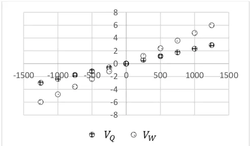
(5) Figure 4 is the comparison diagram that compares 𝑽𝑸 and

𝑽𝑾 to (∆𝟐− ∆𝟏). It shows that 𝑉𝑊’s slope is larger than

𝑉𝑄’s , which represents the range of 𝑉𝑊’s change is larger than 𝑉𝑄’s.

Fig. 4. The comparison diagram that compares 𝑽𝑸 and 𝑽𝑾 to

(∆𝟐− ∆𝟏)

IV. CONCLUSION

In the competitive global market, both pricing strategy and the quality often determine the orientation of the customers. Lowering the price is not a good strategy for the suppliers, it might decrease profit or increase defective products. Therefore, a well-designed quantity discount policy is crucial. This research incorporated quantity discount, unreliable process and uncertain environments into integrated inventory model. Through the sensitive analysis in this study, it shows that if (∆2− ∆1) increases, both 𝑉𝑄 𝑎𝑛𝑑 𝑉𝑊 will increase as well. Also the smaller (∆2+ ∆1) is in the fuzzy model, the more similar it gets to the tradition model. In future, studies may include more manufacturers, then production scheduling will be added into the model to simulate a more realistic situation.

REFERENCES

[1] M.F. Yang, Y. Lin*, W.F. Kao and L.H. Ho (2016, Mar). An Integrated Multi-echelon Logistics Model with Uncertain Delivery Lead Time and Quality Unreliability, Mathematical Problems in Engineering DOI: 10.1155/2016/8494268

[2] Hsin-I Hsiao, Mengru Tu*, M.F. Yang, Wei-Chung Tseng (2017, Jul), "Deteriorating inventory model for Ready-to-eat food under fuzzy environment," International Journal of Logistics Research and Applications (Accepted, Article in press). DOI: 10.1080/13675567.2017.1351532

[3] C.Y. Chiu,Y. Lin, and M.F.Yang (2014, Jul). Applying Fuzzy Multi objective Integrated Logistics Model to Green Supply Chain Problems. Journal of Applied Mathematics, Volume 2014, Article ID 767095, 12 pages. (SCI, 104/247,MATHEMATICS, APPLIED ). NSC 100-2410-H-019-004.

[4] M.F. Yang*, T.S. Huang and Y. Lin,” Variable lead time fuzzy inventory system under backorder rate with allowed shortage”, International Journal of Innovative Computing Information and Control, Vol.6 (2010), No. 11, 5015-5034.

[5] Ben-Daya, M. and M. Hariga, 2000. Economic lot scheduling problem with imperfect production process. Journal of the Operational Research Society, 51:875-881. DOI: 10.1057/palgrave.jors.2600974.

[6] Chakravarty, A.K. and G.E. Martin, 1988. An optimal joint buyer-seller discount pricing model. Computers and Operations Research, 15:271-281.

[7] Huang, C.K., 2004. An optimal policy for a single vendor single-buyer integrated production-inventory. problem with process unreliability consideration. Int. J. Product. Econom., 91: 91-98. DOI: 10.1016/S0925-5273(03)00220-2

[8] Li, J. and L. Liu, 2006. Supply chain coordination with quantity discount policy. Int. J. Product. Econom., 101: 89-98. DOI: 10.1016/j.ijpe.2005.05.008

[9] Lin, Y.J. and C.H. Ho, 2011. Integrated inventory model with quantity discount and price-sensitive demand. TOP, 19: 177-188. DOI: 10.1007/s11750-009-0132-1

[10] Porteus, E.L., 1986. Optimal lot sizing, process quality improvement and setup cost reduction. Operat. Res., 34: 137-144. DOI: 10.1287/opre.34.1.137

[11] Salameh, M.K. and M.Y. Jaber, 2000. Economic production quantity model for items with imperfect quality. Int. J. Product. Econom., 64: 59-64. DOI: 10.1016/S0925-5273(99)00044-4

[12] Schwaller, R.L., 1988. EOQ under inspection costs. Product. Inventory Manage., 29: 22-24.

[13] Wang, Q., 2005. Discount pricing policies and the coordination of decentralized distribution systems. Decision Sci., 36: 627-646. DOI: 10.1111/j.1540-5414.2005.00105.x

[14] Zhang, Z. and J. Xu, 2014. Applying nonlinear MODM model to supply chain management with quantity discount policy under complex fuzzy environment. J. Indust. Eng. Manage., 7: 660-680. DOI: 10.3926/jiem.1079

[15] J. S. Yao and K. Wu (2000), Ranking fuzzy numbers based on decomposition principle and signed distance, Fuzzy Sets and Systems, Vol. 116, pp. 275-288

[16] A. Kaufmann and M. M. Gupta (1991), Introduction to Fuzzy Arithmetic: Theory and Applications, Van Nostrand Reinhold, New York.

[17] H. J. Zimmermann (1996), Fuzzy Set Theory and its Application, 3rd edition, Kluwer Academic Publishers, Dordrecht.

[18] Lal, R. and R. Staelin, 1984. An approach for developing an optimal 145000

150000 155000 160000 165000 170000

-1500 -1000 -500 0 500 1000 1500

E

K(

$

)

-8 -6 -4 -2 0 2 4 6 8

-1500 -1000 -500 0 500 1000 1500

[image:5.595.45.293.603.747.2]

discount pricing policy. Manage. Sci., 30: 1524-1539. DOI: 10.1287/mnsc.30.12.1524