AutoBayes: A System for Generating Data
Analysis Programs from Statistical Models
BERND FISCHER and JOHANN SCHUMANN RIACS / NASA Ames, Moffett Field, CA USA (e-mail:{fisch,schumann}@ptolemy.arc.nasa.gov)
Abstract
Data analysis is an important scientific task which is required whenever information needs to be extracted from raw data. Statistical approaches to data analysis, which use methods from probability theory and numerical analysis, are well-founded but difficult to imple-ment: the development of a statistical data analysis program for any given application is time-consuming and requires substantial knowledge and experience in several areas.
In this paper, we describe AutoBayes, a program synthesis system for the
genera-tion of data analysis programs from statistical models. A statistical model specifies the properties for each problem variable (i.e., observation or parameter) and its dependencies in the form of a probability distribution. It is a fully declarative problem description,
similar in spirit to a set of differential equations. From such a model,AutoBayes
gen-erates optimized and fully commented C/C++ code which can be linked dynamically into the Matlab and Octave environments. Code is produced by a schema-guided deduc-tive synthesis process. A schema consists of a code template and applicability constraints which are checked against the model during synthesis using theorem proving technology.
AutoBayes augments schema-guided synthesis by symbolic-algebraic computation and
can thus derive closed-form solutions for many problems. It is well-suited for tasks like
esti-mating best-fitting model parameters for the given data. Here, we describeAutoBayes’s
system architecture, in particular the schema-guided synthesis kernel. Its capabilities are illustrated by a number of advanced textbook examples and benchmarks.
1 Introduction
In this paper, we describe AutoBayes, a program generator for scientific data analysis programs.
Scientific data analysis is usually based on statistical methods. The expected properties of the data are described in the form of a statistical model: for each problem variable (i.e., observation or parameter), properties and dependencies are specified via probability distributions. In many applications, an initial statistical model of the data is readily available, but the parameters of the model (e.g., mean values and variances) are unknown. Then, a typical data analysis task is to fit observed data against the model, i.e., to find the best possible or most likely values of the unknown parameters under the constraints specified by the model. Here we concentrate on generating programs for suchparameter learning tasks.
AutoBayesstarts from a very high-level description of the data analysis prob-lem in the form of such a statistical model and generates imperative programs through a schema-based deductive synthesis process. A schema is a code template with associated semantic constraints which define and restrict the template’s appli-cability. The schemas are applied recursively to the entire problem or subproblems. AutoBayesaugments this schema-based approach by symbolic-algebraic calcula-tion and simplificacalcula-tion to derive closed-form solucalcula-tions for the entire problem (or subproblems) whenever possible. This is a major advantage over other statistical data analysis systems which have to use slower and possibly less precise numerical approximations even in cases where closed-form solutions exist. The backend of AutoBayes is designed to support generation of code for different programming languages and different target systems. Our current version generates C/C++ code which can be linked dynamically into the Octave or Matlab environments; other target systems can be added easily.
classes
N
σ
µ
gauss
c
N
pointsdiscrete
x
N
classes [image:3.612.190.407.142.287.2]φ
Fig. 1. Bayesian network for the mixture of Gaussians example
very low ozone readings, thus delaying the detection of the ozone hole over the Antarctic by several years (Centre for Atmospheric Science, 1999). Automated pro-gram synthesis can help to solve such problems. It encapsulates a considerable part of the required expertise and allows the developers to program in models, thereby increasing their productivity. By automatically generating code from these models, many programming errors are prevented and turn-around times are reduced.
This paper is an extended version of (Fischeret al., 2000); design rationales and some preliminary results of the AutoBayes-project have also been reported in (Buntineet al., 1999). Section 2 contains a very short introduction into probabilis-tic and graphical reasoning; we refer to the cited literature for more information. Section 3 explains the mixture of Gaussians model in more detail; that model is used as the running example throughout this paper. We then proceed in Sections 4 and 5 with a detailed description of the system architecture and the code synthesis process. Section 6 illustrates in detail the derivation of code for the running ex-ample; it also contains an overview of a number of other example problems solved byAutoBayes. We compare our approach to related work in Section 7 before we concluded and discuss future work in Section 8.
2 Probabilistic and Graphical Reasoning
Graphical models such as Bayesian networks are a common representation method in machine learning and statistical data analysis (Pearl, 1988; Buntine, 1994; Frey, 1998; Jordan, 1999). They combine probability theory and graph theory. From a computational point of view, their appeal is that they can replace some expensive probabilistic reasoning by faster graphical reasoning.
nodes can represent discrete as well as continuous random variables; these are usu-ally represented by boxes and circles, respectively. In the example, c is the single discrete random variable while µ, σ, φ, andxare all continuous random variables. Shaded nodes represent known variables, i.e., input data; here, onlyxis known. Dis-tribution information for the random variables is attached to the respective nodes; here,xis distributed as a Gaussian. Lightly shaded boxes enclosing a set of nodes represent vectors of independent, co-indexed random variables. In the example, µ andσare both vectors of sizeNclasses which always occur indexed in the same way. As a consequence, a box around a single node represents the familiar concept of a vector of independent and identically distributed variables.
The edges in a Bayesian network can sometimes be interpreted as causal influence links between the respective variables. For example, the edge fromµtoxrepresents the influence the (hypothetical) choice of µ has on the observed data x. More precisely, however, the edges encode a conditional independence relationship: each node is independent of its ancestors given its parents. In the example, xis thus independent of φgivenc, µ, andσ. Consequently, the conditional probabilityP(x| c, φ, µ, σ) is equal to—and can thus be simplified to—P(x|c, µ, σ). The network thus superimposes a structure on the global joint probability distribution which can be exploited to optimize probabilistic reasoning. Hence, the example defines the joint probabilityP(x, c, φ, σ, µ) in terms of simpler probabilities:
P(x, c, φ, σ, µ) =P(φ)·P(c|φ)·P(µ)·P(σ)·P(x|c, µ, σ)
Probabilistic reasoning is currently subject to a—sometimes heated—debate be-tween two different schools of thought, the so-called “frequentist” and “Bayesian” approaches. The basic difference between the two approaches is their view of prob-ability. In the frequentist approach, a probability is viewed as a relative frequency which is the outcome of a long series of repeated identical experiments. In a strict-ly frequentist sense no inference can thus be made based on single events. In the Bayesian approach, a probability is viewed as a degree of belief that an event oc-curs. Prior beliefs and knowledge of the state of the analyzed system are specified by prior distributions or priors for short. New data is then considered evidence which is combined with the priors, usingBayes rule
P(h|d) = P(d|h)·P(h) P(d)
Theposterior probability P(h|d) that the hypothesishholds under the new data d is thus expressed in terms of the likelihood P(d| h) and the prior P(h); the probability of the data,P(d), is a normalizing constant. Despite these fundamental differences in interpretation, the techniques applied in both approaches are quite similar. A frequentist analysis can usually be simulated in the Bayesian approach by choosing an appropriate non-informative prior, or, intuitively, by leaving the model parameters uninterpreted. AutoBayes can thus be used as a tool in both approaches; the preference for a particular approach is reflected in the formulation of the statistical model only.
prob-(a)
290.5 291 291.5 292
0 500 1000 1500 2000
binding energy [eV]
measurement no data points (b) 0 10 20 30 40 50 60 70 80 90 100
289 289.5 290 290.5 291 291.5 292 292.5 293
rel. density
binding energy [eV]
data class 1 0 10 20 30 40 50 60 70 80 90 100
289 289.5 290 290.5 291 291.5 292 292.5 293
rel. density
binding energy [eV]
data class 1 class 2 0 10 20 30 40 50 60 70 80 90 100
289 289.5 290 290.5 291 291.5 292 292.5 293
rel. density
binding energy [eV]
data class 1 class 2 class 3
Fig. 2. (a) Artificial input data for the mixture of Gaussians example: 2400 data points
in the range [290.2,292.2]. Each point belongs in one of three classes which are Gaussian
distributed withµ1 = 290.7, σ1 = 0.15,µ2 = 291.13, σ2 = 0.18, andµ3 = 291.55, σ3 =
0.21. The relative frequenciesφfor the points belonging to the classes are 61%,33%, and
6%, respectively. (b) Histogram (spectrum) of the artificial test data from (a) and Gaussian distributions which are obtained as the result of the synthesized data analysis program.
lems. In the first case, parameter learning, both data and model are given and the parameters of the model (in our example µ, σ, and φ) have to be determined. In the second case, structure learning, only the data is given, and both the model and its parameters have to be determined. This involves a usually heuristic search in the space of all models, e.g., using a hill climbing method. Within this search, parameter learning usually re-appears as a subtask. Currently, AutoBayesis set up to handle parameter learning only—it requires the (parameterized) model spec-ification as input. However, it can in principle also be employed in the inner loop of a structure learning algorithm.
Parameter learning is basically an optimization problem. In some cases, closed form solutions for the optimal parameter values exist and the equations derived from the network structure and the probability density functions can be solved symbolically. In general, however, iterative methods must be applied to solve the optimization problem. Typically, learning and classification algorithms as for ex-amplek-Meansorexpectation maximization (EM)are used. For some subproblems, classical numerical optimization algorithms like Newton, Gauss-Newton, or other variants are applicable.
3 An Example: Mixture of Gaussians.
Throughout this paper, we will illustrate how AutoBayes works by means of a simple but realistic classification example. Figure 2(a) shows the raw input data, a vector of real values. We know that each data point falls into one of three classes; each class iis Gaussian distributed with mean µi and standard deviation σi. The data analysis problem is to infer from the given data the relative class frequen-cies φi (i.e., how many points belong to each class) and the unknown distribution parameters µi andσi for each class.
[image:5.612.118.470.144.250.2]1 model mog as ’Mixture of Gaussians’; 2
3 const int n_points as ’number of data points’
4 with 0 < n_points;
5 const int n_classes := 3 as ’number of classes’
6 with 0 < n_classes
7 with n_classes << n_points;
8
9 double phi(0..n_classes - 1) as ’class probabilites’
10 with 1 = sum(I := 0..n_classes - 1, phi(I));
11 double mu(0..n_classes - 1), sigma(0..n_classes - 1);
12
13 int c(0..n_points) as ’class assignment vector’;
14 c ~ discrete(vec(I := 0..n_classes - 1, phi(I)));
15
16 data double x(0..n_points - 1) as ’data points (known)’;
17 x(I) ~ gauss(mu(c(I)), sigma(c(I)));
18
19 max pr(x | {phi, mu, sigma}) wrt {phi, mu, sigma};
Fig. 3. AutoBayes-specification for the mixture of Gaussians example. Line numbers
have been added for reference in the text. Keywords are underlined.
describes an application in physics where gas atoms (or molecules) are excited with a specific energy (e.g., light from a laser). They can then absorb this energy by excitation or electron emission. This basic mechanism generates spectral lines like those observed in the light of stars. Single atoms usually have sharp, well-defined spectral lines but the more complex molecules (e.g., CH4 or NH3) can have several peaks of binding energy, depending on their internal configuration. Thus, they can absorb (or emit) energy at different levels. Figure 2(b), which is adapted from (Berkowitz, 1979), shows an spectrum of the energy of emitted photoelectrons which is directly related to the excess energy of photons over the photoionization potential of CH4molecules (for details see (Berkowitz, 1979), caption of Figure 67). Since CH4 which has three internal distinct configurations, the spectrum shows three distinct peaks.
In a simple statistical model, each of the peaks is assumed to be independently Gaussian distributed and the percentage of molecules in a specific configuration is assumed to be known. When we measure the binding energies for a large number of CH4 molecules (with unknown internal configurations), we obtain a data set similar to the one shown in Figure 2(a). We can then use a program implementing the statistical model to classify the data points into the three classes and to obtain the parameters. Figure 2(b) shows the histogram of the data, superimposed with Gaussian curves using the parameter values estimated by the program generated byAutoBayes.
Figure 3 shows the detailed statistical model for this problem in AutoBayes’s specification language. The model (called “Mixture of Gaussians” – line 1) as-sumes that each of the data points (there are n points– line 5) belongs to one of
left unspecified. Lines 16 and 17 declare the input vector and distributions for the data points.1 Each point x(I) is drawn from a Gaussian distribution c(I) with
mean mu(c(I))and standard deviation sigma(c(I)). The unknown distribution
parameters can be different for each class; hence, we declare these values as vectors (line 11). The unknown assignment of the points to the classes (i.e., distributions) is represented by the hidden (i.e., not observable) variable ccorresponding to the internal configuration of the molecule. The class probabilities or relative frequencies are given by the also unknown vector phi (lines 9–14). Since each point belongs to exactly one class, the sum of the probabilities must be equal to one (line 10). Additional constraints (lines 4, 6, 7) express further basic assumptions of the mod-el. Finally, we specify the goal inference task (line 19), maximizing the conditional probabilitypr(x | {phi, mu, sigma})with respect to the parameters of interest,
phi,mu, andsigma. This means, we are interested in obtaining the values for the model parameters which best fit the given data.
This classification problem is a typical task in (unsupervised) machine learning for which a variety of algorithms and approaches exist (see, e.g., (Mitchell, 1997; Bishop, 1995)).AutoBayes currently implements two such algorithms which are known in the literature as k-Means and expectation maximization or simply EM algorithm(Dempsteret al., 1977; McLachlan & Krishnan, 1997), respectively. Both algorithms are applicable to a variety of mixture models (McLachlan & Peel, 2000) which underpin many classification tasks similar to our running example.
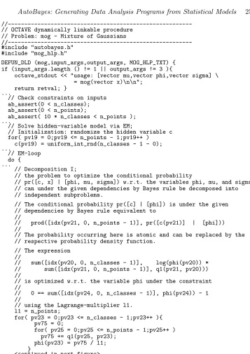
The EM-algorithm is an iterative numerical algorithm which applies to maximiza-tion tasks of the form maxP(U|V)wrtV, given a setW ofhidden variables. In our example,U ={x},V ={phi, mu, sigma}, andW ={c}. The algorithm basically consists of three steps; the first step performs initializations. In our implementa-tion, the initialization just “guesses” values for the hidden variables by performing random assignments. These assignments are made to a matrix qwhere q(i,j) is the probability that pointibelongs to classj. Then an iteration is performed over the remaining two steps, the expectation or E-step, and the maximization or M -step. This iteration is performed until the changes of the involved variables become sufficiently small. During the iteration, E-step andM-step change the position of the distribution parameters.
• M-step: given the current distribution ofW (in our example, the values of the matrixq and the dataU), new values for the distribution parameters V are estimated by maximizingP({W, U} |V) with respect to V. In our example, this maximization results in new estimates ofmu and sigma for each of the classes.
• E-step: given the current estimated values for the distribution parametersV and the dataU, the probability distribution ofW is calculated. In the discrete case, as in our example, this distribution can be obtained relatively easily by summing up over the domain ofW. Thus, in our case, we update the matrix
qto reflect the new estimates of the parameters.
1
The individual steps of this generic algorithm need to be adapted for the specific model. For example, the maximization step requires information about the distri-bution of all variables and involves substantial symbolic calculations (e.g., as shown in the for-loop near the bottom of Figure 7).
4 System Architecture
4.1 Overview
AutoBayes’s overall system architecture is shown in Figure 4. In a first process-ing step, the given specification is parsed and converted into internal form and the Bayesian network is constructed. This step can also generate an external represen-tation for visualization purposes, using thedot graph drawing tool (Koutsofios & North, 1996). The synthesis kernel, which will be described in detail in Section 5, then analyzes the network, tries to solve the given optimization task, and instan-tiates appropriate algorithm schemas which are given in a schema library. The output of the synthesis kernel is a program in a procedural intermediate language. AutoBayes’s backend (see Section 4.2) takes this intermediate code, optimizes it and generates code for the chosen target system. Currently, we target Octave and Matlab but only small parts of the code generator are system-specific; new target systems can thus be added easily. The synthesis kernel also produces detailed doc-umentation along with the code (see Section 4.3). Furthermore, AutoBayescan generate code which generates artificial data for the model, e.g., for visualization and testing purposes (see Section 4.4).
All parts of the AutoBayes system rely heavily on a symbolic subsystem and some auxiliary system modules (e.g., pretty-printer, set representations, I/O func-tions). For symbolic mathematical calculations, we implemented a small but reason-ably efficient rewriting engine in Prolog. Graph handling, simplification of math-ematical expressions, and an equation solver are implemented on top of it. The system architecture is designed in such a way that most of its parts can be re-used in different domains. In particular, backend and symbolic subsystem are entirely independent of the data analysis domain. The entire system has been implemented in SWI-Prolog (Wielemaker, 1998) and comprises about 31,000 lines of documented Prolog code. Since AutoBayes requires a combination of sound symbolic math-ematical calculation, rewriting, and general purpose operations (e.g., output to multiple files, handling of strings, interface to the operating system), Prolog is a reasonable choice as the underlying implementation language. SWI-Prolog proved to be a very stable and efficient development platform with reasonable debugging facilities.
4.2 Generating Code
...
n_points n_classes n_classes
c discrete
x Gaussian rho sigma mu
for(i=0;i<n.. Input Parser
Optimizer
Code Generator Synthesis Kernel Test-data
Generator
AutoBayes Specification
intermediate code
System
utilities
Rewriting Engine Simplifier Equation Solver
Library Schema
C/C++ code X ~gauss(mu,..
Visualization
internal repr. of spec
[image:9.612.131.467.140.482.2]simple proc. language simple proc. language
Fig. 4. System architecture ofAutoBayes.
assertions and annotations. The intermediate language is still close enough to the current target languages (i.e., C and C++) such that the translation down into the chosen target language remains simple. The domain-specific constructs allow target-specific optimizations and transformations. For example, the sum-construct of the intermediate language for calculating the sum of array elements can be con-verted into a usual for-loop, an iterator construct for sparse matrices, or a direct call to a summation-operator (e.g., when generating interpreted Matlab code).
expres-sions) are left for the subsequent compilation phase—there is no need to perform the same optimization steps as any modern compiler.
The currentAutoBayes-version generates C++-code for Octave (Murphy, 1997), C-code for Matlab (Moler et al., 1987), and stand-alone C-code. Future work will include code-generators for CASE-tools for embedded systems, e.g., ControlShell (ControlShell, 1999) or MatrixX (AutoCode, 1999).
4.3 Generating Documentation
Certification procedures for safety-critical applications (e.g., in aircraft or space-craft) often mandate manual code inspection. This inspection requires that the code is readable and well documented. Even for programs not subject to certifica-tion, understandability is a strong requirement as manual modifications are often necessary, e.g., for performance tuning or system integration. However, existing program generators often produce code that is hard to read and understand. In order to overcome this problem, AutoBayes generates explanations along with the programs which show the “synthesis decisions”: which algorithm schema has been used, how the schema parameters have been instantiated, etc. Used model as-sumptions and proof obligations that could not be discharged during the synthesis are laid out clearly. This makes the synthesis process more transparent and provide traceability from the generated program back to the model specification.
AutoBayesgenerates extensively commented code: approximately one third of the output lines are automatically generated comments (cf. Figure 7 for an ex-ample). This is achieved by embedding documentation templates into the code templates. Future versions ofAutoBayeswill not only generate fully documented code; we aim to produce a detailed standardized design-document for the generated code.
4.4 Generating Artificial Test Data
Visualization and simulation plays an important role in the development of data analysis programs. AnAutoBayes model specification contains enough informa-tion to synthesize code which generates artificial data according to the specificainforma-tion. For example, the data set in Figure 2(a) has been generated that way. Generating artificial test data is very helpful in understanding the model and the generated code. If the artificial data does not match real data sets (or the scientist’s expecta-tions), the specified model might not reflect the reality properly. Artificial data sets can also be used to assess and evaluate the performance of the synthesized code before real data becomes available. This feature is of particular interest in cases where the domain theory allows instantiation of different algorithms for the same specification. For example, ifAutoBayessynthesizes different variants for initial-ization of the hidden variable, their coarse relative performance can be assessed with the generated test data.
is exactly the same as for the synthesis of the data analysis program. This data generator was implemented in less than 200 lines of Prolog code on top of the AutoBayessystem.
5 The Synthesis Kernel
5.1 Network Construction
The synthesis kernel takes the internal representation of the model specification and builds an initial Bayesian network. Each variable declaration in the model corresponds directly to a network node. Each distribution declaration of the form x∼D(Θ) (for any distributionD) induces edges from the distribution’s parameters Θ to the node corresponding to the random variablex; these edges reflect the de-pendency of the (random) values ofxon the values of the parameters Θ. Building the network is relatively straight-forward and requires no sophisticated dataflow analysis because the model is purely declarative. However, Θ needs to be flattened, i.e., nested random variables need to be lifted and fresh index variables need to be introduced in their place in order to represent the dependencies properly. Hence, the example declarationx(I) ~ gauss(mu(c(I)), sigma(c(I)))induces not on-ly the two obvious edges but three:mu(J)−→x(I),sigma(J)−→x(I), andc(I)
−→x(I) (cf. Figure 1). Note thatxandcare still co-indexed but that eachx(I)
now depends on all mu(J) and sigma(J), reflecting the unknown values of their original indices c(I). A compact representation of the indexed nodes and their dependencies is achieved by using Prolog-variables to represent index variables.
5.2 Schema-Guided Synthesis
Synthesis proceeds from this initial network and the original probabilistic inference task by exhaustive application ofschemas. A schema can be understood as an “in-telligent macro”: it comprises apattern, aparameterized code template, and a set of preconditions or applicability constraints. The pattern and code template are simi-lar to the left- and right-hand side of a traditional macro definition; they comprise the syntactic part of the schema. Schema-guided synthesis, however, is not just macro expansion. Different schemas can match the same pattern, possibly in differ-ent ways. During synthesis, these schemas are tried exhaustively in a left-to-right, depth-first manner. Whenever a dead end is encountered (i.e., no schema is applica-ble),AutoBayesbacktracks. This control regime allowsAutoBayesto generate code as a composition of different schemas, thus “re-inventing” data-analysis al-gorithms from simple building-blocks. Furthermore, backtracking in AutoBayes results in the synthesis of program variants if multiple schemas are applicable and thus yields the capability to generate multiple solutions for the same problem.
parameters further. The search process mentioned above is thus a proof search; the proof is constructive in the sense that it actually generates a program (thewitness) and does not just assert its existence.
Network decomposition schemas. AutoBayes uses four different kinds of schemas.Network decomposition schemas are encodings of independence theorems for Bayesian networks (see for example (Pearl, 1988)). They describe how a prob-abilistic inference task over a given network can be decomposed equivalently into simpler tasks over simpler networks and, hence, how a complex data analysis pro-gram can be composed from simpler components. The applicability constraints for these schemas can be checked by pure graph reasoning. Consider for example the following decomposition theorem:
Let U, V be sets of vertices in a Bayesian network such that U ∩V =∅. Then V ∩descendants(U) =∅ andparents(U)⊆V implies
P(U|V) = P(U|parents(U))
= Q
u∈UP(u|parents(u))
This theorem allows us to simplify the conditional probability P(U | V) into P(U|parents(U)). This means that we can safely ignore all assumptions not re-flected in the network by incoming edges. Then P(U|parents(U)) can further be decomposed into a finite product of atomic probabilities (i.e., each variable de-pends only on the parameters of its associated distribution), provided that the applicability constraints hold over the network; here,descendants(U) is the set of all nodes (directly or indirectly) reachable from nodes in U excluding U. Within AutoBayes, this theorem is implemented by the following network decomposition schema for maximizing the probability P(U|V) with respect to a set of variables X:
schema(max P(U|V) wrt X,Template )
:-U∩V =∅
∧ V ∩descendants(U) =∅ ∧ parents(U)⊆V ∧ . . . →Template= begin
h∀u∈U : max P(u|parents(u)) wrt (X∩parents(u)i
end
In our ongoing example, this decomposition schema is applied when the interme-diate goal max pr({c, x} | {phi, mu, sigma}) wrt {phi, mu, sigma} is pro-cessed. WithU ={c, x},V ={phi, mu, sigma}, and X ={phi, mu, sigma}, it is easy to see that all requirements for the schema are satisfied (see Figure 1 for the dependencies among the variables). Thus, we obtain the following two (sim-pler) maximization goals:max pr(c | phi) wrt {phi}, andmax pr(x | {c, mu,
sigma}) wrt {mu, sigma}.
A number of similar decomposition theorems have been developed in probabil-ity theory; AutoBayes currently includes three different schemas based on such theorems, with the one shown above being by far the simplest. For details on the other schemas see (Buntine et al., 1999).
Formula decomposition schemas. Formula decomposition schemas are similar to the network decomposition schemas above but they work on complex formulae instead of a single probability. The following schemas are typical members of this class.
• Index decompositionapplies to an inference task for a formula which contains multiple occurrences of probabilities involving vectors and “unrolls” this task into a loop over the simpler inference task for a single vector element. In our example, one subtask is max pr(x | {c, mu, sigma}) wrt {mu, sigma}. Since the vectorx is independently and identically distributed (i.e., has the same distribution for each data point), maximization can be done separately for eachI. Thus, we obtain the code fragmentfor i=0..n points-1 : hmax
pr(x(I) | {c(I), mu, sigma}) wrt {phi(i)}i.
• Split/back-substitute splits a mixed discrete-continuous maximization prob-lem into two separate discrete and continuous subprobprob-lems, respectively, and substitutes a symbolic solution of the continuous subproblem back into the discrete subproblem.
• Iterate-range: solves a discrete maximization problem by iteration over the finite range of the variables.
Most of the applicability constraints for these decomposition schemas can still be checked by graph reasoning but some checks involving the formula structure require substantial symbolic reasoning.
Statistical algorithm schemas. Proper statistical algorithm schemas are also graph-based but they are not simple consequences of the independence theorems. These schemas involve larger modifications of the graph, e.g., introduction of new nodes with known values, and storing the results of intermediate calculations. These schemas thus enable the further application of the decomposition schemas; however, they are much more intricate and less theorem-like. Hence, their correctness is proven independently, or they are just empirically validated during construction of the domain theory. Statistical algorithm schemas also have much larger and usually iterative code templates associated with them and they can require substantial symbolic reasoning during instantiation. AutoBayes currently implements two such algorithms, namelyk-Means and theEM algorithm.
maxi-mization tasks of the form max P(U|V)wrt V, given a setW ofhidden variables. WithinAutoBayes, EM is encoded as the following schema:
schema(max P(U|V) wrt V,Template )
:-. :-. :-.
→Template= begin
Initialize: guess values forW
while-converging(V)
M-step:max P({W, U}|V)wrt V E-step: calculateP(W|{U, V})
end end
Each of the three steps (initialization,M-, andE-step) cause recursive calls to the synthesizer. The maximization task in theM-step triggers further decompositions by the assumption that the hidden variables W are now known.
Numerical algorithm schemas. The graph-based reasoning continues until all conditional probabilities P(U | V) have been converted into atomic form, i.e., parents(U) =V. This means that all random variables occurring in the parameters of U’s (joint) distribution are known. Such probabilities can thus be replaced by the appropriately instantiated probability density functions.AutoBayes’s domain theory contains rewrite rules for the most common probability density functions. In our example,pr(x(i) | {mu(j), sigma(j)} is rewritten into
(√2πsigma(j))−1 exp((x(i)−mu(j))2
−2sigma(j)2)
thus instantiating the usual formula for Gaussian distributions. Density functions for problem-specific distributions can easily be defined as part of an AutoBayes specification.
With this elimination step the original probabilistic inference task becomes a pure optimization problem which can be solved either symbolically or numerical-ly. AutoBayes first attempts to find closed-form symbolic solutions, which are much more time-efficient during run-time than iterative numeric approximation al-gorithms. In order to solve the optimization problem, AutoBayes symbolically differentiates the formula with respect to the optimization variables, sets the re-sult to zero and tries to symbolically solve this system of simultaneous equations. Symbolic differentiation is implemented as a term rewrite system; however, some variable dependency checks require conditional rewrite rules. For example, it has to be checked whether the dependent variable of the derivative occurs in a term or not. Equation solving currently employs only a variant of Gaussian variable elimi-nation; whenever a variable can be isolated modulo the symbolic model constants, the remaining equation is solved by a polynomial solver.
reuse typical for libraries. It can instantiate actual parameters symbolically and evaluate the inlined expressions partially. This provides further optimization op-portunities, often in the inner loops of the algorithms. Moreover, symbolic and numeric methods complement each other well. While for many more complex mod-els nocomplete closed-form solutions exist,AutoBayescan usually solve for some variables symbolically. These variables can then be split away from the optimization problems such that the iterative numeric methods need to be applied only to the smaller remaining problems.
Assumptions and Proof Obligations. During symbolic calculation in the syn-thesis kernel, a number of soundness assumptions may accumulate. For example, the expression x/xcan be simplified to 1 only if x6= 0 can be shown. Other as-sumptions stem from the specification or from the applied schemas. Asas-sumptions that cannot be discharged during synthesis are brought to the user’s attention. Assumptions which can be checked efficiently during run-time are converted in-to assertions which are then inserted inin-to the synthesized code (e.g., x 6= 0 or
n classes n points). This approach ensures soundness and reliability of the
generated code.
6 Examples and Results
6.1 Mixture of Gaussians
In this section, we discuss synthesis and execution of the example described in Sec-tion 3. The specificaSec-tion shown in Figure 3 already comprises the entire input to AutoBayes. After parsing the specification,AutoBayesgenerates the dependen-cy graph (cf. Figure 1) and tries to decompose the original goal
max pr(x | {phi, mu, sigma}) wrt {phi, mu, sigma}
into independent parts. In this case, however, the graph is not directly decompos-able, and the system tries the match and instantiate one of the statistical algorithm schemas. Here, the EM-schema is applicable and the system identifiescas the single hidden variable, i.e.,W ={c}. For representation of the distribution of the discrete hidden variablec, a matrix qis generated, where q(I, J) is the probability that thei-th point falls into thej-th class. This array is then initialized using random values. The E-step essentially yields a discrete distribution
c(I) ~ discrete(vec(J := 0..n classes - 1, q(I, J))
For theM-step,AutoBayesis recursively called with the new goal
max pr({c, x} | {phi, mu, sigma}) wrt {phi, mu, sigma}
Now, the network decomposition schema described in Section 5.2 applies withU =
{c, x},V ={phi, mu, sigma}, andX ={phi, mu, sigma} which spawns two
new subgoals. The first subgoal
can be unrolled over the independent and identically distributed vectorc, using an index decomposition schema:
max Qn classes−1
I:=0 pr(c(I) | phi) wrt {phi}
This yields a constrained maximization problem in the vectorphi(cf. the constraint
with 1 = sum(I := 0..n classes - 1, phi(I)) in line 10 of the specification)
which is solved by an application of the Lagrange multiplier schema. This in turn results in two subproblems for a single instancephi(j)and for the multiplier which are both solved symbolically. The detailed formulas can be found in Figure 7 near
Decomposition I.
The second subgoal from the decomposition schema,
max pr(x | {c, mu, sigma}) wrt {mu, sigma}
can be unrolled in a similar fashion but since c and x are co-indexed, unrolling proceeds over both (also independent and identically distributed) vectors in parallel:
max Qn points−1
I:=0 pr(x(I) | {c(I), mu, sigma}) wrt {mu, sigma}
The probabilitypr(x(I) | {c(I), mu, sigma})is atomic becauseparents(x(I))
= {c(I), mu, sigma}. It can thus be replaced by the appropriately instantiated
Gaussian density function:
max Qn points−1 I:=0 (
√
2πsigma(c(I)))−1 exp((x(I)−mu(c(I)))2
−2sigma(c(I))2) wrt {mu, sigma}
The next step is to “wrap” a log around the formula. This does not change the maximizing values because log is a strictly monotone function, but it makes the maximization problem easier.
max Pn points−1 I:=0
(x(I)−mu(c(I)))2
−2sigma(c(I))2 −log √
2π−logsigma(c(I))
wrt {mu, sigma}
Now, the hidden variablecis marginalized using the distribution calculated in the E-step. This is accomplished here by summing over the domain of ]tt c, i.e., all possible classes.
max Pn points−1 I:=0
Pn classes−1 J:=0 q(I,J)
(x(I)−mu(J))2
−2sigma(J)2 −log √
2π−logsigma(J)
wrt {mu, sigma}
This numerical optimization problem for the whole vectors mu and sigma is then simplified by another application of the index decomposition schema into a sub-problem for two single instances mu(J) and sigma(J); the fact that both vectors can be unrolled in parallel is again a consequence of the graph structure. In a last step, Gaussian elimination is used to solve this subproblem symbolically, yielding an expression to first calculatemu(J)and thensigma(J).
mu(J)=Pn points−1
I:=0 (1/q(I,J))
Pn points−1
K:=0 x(K) q(K,J)
sigma(J)=Pn points−1
I:=0 (1/
p
q(I,J)) Pn points−1
K:=0
p
(a)
n_points
n_classes n_classes
c discrete
x Gaussian phi sigma mu
(b)
1e-04 0.001 0.01 0.1
0 100 200 300 400 500 600 700 800 900 1000
log(Error)
iteration steps
convergence
Fig. 5. (a) Bayesian network for the mixture of Gaussians example, automatically
gener-ated byAutoBayesfrom the textual specification; (b) convergence behavior: differences
between old and new parameters (log-scale) over iteration step. Only the first 1000 itera-tion cycles are shown.
For the entire example,AutoBayessynthesizes a C++ file consisting of 389 lines, including comments and separation lines. A portion of this code is shown in Fig-ure 7. The code is then compiled into a dynamically linkable function for Octave. Thus, when the functionmog (cf. line 1 of the specification) is invoked within the Octave environment, the compiled C++ code is invoked automatically. As shown in a sample run in Figure 6, AutoBayes also synthesizes code to show the re-quired input- and output parameters (“usage”). The entire synthesis process of AutoBayes, including compilation of the generated C++ code takes about 25 secs. on a 400Mhz Sun Ultra 60. For further details, see problemM1in Table 1.
We have tested the synthesized code with artificial test data which has been generated by the test data generator synthesized by AutoBayes from the same model. The data set consists of 2400 points divided into 3 classes (cf. Figure 2). From these inputs, the algorithm searches for the values ofmu,sigma, andphi for each class. The convergence, i.e., the normalized change of the parameters to be optimized during each iteration cycle, is shown in Figure 5. This algorithm does not necessarily converge monotonically. It can reach some local minimum, from which it has to move away by increasing the error again. After some ups and downs the global minimum (i.e., an optimal estimate for the parameters) is reached and the loop ends. This behavior is typical for many iterative parameter estimation processes. In this case, the final result required 1163 iteration steps, taking approximately 48 secs.2 AutoBayes can automatically instrument the generated code to produce these run-time figures for debugging and testing purposes if this is requested via a command line option.
6.2 Other Examples
We have also applied the AutoBayes system to a number of different textbook and benchmark examples. The results of these experiments are shown in Table 1.
2
[image:17.612.118.468.144.251.2]octave:2> mog
usage: [vector mu, vector phi, vector sigma] = mog(vector x)
octave:3> x = [ ... ]; % x contains data to be analyzed
octave:4> [mu,phi,sigma] = mog(x) % call the synthesized code
mu =
291.12 291.28 290.69 ...
Fig. 6. Octave sample session using code (function “mog”) generated byAutoBayes
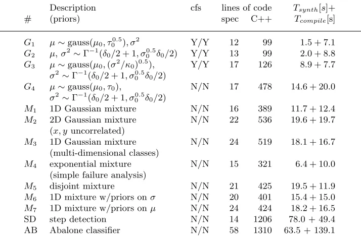
For each problem, a short description of the task or the used priors is given. cfs indicates whether a closed-form solution exists and, if so, whether it has been found by AutoBayes. The next two columns give the size of the specification and the respective number of lines of generated Octave/C++ code, including the automat-ically generated comments. Finally, the synthesis time Tsynth (i.e., AutoBayes’s run-time) as well as the compilation timeTcompile for the GNUg++ compiler (op-timization level-O2) are given. All times are in seconds and have been obtained on a Sun Ultra 60 (400 Mhz) using the Unixtimecommand.
The examplesG1toG4 describe different estimation problems for Gaussian dis-tributions. Given a sample of n data points and various prior information (e.g., the variance of the distribution and an estimate of the mean value), the task is to estimate the remaining parameters of the distribution. For most of these text-book examples closed-form solutions exist (Gelman et al., 1995) and are found by AutoBayes, which demonstrates the capabilities of its symbolic system. The ex-amplesG3andG4also demonstrate how small changes in the specification can lead to dramatically different programs.G3uses the so-called conjugate prior forµand can still be solved in closed form. In G4, however, the slightly more general semi-conjugate prior is used (i.e., the variance of the expected mean is generalized from the form (σ2/κ0)0.5 to a simple variableτ0) which renders the problem unsolvable in closed form and, hence, requires the application of an iterative approximation method, in this case, a Nelder-Mead simplex algorithm.
Description cfs lines of code Tsynth[s]+
# (priors) spec C++ Tcompile[s]
G1 µ∼gauss(µ0, τ
0.5
0 ), σ
2
Y/Y 12 99 1.5 + 7.1
G2 µ,σ 2
∼Γ−
1
(δ0/2 + 1, σ
0.5
0 δ0/2) Y/Y 13 99 2.0 + 8.8
G3 µ∼gauss(µ0,(σ
2
/κ0)0.5
), Y/Y 17 126 8.9 + 7.7
σ2
∼Γ−
1
(δ0/2 + 1, σ
0.5
0 δ0/2)
G4 µ∼gauss(µ0, τ0), N/N 17 478 14.6 + 20.0
σ2
∼Γ−1(δ0/2 + 1, σ
0.5
0 δ0/2)
M1 1D Gaussian mixture N/N 16 389 11.7 + 12.4
M2 2D Gaussian mixture N/N 22 536 19.6 + 19.7
(x, yuncorrelated)
M3 1D Gaussian mixture N/N 24 519 18.1 + 16.7
(multi-dimensional classes)
M4 exponential mixture N/N 15 321 6.4 + 10.0
(simple failure analysis)
M5 disjoint mixture N/N 21 425 19.5 + 11.9
M6 1D mixture w/priors onσ N/N 20 401 15.4 + 15.0
M7 1D mixture w/priors onµ N/N 24 424 18.2 + 16.5
SD step detection N/N 14 1206 78.0 + 49.4
[image:19.612.117.474.132.369.2]AB Abalone classifier N/N 58 1310 63.5 + 139.1
Table 1. List of examples
AutoBayes can easily be extended to handle more complicated mixture mod-els. For example, we have added a higher-order mixture-operator to handle non-parametric mixtures, i.e., models in which the different classes are generated by different probability distribution functions and not only by different parameter val-ues of the same distribution. Themixture-operator simply takes a finite list of the different distributions and mixes them according to the value of the hidden variable, e.g.,
x(I) ~ mixture(c(I) cases
[ 0 -> binomial(m, p), 1 -> poisson(rate) ]);
describes the mixture between a binomial and a Poisson process used in example M5. Due to the schema-based approach, this extension was completely straight-forward and required only two additional Prolog-clauses, one to declaremixtureas the name of a distribution and one to define its distribution function as a cases -construct over the distribution functions of its arguments. In particular, no further functionality specific to the mixture-operator needed to be implemented. Finally, M6 andM7 are one-dimensional mixture examples with prior information (conju-gate prior) on σ and µ, respectively. These examples demonstrate AutoBayes’s capability to synthesize code for classical (i.e., without priors) maximum-likelihood problems as well as for maximum aposteriori (i.e., Bayesian inference) problems.
x(I) ~ gauss(if(I < step, mu1, mu2), sigma);
There are several algorithms for step detection. One of the more common approach-es is the Hinckley-tapproach-est which first finds the maximizing valuapproach-es for mu1, mu2 and
sigmain terms of the still unknown positionstep, substitutes these values back into
the original problem, and then finds the maximizing value for step. AutoBayes “re-invents” this algorithm by composition of three different schemas, a split/back-substitute schema for separating the problem, range-iteration for solving the dis-crete subproblem, and the symbolic solver for handling the continuous part.
The Abalone classification problem AB is a standard machine learning bench-mark from the UCI Machine Learning Repository (Blake & Merz, 1998). Here, the age of an Abalone mussel has to be predicted from a number of physical measure-ments, e.g., its size or weight. Prediction is used because an exact age determination requires an elaborate procedure—cutting the shell, staining it, and counting the number of rings through a microscope. In its original form, the age prediction is a difficult problem because the data set contains only very few entries for very young or very old abalones. It is thus often simplified by partitioning the ages into three roughly equally likely categories “young,” “adult,” and “old.” For this simplified version, AutoBayes generates an unsupervised classifier (i.e., no training phase is required) which is again based on the EM-schema. It achieves a 54.7% accuracy which is only slightly worse than the results of some of thesupervised classifiers.
In general, these results are very encouraging as they indicate thatAutoBayes can already be applied to realistic examples. Except for the last two examples, synthesis times are generally in the sub-minute range; they also compare well with the compile times for the synthesized code. Most of the synthesis time is generally spent in the symbolic subsystem which we believe can still be optimized substan-tially. The only exception here is the step detection exampleSDwhere almost 90% of the synthesis time is spent in the backend. This is a result of the large number of deeply nested summations which are converted into loops and thus require a substantial re-arrangement of the code. In the cases where no closed-form solution exists, the scale-up factor (i.e., the ratio between specification size and code size) is generally around 1:20 which supports our claim that models are much more concise than programs.
We are currently testingAutoBayesin two larger case studies concerning data analysis tasks for finding extra-solar planets, either by measuring dips in the lumi-nosity of stars (Kochet al., 2000), or by measuring Doppler effects (Marcy & Butler, 1997), respectively. Both projects required substantial effort to manually set up da-ta analysis programs. Our goal for the near future is to demonstrateAutoBayes’s capability to handle major subproblems (e.g., the CCD-sensor registration problem) arising in these projects.
7 Related Work
tradition of composing programs from library components but there are only a few, recent attempts to achieve a similar degree of automation as AutoBayes does. The Bayes Net Toolbox (Murphy, 2000) is a Matlab-extension which allows users to program in models; it provides several Bayesian inference algorithms which are attached to the nodes of the network. However, the Toolbox is a purely interpretive system and does not generate programs. The widely used Bugs-system (Thomas et al., 1992) also allows users to program in models but it uses yet another, en-tirely different execution model: instead of executing library code or generating customized programs, it interprets the statistical model using Gibbs sampling, a universal—but less efficient—Bayesian inference technique. Gibbs sampling could be integrated into AutoBayes as an algorithm schema. Mjolsness and Turmon (Mjolsness & Turmon, 2000) recently introduced the concept ofstochastic parame-terized grammars. Such grammars allow a concise model specification in a way very similar to AutoBayes’s specification language. However, they are currently only a notational device without any underlying program execution or synthesis model. Deductive synthesis is still an active research area, despite its long heritage go-ing back to (Green, 1969) and (Waldgo-inger, 1969). Some systems, however, have already been applied to real-world problems. TheAmphionsystem (Stickelet al., 1994) has been used to assemble programs for celestial mechanics from a library ofFortrancomponents, for example the simulation of a Saturn fly-by.Amphion is more component-oriented than AutoBayes, i.e., the generated programs are linear sequences of subroutine calls into the library. It uses a full-fledged theorem prover for first-order logic and extracts the program from the proof. Ellman and Murata (Ellman & Murata, 1998) describe a system for the deductive synthesis of numerical simulation programs. This system also starts from a high-level specifica-tion of a mathematical model—in this case a system of differential equaspecifica-tions—but is again more component-oriented than AutoBayes and does not use symbolic-algebraic reasoning. Planware (Blaine et al., 1998) (which grew out of the Kids system (Smith, 1990)) synthesizes schedulers for military logistics problems. It is built on the concept of an algorithm theory which can be considered as an explicit hierarchy of schemas, but the underlying basic synthesis process is a different one. Biggerstaff (Biggerstaff, 1999) presents a short classification of generator tech-niques (albeit cast in terms of their reuse effects). AutoBayes falls most closely into the category of inference-based generators but also exhibits some aspects of pattern-directed and reorganizing generators, e.g., the typical staging of the schemas into multiple levels.
8 Conclusions and Future Work
an intermediate language, AutoBayesgenerates executable, optimized code for a target system. The current version produces C/C++-code which can be linked dy-namically into the Octave and Matlab environments. We have tested AutoBayes on a variety of text-book and benchmark examples. In most cases, run-time for syn-thesizing code was well below one minute; compiling the synthesized codes takes roughly the same amount of time. The code is well documented and robust.
Although we have been able to generate code for various non-trivial textbook examples, AutoBayes’s capabilities to generate code for a variety of statistical models must be extended, before it can be employed by the working data analyst. We will add further algorithm schemas for statistical algorithms (e.g., variants of the EM-algorithm) and for general numerical optimization to the system. Future versions ofAutoBayeswill also be extended in such a way that statistical models over time series can be handled. Here, we are planning to incorporate specific algo-rithm schemas for handling a restricted but common class of time-series problems as well as standard optimization methods like finite differencing.
AutoBayesoffers several unique features which result from using program syn-thesis instead of compilation and which make it more powerful and more versatile for the application domain than other tools and statistical libraries. AutoBayes can generate efficient procedural code from a high-level, declarative specification without any notion of data-flow or control-flow. Thus, it covers a relatively large semantic gap between specification and code and provides substantial leverage. Due to the concise semantics of the specifications and the domain theory, the synthe-sized code is provably correct and always consistent with the specification. Synthesis times are very short. Changes and modifications of the statistical model can thus be applied without time-consuming re-implementation of the data analysis program. Such fast turn-around times are particularly valuable for iterative software engi-neering processes as well as for science applications where the underlying models are not yet well understood. By combining schema-guided synthesis with symbolic calculation,AutoBayes can find closed-form solutions for many problems. Thus, the generated code for these kinds of problems is extremely efficient and accurate, because it does not rely on numeric approximations.
AutoBayesis still an experimental system and must still be extended in various ways. In particular, the domain coverage of AutoBayes must be increased to handle more complex models. Nevertheless, we are confident that the paradigm of schema-guided synthesis is an appropriate approach to program generation in this domain and will lead to a powerful yet easy-to-use tool.
Acknowledgements: Wray Buntine and Tom Pressburger contributed much to the initial development of AutoBayes. Grigore Rosu implemented the test data generator and the graph visualization. We also want to thank the anonymous reviewers for their helpful comments.
References
AutoCode. (1999). MatrixX: AutoCode Product Overview. ISI.
Berkowitz, Joseph. (1979). Photoabsorption, photoionization, and photoelectron
spec-troscopy. Academic Press.
Biggerstaff, Ted J. (1999). Reuse technologies and their niches.Pages 613–614 of:Garlan,
David, & Kramer, Jeff (eds),Proc. 21th intl. conf. software engineering. Los Angeles,
CA: ACM Press. Extended abstract.
Bishop, Ch. M. (1995).Neural networks for pattern recognition. Oxford: Clarendon-Press.
Blaine, Lee, Gilham, Li-Mei, Liu, Junbo, Smith, Douglas R., & Westfold, Stephen. (1998).
Planware – domain-specific synthesis of high-performance schedulers.Pages 270–280 of:
Redmiles, David F., & Nuseibeh, Bashar (eds),Proc. 13th intl. conf. automated software
engineering. Honolulu, Hawaii: IEEE Comp. Soc. Press.
Blake, C.L., & Merz, C.J. (1998). UCI repository of machine learning databases.
Buntine, Wray L. (1994). Operations for learning with graphical models. J. ai research,
2, 159–225.
Buntine, Wray L., Fischer, Bernd, & Pressburger, Thomas. (1999). Towards automated
synthesis of data mining programs. Pages 372–376 of:Chaudhuri, Surajit, & Madigan,
David (eds),Proc. 5th intl. conf. knowledge discovery and data mining. San Diego, CA:
ACM Press.
Centre for Atmospheric Science. (1999). The ozone hole tour.
ControlShell. (1999). ControlShell. RTI Real-Time Innovations.
Dempster, A. P., Laird, N. M., & Rubin, Donald B. (1977). Maximum likelihood from
incomplete data via the EM algorithm (with discussion).J. of the royal statistical society
series b,39, 1–38.
Ellman, Thomas, & Murata, Takahiro. (1998). Deductive synthesis of numerical simulation
programs from networks of algebraic and ordinary differential equations. Automated
software engineering,5(3), 291–319.
Everitt, B. S., & Hand, D. J. (1981).Finite mixture distributions. Monographs on Applied
Probability and Statists. London: Chapman & Hall.
Fischer, Bernd, Schumann, Johann, & Pressburger, Thomas. (2000). Generating data
analysis programs from statistical models (position paper). Pages 212–229 of: Taha,
Walid (ed),Proc. intl. workshop semantics applications, and implementation of program
generation. Lect. Notes Comp. Sci., vol. 1924. Montreal, Canada: Springer.
Frey, Brendan J. (1998). Graphical models for machine learning and digital
communica-tion. Cambridge, MA: MIT Press.
Gelman, Andrew, Carlin, John B., Stern, Hal S., & Rubin, Donald B. (1995). Bayesian
Gill, Philip, Murray, Walter, & Wright, Margaret. (1981). Practical optimization. Aca-demic Press.
Green, Cordell. (1969). Application of theorem proving to problem solving. In:(Walker
& Norton, 1969).
Jordan, Micheal I. (ed). (1999).Learning in graphical models. Cambridge, MA: MIT Press.
Koch, D. G., Borucki, W., Dunham, E., Jenkins, J., Webster, L., & Witteborn, F. (2000). CCD photometry tests for a mission to detect earth-size planets in the extended solar
neighborhood. Proceedings spie conference on uv, optical, and ir space telescopes and
instruments.
Koutsofios, Eleftherios, & North, Stephen. 1996 (Nov.). Drawing graphs withdot. Tech.
rept. AT&T Bell Laboratories, Murray Hill, NJ, USA.
Marcy, G. W., & Butler, R. P. (1997). Extrasolar planets detected by the doppler
tech-nique. Proceedings of workshop on brown dwarfs and extrasolar planets.
McLachlan, Geoffrey, & Krishnan, Thriyambakam. (1997). The EM algorithm and
exten-sions. Wiley Series in Probability and Statistics. New York: John Wiley & Sons.
McLachlan, Geoffrey, & Peel, David. (2000). Finite mixture models. Wiley Series in
Probability and Statistics. New York: John Wiley & Sons.
Mitchell, Tom. (1997). Machine learning. McGraw Hill.
Mjolsness, Eric, & Turmon, Micheal. 2000 (Dec.). Stochastic parameterized grammars for bayesian model composition. Buntine, Wray, Fischer, Bernd, & Schumann, Johann
(eds),Nips*2000 workshop on software support for bayesian analysis systems.
Moler, C. B., Little, J. N., & Bangert, S. (1987). PC-Matlab users guide. Cochituate
Place, 24 Prime Park Way, Natick, MA, USA.
Murphy, Kevin. (2000). Bayes net toolbox 2.0 for matlab 5.
http://www.cs.berkeley.edu/~murphyk/Bayes/bnt.html.
Murphy, Malcolm. (1997). Octave: A free, high-level language for mathematics. Linux
journal,39(July).
Pearl, Judea. (1988). Probabilistic reasoning in intelligent systems: Networks of plausible
inference. San Mateo, CA, USA: Morgan Kaufmann Publishers.
Press, William H., Flannery, Brian P., Teukolsky, Saul A., & Vetterling, William T. (1992).
Numerical recipes in C. 2nd. edn. Cambridge, UK: Cambridge Univ. Press.
Smith, Douglas R. (1990). KIDS: A semi-automatic program development system. Ieee
trans. software engineering,16(9), 1024–1043.
Stickel, Mark, Waldinger, Richard, Lowry, Michael, Pressburger, Thomas, & Underwood, Ian. (1994). Deductive composition of astronomical software from subroutine libraries.
Pages 341–355 of:Bundy, Alan (ed),Proc. 12th intl. conf. automated deduction. Lect. Notes Artifical Intelligence, vol. 814. Nancy: Springer.
Thomas, A., Spiegelhalter, D. J., & Gilks, W. R. (1992). BUGS: A program to perform
Bayesian inference using Gibbs sampling. Pages 837–842 of:Bernardo, J. M., Berger,
J. O., Dawid, A. P., & Smith, A. F. M. (eds),Bayesian statistics 4. Oxford Univ. Press.
Waldinger, Richard J. (1969). PROW: a step towards automatic program writing. In:
(Walker & Norton, 1969).
Walker, Donald E., & Norton, Lewis M. (eds). (1969). Proc. 1st intl. joint conf. artificial
intelligence. Washington, DC: William Kaufmann.
Wielemaker, Jan. (1998).SWI-prolog 3.1 reference manual, updated for version 3.1.0 july,
//---// OCTAVE dynamically linkable procedure
// Problem: mog - Mixture of Gaussians
//---#include "autobayes.h"
#include "mog_hlp.h"
DEFUN_DLD (mog,input_args,output_args, MOG_HLP_TXT) { if (input_args.length () != 1 || output_args != 3 ){
octave_stdout << "usage: [vector mu,vector phi,vector sigma] \ = mog(vector x)\n\n";
return retval; } ...
// Check constraints on inputs ab_assert(0 < n_classes); ab_assert(0 < n_points);
ab_assert( 10 * n_classes < n_points ); ...
// Solve hidden-variable model via EM;
// Initialization: randomize the hidden variable c for( pv19 = 0;pv19 <= n_points - 1;pv19++ )
c(pv19) = uniform_int_rnd(n_classes - 1 - 0); ...
// EM-loop do { ...
// Decomposition I;
// the problem to optimize the conditional probability
// pr([c, x] | [phi, mu, sigma]) w.r.t. the variables phi, mu, and sigma // can under the given dependencies by Bayes rule be decomposed into // independent subproblems.
// The conditional probability pr([c] | [phi]) is under the given // dependencies by Bayes rule equivalent to
//
// prod([idx(pv21, 0, n_points - 1)], pr([c(pv21)] | [phi])) //
// The probability occurring here is atomic and can be replaced by the // respective probability density function.
// The expression //
// sum([idx(pv20, 0, n_classes - 1)], log(phi(pv20)) * // sum([idx(pv21, 0, n_points - 1)], q1(pv21, pv20))) //
// is optimized w.r.t. the variable phi under the constraint //
// 0 == sum([idx(pv24, 0, n_classes - 1)], phi(pv24)) - 1 //
// using the Lagrange-multiplier l1. l1 = n_points;
for( pv23 = 0;pv23 <= n_classes - 1;pv23++ ){ pv75 = 0;
for( pv25 = 0;pv25 <= n_points - 1;pv25++ ) pv75 += q1(pv25, pv23);
phi(pv23) = pv75 / l1; }
... <continued in next figure>
[image:25.612.115.472.104.610.2]...
// The conditional probability pr([x] | [c, mu, sigma]) is under the // given dependencies by Bayes rule equivalent to
//
// prod([idx(pv34, 0, n_points - 1)],
// pr([x(pv34)] | [c(pv34), mu, sigma])) //
// The probability occuring here is atomic and can be replaced by the // respective probability density function.
for( pv45 = 0;pv45 <= n_classes - 1;pv45++ ){ pv76 = 0;
for( pv50 = 0;pv50 <= n_points - 1;pv50++ ) pv76 += q1(pv50, pv45);
if ( 0 == pv76 ){ ab_error( division_by_zero ); } else {
pv77 = 0;
for( pv52 = 0;pv52 <= n_points - 1;pv52++ ) pv77 += x(pv52) * q1(pv52, pv45);
mu(pv45) = pv77 / pv76; }
if ( 0 == pv76 ){ ab_error( division_by_zero ); } else {
pv78 = 0;
for( pv54 = 0;pv54 <= n_points - 1;pv54++ )
pv78 += (-mu(pv45) + x(pv54)) * (-mu(pv45) + x(pv54)) * q1(pv54, pv45);
sigma(pv45) = pv78 / pv76; }
} ...
// E-step
for( pv19 = 0;pv19 <= n_points - 1;pv19++ ) for( pv20 = 0;pv20 <= n_classes - 1;pv20++ ){
pv79 = 0;
for( pv68 = 0;pv68 <= n_classes - 1;pv68++ ){ pv81 = exp(-0.5 * (-mu(pv68) + x(pv19)) *
(-mu(pv68) + x(pv19)) /
(sigma(pv68) * sigma(pv68))) * phi(pv68) / (2 * M_PI * sigma(pv68));
pv80(pv68) = pv81; pv79 = pv79 + pv81; }
for( pv68 = 0;pv68 <= n_classes - 1;pv68++ ) pv80(pv68) = pv80(pv68) / pv79;
q1(pv19, pv20) = pv80(pv20); }
...
// calculate difference between new and old values for( pv72 = 0;pv72 <= n_classes - 1;pv72++ )
pv82 += abs(-muold(pv72) + mu(pv72)) / (abs(mu(pv72)) + abs(muold(pv72))); ...
pv71 = pv82 + pv83 + pv84; ...
while(!( pv71 < tolerance )); ...
retval.resize(3); retval(0) = mu; retval(1) = phi; retval(2) = sigma; return retval; }
[image:26.612.114.459.105.658.2]