Abstract—This paper presents the accuracy of binomial model for the valuation of standard options with dividend yield in the context of Black-Scholes model. It is observed that the binomial model gives a better accuracy in pricing the American type option than the Black-Scholes model. This is due to fact that the binomial model considers the possibilities of early exercise and other features like dividend. It is also observed that the binomial model is both computationally efficient and accurate but not adequate to price path dependent options.
Index Terms—American Option, Binomial Model, Black-Scholes Model, Dividend Yield, European Option, Standard Option
Mathematics Subject Classification 2010: 34K50, 35A09, 91B02, 91B24, 91B25
I. INTRODUCTION
Financial derivative is a contract whose value depends on one or more securities or assets, called underlying assets.
An option is a contingent claim that gives the holder the right, but not the obligation to buy or sell an underlying asset for a predetermined price called the strike or exercise price during a certain period of time. Options come in a variety of "flavours". A standard option offers the right to buy or sell an underlying security by a certain date at a set strike price. In comparison to other option structures, standard options are not complicated. Such options may be well-known in the markets and easy to trade. Increasingly, however, the term standard option is a relative measure of complexity, especially when investors are considering various options and structures. Examples of standard options are American options which allow exercise at any point during the life of the option and European options that allow exercise to occur only at expiration or maturity date.
Black and Scholes published their seminar work on option pricing [1] in which they described a mathematical frame work for finding the fair price of a European option. They used a no-arbitrage argument to describe a partial differential equation which governs the evolution of the option price with respect to the maturity time and the price
Manuscript received September 30, 2013; revised November 19, 2013.
Chuma Raphael Nwozo is with the Department of Mathematics, University of Ibadan, Oyo State, Nigeria, phone: +2348168208165; e-mail:
[email protected], [email protected].
Sunday Emmanuel Fadugba is with the Department of Mathematical Sciences, Ekiti State University, Ado Ekiti, Nigeria, email:
[email protected], [email protected].
of the underlying asset. Moreover, in the same year, [9] extended the Black-Scholes model in several important ways. The subject of numerical methods in the area of option pricing and hedging is very broad, putting more demands on computational speed and efficiency. A wide range of different types of contracts are available and in many cases there are several candidate models for the stochastic evolution of the underlying state variables [12].
We present an overview of binomial model in the context of Black-Scholes-Merton [1, 9] for pricing standard options based on a risk-neutral valuation which was first suggested and derived by [4] and assumes that stock price movements are composed of a large number of small binomial movements. Other procedures are finite difference methods for pricing derivative by [3], Monte Carlo method for pricing European option and path dependent options introduced by [2] and a class of control variates for pricing Asian options under stochastic volatility models considered by [5]. The comparative study of finite difference method and Monte Carlo method for pricing European option was considered by [6]. Some numerical methods for options valuation were considered by [10]. [11] Considered Monte Carlo method for pricing some path dependent options. On the accuracy of binomial model and Monte Carlo method for pricing European options was considered by [7]. These procedures provide much of the infrastructures in which many contributions to the field over the past three decades have been centered.
In this paper we shall consider only the accuracy of binomial model for the valuation of standard options namely; American and European options with dividend yield in the context of Black-Scholes model.
II. BINOMIALMODELFORTHEVALUATIONOF STANDARDOPTIONSWITHDIVIDENDYIELD This section presents binomial model for the valuation of standard options with dividend yield.
A. Binomial Model
This model is a simple but powerful technique that can be used to solve the Black-Scholes and other complex option-pricing models that require solutions of stochastic differential equations. The binomial option-pricing model (two-state option-pricing model) is mathematically simple and it is based on the assumption of no arbitrage.
The assumption of no arbitrage implies that all risk-free investments earn the risk-free rate of return (zero dollars) of
On the Accuracy of Binomial Model for the
Valuation of Standard Options with Dividend
Yield in the Context of Black-Scholes Model
Chuma Raphael Nwozo
, Sunday Emmanuel Fadugba
IAENG International Journal of Applied Mathematics, 44:1, IJAM_44_1_05
investment but yield positive returns. It is the activity of many individuals operating within the context of financial markets that, in fact, upholds these conditions. The activities of arbitrageurs or speculators are often maligned in the media, but their activities insure that our financial market work. They insure that financial assets such as options are priced within a narrow tolerance of their theoretical values [10].
1) Binomial Option Model
This is defined as an iterative solution that models the price evolution over the whole option validity period. For some types of options such as the American options, using an iterative model is the only choice since there is no known closed form solution that predicts price over time. There are two types of binomial tree model namely
i. Recombining tree ii. Non-recombining tree
The difference between recombining and non-recombining trees is computational only. The non-recombining tree with
n
trading periods has(
n
1
)
final nodes (inn
periods there can be1
,
2
,
3
,...,
n
ups) and a non-recombining tree withn
trading periods has2
nfinal nodes. In binomial tree, the number of final nodes is the number of rows of a worksheet when implementing the binomial model. The Black-Scholes model seems to have dominated option pricing, but it is not the only popular model, the Cox-Ross-Rubinstein (CRR) “Binomial” model is also popular. The binomial models were first suggested by [4] in their paper titled “Option Pricing: A Simplified Approach” in 1979 which assumes that stock price movements are composed of a large number of small binomial movements. Binomial model comes in handy particularly when the holder has early exercise decisions to make prior to maturity or when exact formulae are not available. These models can accommodate complex option pricing problems [11].CRR found a better stock movement model other than the geometric Brownian motion model applied by Black-Scholes, the binomial models.
First, we divide the life time
[
0
,
T
]
of the option intoN
time subinterval of length
t
, whereN
T
t
(1)Suppose that
S
0 is the stock price at the beginning of a given period. Then the binomial model of price movements assumes that at the end of each time period, the price will either go up toS
0u
with probabilityp
or down tod
S
0 with probability(
1
p
)
whereu
andd
are the up anddown factors with
d
1
u
.We recall that by the principle of risk neutral valuation, the expected return from all the traded options is the risk-free interest rate. We can value future cash flows by discounting their expected values at the risk-free interest rate. The parameters
u
,
d
andp
satisfy the conditions forthe risk-neutral valuation and lognormal distribution of the stock price and we have the expected stock at time
T
asE
(
S
T)
. An explicit expression forE
(
S
T)
is obtained as follows:Construct a portfolio comprising a long position in
units of the underlying asset price and a short position whenN
1
. We calculate the value of
that makes the portfolio riskless. If there is an up movement in the stock price, the value of the portfolio at the end of the life of option isS
0u
f
u and if there is a down movement in the stock price, the value becomesS
0d
f
d. Since the last two expressions are equal, then we haved u
d u
d u
f
f
d
u
S
f
f
d
S
u
S
f
d
S
f
u
S
)
(
0
0 0
0 0
)
(
0
u
d
S
f
f
u d
(2)In the above case, the portfolio is riskless and must earn the risk-free interest rate. (2) Shows that
is the ratio of the change in the option price to the change in the stock price as we move between the nodes. If we denote the risk-free interest rate byr
, the present value of the portfolio is(
S
0u
f
u)
e
rt. The cost of setting up the portfolio isS
0
f
, it follows that,S
0
f
(
S
0u
f
u)
e
rtt r u
e
f
u
S
S
f
0
(
0
)
(3) Substituting (2) into (3) and simplifying, then (3) becomes)
)
1
(
(
u dt r
f
p
pf
e
f
(4)d
u
d
e
p
t r
(5)For
N
1
t
T
, then we have a one-step binomial model. Equations (4) and (5) become respectively)
)
1
(
(
u drT
f
p
pf
e
f
(6)d
u
d
e
p
rT
(7) (6) and (7) enable an option to be priced using a one-step binomial model.Although we do not need to make any assumptions about the probabilities of the up and down movements in order to obtain (4).
The expression
pf
u
(
1
p
)
f
dis the expected payoff from the option. With this interpretation ofp
, (4) then states that the value of the option today is its expected future value discounted at the risk-free rate. For the expected return from the stock when the probability of an up movement is assumed to bep
, the expected stock price,E
(
S
T)
at timeT
is given by0 0 0 0 0
(
T)
(1
)
E S
pS u
p S d
pS u
S d
pS d
Therefore,IAENG International Journal of Applied Mathematics, 44:1, IJAM_44_1_05
d
S
d
u
pS
S
E
(
T)
0(
)
0 (8) Substituting (7) into (8), yields0 0
0 0 0 0
(
)
(
)
rT
T
r t r t
e
d
E S
S u
d
S d
u
d
S e
S d
S d
S e
(9)
Now,
t r
t r
e
d
p
pu
e
S
d
S
d
u
pS
)
1
(
)
(
0 00
Therefore,
d
p
pu
e
rt
(
1
)
(10) When constructing a binomial tree to represent the movements in a stock price we choose the parametersu
andd
to match the volatility of a stock price.The return on the asset price
S
0in a small interval
t
of time ist
W
t
S
S
0 0
(11) where
= Mean return per unit time,
= Volatility of the asset price,W
t= Standard Brownian motion and)
(
)
(
t
t
W
t
W
W
t
. Neglecting powers of
t
oforder two and above, it follows from (10) that the variance of the return is
t
t
t
t
W
E
t
E
t
E
t
W
t
t
E
W
t
E
W
t
E
S
S
E
S
S
E
t t
t t
2
2 2
2
2 2 2
2 2
2
2 2 2
2 2
2
2 2
2
0 0 2
0 0
0
)
(
)
(
2
)
(
)
2
(
))
(
(
)
(
For the one period binomial model, we have that the variance of the return of the asset price in the interval
t
as2 2
2
)
)
1
(
(
)
1
(
p
d
pu
p
d
pu
To match the stock price volatility with the tree's parameters, we must therefore have that
t
d
p
pu
d
p
pu
2
(
1
)
2
(
(
1
)
)
2
2
(12) Substituting (7) into (12), we have thatt
e
ud
d
u
e
t(
)
2t
2
When terms in
2t
and higher powers of
t
are ignored, one solution to this equation is
tt
e
d
e
u
(13)
The probability
p
obtained in (7) is called the risk neutral probability. It is the probability of an upward movement of the stock price that ensures that all bets are fair, that is it ensures that there is no arbitrage. Hence (10) follows fromthe assumption of the risk-neutral valuation. 2) Cox-Ross-Rubinstein Model
The Cox-Ross-Rubinstein model [8] contains the Black-Scholes analytical formula as the limiting case as the number of steps tends to infinity.
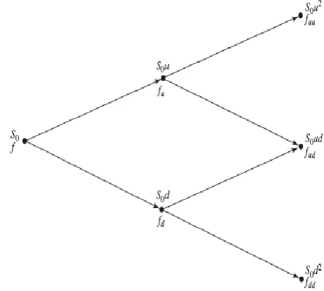
After one time period, the stock price can move up to
u
[image:3.595.318.549.555.762.2]S
0 with probabilityp
or down toS
0d
with probability(
1
p
)
as shown in the Fig. 1 below.Fig. 1: Stock and Option Prices in a General One-Step Tree Therefore the corresponding value of the call option at the first time movement
t
is given by [11]
)
0
,
max(
)
0
,
max(
0 0
K
d
S
f
K
u
S
f
d u
(14)
where
f
uandf
dare the values of the call option after upward and downward movements respectively.We need to derive a formula to calculate the fair price of the option. The risk neutral call option price at the present time is
)
)
1
(
(
u dt r
f
p
pf
e
f
(15)To extend the binomial model to two periods, let
uu
f
denote the call value at time2
t
for two consecutive upward stock movements,f
ud for one upward and one downward movement andf
ddfor two consecutive downward movement of the stock price as shown in the Fig. 2 below.Fig. 2: Binomial Tree for the respective Asset and Call Price in a Two-Period Model
IAENG International Journal of Applied Mathematics, 44:1, IJAM_44_1_05
Then we have
)
0
,
max(
)
0
,
max(
)
0
,
max(
0 0 0K
dd
S
f
K
ud
S
f
K
uu
S
f
dd ud uu (16)The values of the call options at time
t
are
)
)
1
(
(
)
)
1
(
(
dd ud t r d ud uu t r uf
p
pf
e
f
f
p
pf
e
f
(17) Substituting (17) into (15), we have:))
)
1
(
(
)
1
(
)
)
1
(
(
(
dd ud t r ud uu t r t rf
p
pf
e
p
f
p
pf
pe
e
f
)
)
1
(
)
1
(
2
(
2 22 dd ud uu t r
f
p
f
p
p
f
p
e
f
(18)(18) is called the current call value using time
2
t
, where the numbersp
2,2
p
(
1
p
)
and(
1
p
)
2 are the risk neutral probabilities that the underlying asset pricesSuu
,ud
S
0 andS
0dd
respectively are attained.We generate the result in (18) to value an option at
N
T
t
as j N jd u j N j N j t rNf
p
p
j
N
e
f
(
1
)
0
)
0
,
max(
)
1
(
0 0K
d
u
S
p
p
j
N
e
f
j N j j N jN
j t
rN
(19) where)
0
,
max(
S
0u
d
K
f
ujdN j
j N j
and!
)!
(
!
j
j
N
N
j
N
is the binomial coefficient. We assume that
m
is the smallest integer for which the option's intrinsic value in (19) is greater than zero. This implies thatSu
md
Nm
K
. Then (19) can be expressed asj N j N m j t rN j N j j N j N m j t rN
p
p
j
N
Ke
d
u
p
p
j
N
e
S
f
)
1
(
)
1
(
0 (20)(20) gives us the present value of the call option.
The term
e
rNt is the discounting factor that reducesf
to its present value. The first term ofj N j
p
p
j
N
)
1
(
is the binomial probability ofj
upwardmovements to occur after the first
N
trading periods andj N j
d
Su
is the corresponding value of the asset afterj
upward move of the stock price.The second term is the present value of the option`s strike price. Putting
R
e
rt, in the first term in (20), we obtainj N j N m j t rN j N j j N j N m j N
p
p
j
N
Ke
d
u
p
p
j
N
R
S
f
)
1
(
)
1
(
0 Therefore, j N j N m j t rN j N j N m jp
p
j
N
Ke
d
p
R
pu
R
j
N
S
f
)
1
(
)
)
1
(
(
)
(
1 10
(21)
Now, let
(
m
;
N
,
p
)
denotes the binomial distribution function given by
N m j j N j j Np
p
C
p
N
m
;
,
)
(
1
)
(
(22)
(22) is the probability of at least
m
success inN
independent trials, each resulting in a success with probabilityp
and in a failure with probability(
1
p
)
. Then letp
R
1pu
and(
1
p
)
R
1(
1
p
)
d
. Consequently, it follows from (21) that)
,
;
(
)
,
;
(
0
m
N
p
Ke
m
N
p
S
f
rt
(23)The model in (23) was developed by Cox-Ross-Rubinstein [4] and we will refer to it as CRR model for the valuation of European call option. The corresponding value of the European put option can be obtained using call-put parity of the form
C
E
Ke
rt
P
E
S
0. We state a lemma for CRR binomial model for the valuation of European call option.Lemma 1[7]: The probability of a least
m
success inN
independent trials, each resulting in a success with probabilityp
and in a failure with probabilityq
is given by
N m j j N j jN
C
p
p
p
N
m
;
,
)
(
1
)
(
Let
p
R
1pu
andq
R
1(
1
p
)
d
, then it follows thatf
S
0
(
m
;
N
,
p
)
Ke
rt
(
m
;
N
,
p
)
B. Procedures for the Implementation of the Multi-Period Binomial Model
When stock price movements are governed by a multi-step binomial tree, we can treat each binomial multi-step separately. The multi-step binomial tree can be used for the American and European style options.
Like the Black-Scholes model, the CRR formula in (23) can only be used in the pricing of European style options and is easily implementable in Matlab. To overcome this problem, we use a different multi-period binomial model for the American style options on both the dividend and non-dividend paying stocks. The no-arbitrage arguments are used and no assumptions are required about the probabilities of the up and down movements in the stock price at each node.
IAENG International Journal of Applied Mathematics, 44:1, IJAM_44_1_05
For the multi period binomial model, the stock price $S$ is known at time zero. At time
t
, there are two possible stock pricesS
0u
andS
0d
respectively. At time2
t
, thereare three possible stock prices
S
0uu
,S
0ud
andS
0dd
andso on. In general, at time
i
t
where0
i
N
,)
1
(
i
stock price are considered, given byN
j
for
d
u
S
0 j N j,
0
,
1
,
2
,...,
(24) where
N
is the total number of movements andj
is the total number of up movements. The multi-period binomial model can reflect numerous stock price outcomes if there are numerous periods. The binomial option pricing model is based on recombining trees, otherwise the computational burden quickly become overwhelming as the number of moves in the tree increases.Options are evaluated by starting at the end of the tree at time
T
and working backward. We know the worth of a call and put at timeT
is
)
0
,
max(
)
0
,
max(
T T
S
K
K
S
(25) respectively. Because we are assuming the risk neutral world, the value at each node at time
(
T
t
)
can be calculated as the expected value at timeT
discounted at rater
for a time period
t
. Similarly, the value at each node at time(
2
T
t
)
can be calculated as the expected value at time(
T
t
)
discounted for a time period
t
at rater
, and so on. By working back through all the nodes, we obtain the value of the option at time zero.Suppose that the life of a European option on a non-dividend paying stock is divided into
N
subintervals of length
t
. Denote thej
th node at timei
t
as the)
(
i
j
node, where0
i
N
and0
j
i
. Definej i
f
, as the value of the option at the(
i
,
j
)
node. The stockprice at the
(
i
,
j
)
node isSu
jd
Nj. Then, the respective European call and put can be expressed as)
0
,
max(
,
Su
d
K
f
N j
j Nj
(26),...
2
,
1
,
0
),
0
,
max(
,
j
for
d
Su
K
f
N j j N j (27)There is a probability
p
of moving from the(
i
,
j
)
node at timei
t
to the(
i
1
,
j
1
)
node at time(
i
,
j
)
t
and a probability((
1
p
)
of moving from the(
i
,
j
)
node at thet
i
to the(
i
1
,
j
)
node at time(
i
1
)
t
. Then the neutral valuation is
i
j
N
i
f
p
pf
e
f
ij rt i j i j0
,
1
0
]
)
1
(
[
1 ,1 1 ,,
(28) For an American option, we check at each node to see whether early exercise is preferable to holding the option for a further time period
t
. When early exercise is taken into account, this value off
i,j must be compared with theoption's intrinsic value [7]. For the American put option, we have that
, ,
,
,i j i j i j
f
P
f
0,
[
1 ,1(
1
)
1 ,]
, i j ij
t r j i j j
i
K
S
u
d
e
pf
p
f
f
(29)(29) gives two possibilities:
If
P
i,j
f
i,j, then early exercise is advisable. If
P
i,j
f
i,j, then early exercise is not advisable.C. Variations of Binomial Models
The variations of binomial models is of two forms namely underlying stock paying a dividend or known dividend yield and underlying stock with continuous dividend yield.
1) Underlying stock paying a dividend or known dividend yield
The value of a share reflects the value of the company. After a dividend is paid, the value of the company is reduced so the value of the share.
1
,...,
2
,
1
,
0
,
,...,
2
,
1
,
0
,
0
i
N
N
j
for
d
u
S
j N j(30)
1
,
,
,...,
2
,
1
,
0
,
)
1
(
0
i
i
N
N
j
for
d
u
S
j N j(31)
2) Underlying stock with continuous dividend yield A stock index is composed of several hundred different shares. Each share gives dividend away a different time so the stock index can be assumed to provide a dividend continuously.
We explored Merton's model, the adjustment for the Black-Scholes model to carter for European options on stocks that pays dividend. Here the risk-free interest rate is modified from
r
to(
r
)
where
is the continuous dividend yield. We apply the same principle in our binomial model for the valuation of the options. The risk neutral probability in (5) is modified but the other parameters remains the same.
e
d
e
u
d
u
d
e
p
t r
,
,
) (
(32)
These parameters apply when generating the binomial tree of stock prices for both the American and European options on stocks paying a continuous dividend and the tree will be identical in both cases. The probability of a stock price increase varies inversely with the level of the continuous dividend rate
.III. BLACK–SCHOLESEQUATION
Black and Scholes derived the famous Black-Scholes partial differential equation that must be satisfied by the
IAENG International Journal of Applied Mathematics, 44:1, IJAM_44_1_05
price of any derivative dependent on a non-dividend paying stock. The Black-Scholes model can be extended to deal with European call and put options on dividend-paying stocks, this will be shown later. In the sequel, we shall present the derivation of Black-Scholes model using a no-arbitrage approach.
A. Black-Scholes Partial Differential Equation
We consider the equation of a stock price
t t t
t
S
dt
S
dW
dS
(33) where
is the rate of return,
is the volatility and)
(
t
W
follows a Wiener process on a filtered probability space(
,
B
t,
,
F
(
B
t))
in which filtration)
0
,
{
)
(
B
B
t
F
t t , whereB
tis the sigma-algebra generated by{
S
t:
0
t
T
}.
Now, suppose that)
,
(
)
,
(
t
S
f
t
S
f
t
is the fair price of a call option or otherderivative contingent claim of the underlying asset price
S
at timet
. Assuming thatf
C
2,1(
R
,
[
0
,
T
])
then by the Ito’s lemma given below;
t s t s s tdW
x
U
d
x
U
U
W
s
U
W
t
U
2 2)
,
(
)
,
(
(34)We obtained the Black-Scholes partial differential equation of the form
0
2
2 2 2 2
rf
S
f
S
S
f
rS
t
f
(35) Solving the partial differential equation above gives an analytical formula for pricing the European style options. These options can only be exercised at the expiration date. The American style options are exercised anytime up to the maturity date. Thus, the analytical formula we will derive is not appropriate for pricing them due to this early exercise privilege [8].In the case of a European call option, when
t
T
, the key boundary condition is)
0
,
max(
S
K
f
(36) In the case of a European put option, whent
T
, the key boundary condition is)
0
,
max(
K
S
f
(37)B. Solution of the Black-Scholes Equation
We shall apply the boundary conditions for the European call option to solve the Black-Scholes partial differential equation. The payoff condition is
)
0
,
max(
)
,
(
t
T
S
S
K
f
(38)The lower and upper boundary conditions are given by
t E A t T r t E AS
K
t
S
C
K
t
S
C
Ke
S
K
t
S
C
K
t
S
C
)
,
,
(
),
,
,
(
)
,
,
(
),
,
,
(
( )These are the conditions that must be satisfied by the partial differential equation.
Let
T
t
, whereT
is the expiration date andt
is the present time. Since
T
t
f
t
f
f
t
f
t
t
f
t
f
1
1
(39)Substituting (39) into (35), yields
rf
S
f
S
S
f
rS
f
2 2 2 22
(40)Taking
y
ln
S
, then
2 2 2 2 2 21
1
1
1
y
f
S
y
f
S
y
f
S
S
S
f
S
S
f
y
f
S
S
y
y
f
S
f
Therefore,
2 2 2 2 2 21
1
1
y
f
S
y
f
S
S
f
y
f
S
S
f
(41)We now introduce a new solution
)
,
(
)
,
(
y
e
f
y
w
r, and then we have that
2 2 2 2)
,
(
y
f
e
y
f
y
f
e
y
f
y
w
re
w
e
f
r r r r
(42)Substituting (41) into (40), we have
rf
y
f
y
f
r
f
2 2 2 22
2
(43)Also substituting (42) into (43), yields
IAENG International Journal of Applied Mathematics, 44:1, IJAM_44_1_05
)
,
(
2
2
)
,
(
)
,
(
2
2
)
,
(
2 2 2 2 2 2 2 2
y
rw
y
w
y
w
r
y
rw
w
y
rw
y
w
y
w
r
y
rw
w
e
r
Therefore, 2 2 2 22
2
y
w
y
w
r
w
(44)(44) is called a diffusion equation which has a fundamental solution as a normal function.
2 2 22
2
exp
2
1
)
,
(
r
y
y
(45)So,
2 2 22
2
exp
2
1
)
,
(
r
y
y
(46)Since
y
ln
S
, theny
e
S
(47) The payoff for call option becomes)
0
,
max(
)
,
0
(
)
,
0
(
)
0
,
max(
)
0
,
max(
)
0
,
max(
)
,
(
K
e
w
f
K
e
K
e
K
S
S
t
f
)
0
,
max(
)
,
0
(
e
K
w
(48) The solution to (44) is
w
y
d
y
w
(
,
)
(
0
,
)
(
,
)
(49) We use the payoff condition in (48) and the fundamental solution of (46) to obtain
2 2 2 ln2
2
exp
)
max(
2
1
)
,
(
r
y
d
K
e
y
w
K (50)We denote the distribution function for a normal variable by
N
(
x
)
du
e
x
N
x u
2 22
1
)
(
(51)Then (51) becomes
2 2 2 ln ln2
2
exp
2
exp
2
1
)
,
(
r
y
d
e
K
d
e
y
w
K K (52) Let
2 2 2 22
2
ln
2
A
r
S
r
y
A
So (52) becomes
K Kd
A
e
K
d
A
e
y
w
ln 2 2 ln 2 22
)
(
exp
2
2
)
(
exp
2
1
)
,
(
(53)We consider the second term in the right-hand side of (53), that is
Kd
A
e
K
ln 2 22
)
(
exp
2
Setting
)
(
A
z
(54) Thendz
d
d
dz
1
and the limits of (53) using (54) are given below
K
when
r
K
S
r
S
K
A
K
z
when
z
ln
,
2
ln
2
ln
ln
ln
,
,
2 2
IAENG International Journal of Applied Mathematics, 44:1, IJAM_44_1_05
2
ln
2 2r
K
S
d
(55)Changing the variable from
toz
, the second term in the right-hand side of (54) becomes)
(
2
2
2 2 2 2 2 2 2 2d
KN
dz
e
K
dz
e
K
d zd z
(56)The first integrand of the first term in (53) is expressed as
2 2 2 2 2 22
)
(
2
exp
2
)
(
exp
A
A
A
e
2 2 2 2 2 2 2 22
)
(
)
(
)
(
2
exp
A
A
A
A
2 2 2 22
))
(
(
exp
2A
e
A (57)We use the definition of
A
to have r r y r y r y A
Se
e
e
e
e
e
2 2
2 2 2 2 Therefore, r A
Se
e
2
2
Then (57) becomes
2 2 2 2 22
))
(
(
exp
2
)
(
exp
A
Se
A
e
r(58) Substituting (58) into the first term of (53), we have
K rd
A
Se
ln 2 2 22
))
(
(
exp
2
1
By changing the variables as we did in the previous case, we get
z d r z rd
N
Se
dz
e
Se
(
)
2
1
1 2 2
(59)Where
z d zdz
e
d
N
2 1 22
1
)
(
and
2
ln
2 1r
K
S
d
(60)Whence (53) becomes
2
ln
2
ln
)
,
(
2 2r
K
S
KN
r
K
S
SN
e
y
w
r (61)Recall that
e
rw
(
y
,
)
f
(
y
,
)
C
E, hence)
(
)
(
d
1Ke
N
d
2SN
C
E r
(62)This is the Black-Scholes formula for the price at time zero of a European call option on a non-dividend paying stock [1]. We can derive the corresponding European put option formula for a non-dividend paying stock by using the call-put parity given by
P
E
C
E
S
Ke
r.The European put analytical formula is
)
(
)
(
d
2SN
d
1N
Ke
P
E
r
(63) whereN
(
d
1)
1
N
(
d
1),
N
(
d
2)
1
N
(
d
2)
The European call and put analytic formulae have gained popularity in the world of finance due to the ease with which one can use the formula for options valuation, the other parameters apart from the volatility can easily be observed from the market. Thus it becomes necessary to find appropriate methods of estimating the volatility.
C. Dividend Paying Stock
We relax the assumption that no dividend are paid during the life of the option and examine the effect of dividend on the value of European options by modified the Black-Scholes partial differential equation to carter for these dividends payments.
Now we shall consider the continuous dividend yield model, let
denote the constant continuous dividend yield which is known. This means that the holder receives a dividend
dt
with the time intervaldt
. The share value is lowered after the payout of the dividend and so the expected rate of return
of a share becomes(
)
. The geometric Brownian motion model in (33) becomest t t
t
S
dt
S
dW
dS
(
)
(64) and the modified Black-Scholes partial differential equation in (35) is given by0
2
)
(
2 2 2 2
rc
S
c
S
S
c
S
r
t
c
(65) Let
T
t
, solving (65) by applying the same method, the European call option for a dividend paying stock is given by)
(
)
(
d
1Ke
N
d
2N
Se
C
E
r
(66) and the European put option isIAENG International Journal of Applied Mathematics, 44:1, IJAM_44_1_05
)
(
)
(
d
2SNe
d
1N
Ke
P
E
r
(67) where
1 2 2 2 12
ln
,
2
ln
d
r
K
S
d
r
K
S
d
(68)The results in (66) and (67) can similarly be achieved by considering the non-dividend paying stock formulae in (62) and (63). The dividend payment lowers the stock price from
S
toSe
and the risk-free interest rate which is the rate of return fromr
to(
r
)
[7].D. Boundary Condition for Black-Scholes Model
The boundary conditions for Black-Scholes model for pricing a standard option are given by
)
0
,
max(
)
,
(
)
,
(
lim
,
0
)
,
0
(
K
S
t
S
f
S
t
S
f
t
t
f
c c S c (69)We shall state below some theorems without proof as follows:
Theorem 2 [7]: Under the binomial tree model for stock pricing, the price of a European style option with expiration date
t
T
is given byT T
r
f
E
f
)
1
(
)
(
* 0
(70)Corollary 3 [7]: Under the binomial tree model for stock pricing, the price of a European style option with expiration date
t
T
is given byT T j j T j j T j j T T T T T
r
K
d
u
S
p
p
C
r
K
S
E
r
f
E
f
)
1
(
)
0
,
(
)
1
(
)
(
)
1
(
))
0
,
(max(
)
1
(
)
(
0 0 * * * * 0
(71)where
E
* denotes expected value under the risk neutral probabilityp
*for stock price.The above Theorem 2 can be written in words as “the price of the option is equal to the present value of the expected payoff of the option under the risk neutral measure”.
Theorem 4: (Continuous Black Scholes Formula) [7]
Assume that
u
d
u
t
N
T
,
1
,
1
and define
0
such thatu
e
tandd
e
t. Then there holds
dy
e
x
N
d
N
Ke
d
SN
t
S
f
x y rT c t 2 2 1 0 22
1
)
(
)
(
)
(
)
,
(
lim
(72)where
N
(.)
is the cumulative function of the standard normal distributions.
T
d
T
T
r
K
S
d
T
T
r
K
S
d
1 2 2 2 12
ln
,
2
ln
(73)Theorem 5: Let
n,CRRbe then
period CRR binomial delta of a standard European put option with extended tree and
BSis the true delta. Therefore
n
O
n
f
n
e
d BS CRR n1
))
(
(
2
2 , 2 1
(74)where
1 2 1 2 2ln
ln
)
(
,
2
ln
)),
(
)
(
(
2
))
(
(
d
u
S
K
n
T
r
K
S
d
n
n
d
n
f
y
(75)and
m
is the largest integer which satisfiesK
d
Su
m nm
.IV. NUMERICALEXAMPLESANDRESULTS This section presents some numerical examples and results generated as follows;
A. Numerical examples
Example 1: Consider a standard option that expires in three months with an exercise price of
$
65
. Assume that the underlying stock pays no dividend, trades at$
60
, and has a volatility of30
%
per annum. The risk-free rate is8
%
per annum.We compute the values of both European and American style options using Binomial model against Black-Scholes model as we increase the number of steps with the following parameters:
IAENG International Journal of Applied Mathematics, 44:1, IJAM_44_1_05
30
.
0
,
08
.
0
,
25
.
0
,
65
,
60
K
T
r
S
The Black-Scholes price for call and put options are
1334
.
2
and5
.
8463
respectively.The results obtained are shown in Table I below.
Example 2: Binomial pricing results in a call price of
87
.
31
$
and a put price of$
5
.
03
. The interest rate is5
%
, the underlying price of the asset is$
100
and the exercise price of the call and the put is$
85
. The expiration date is in three years. What actions can an arbitrageur take to make a riskless profit if the call is actually selling for$
35
?Solution:
Since the call is overvalued and arbitrageur will not want to write the call, buy the put, buy the stock and borrow the present value of the exercise price, resulting in the following cash flow today as shown below
Write 1 call
$
35
Buy 1 put
$
5
.
03
Buy 1 share
$
100
Borrow$
85
e
0.053$
73
.
16
13
.
3
$
The value of the portfolio in three years will be worthless, regardless of the path the stock takes over the three-year period.
Example 3: Consider pricing a standard option on a stock paying a known dividend yield,
0
.
05
with the following parameters:17
.
0
,
25
.
0
,
1
.
0
,
25
.
0
,
50
T
r
S
The results obtained are shown in Table II below.
Example 4: We consider the performance of Binomial model against the “true” Black-Scholes price for American and European options with
25
.
0
,
1
.
0
,
5
.
0
,
40
,
45
K
T
r
S
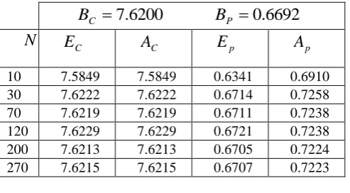
The results obtained are shown in the Table III below. The convergence of the binomial model to the Black-Scholes value of the option is also made more intuitive by the graph in Fig. 3 below.
Fig. 3: Convergence of the European Call Price for a Non-Dividend Paying Stock Using Binomial Model to the Black-Scholes Value Of
7
.
62
B. Table of Results
We present the results generated in the Tables I, II and III below.
TABLE I: THE COMPARATIVE RESULTS
ANALYSIS OF THE BINOMIAL MODEL AND BLACK SCHOLES VALUE
(
B
C
2
.
1334
,
B
P
5
.
8463
)
OF THE STANDARD OPTIONN
European Call,E
CAmerican Call,
A
CEuropean Put,
E
p